Muscle Fatigue in Musculoskeletal Numerical Models
Dissertation
zur Erlangung des Doktorgrades der Humanwissenschaften
(Dr. sc. hum.)
der
Fakult¨at f¨ur Medizin der Universit¨at Regensburg
vorgelegt von Simon J. Groß
aus Straubing
im Jahr 2018
Muscle Fatigue in Musculoskeletal Numerical Models
Dissertation
zur Erlangung des Doktorgrades der Humanwissenschaften
(Dr. sc. hum.)
der
Fakult¨at f¨ur Medizin der Universit¨at Regensburg
vorgelegt von Simon J. Groß
aus Straubing
im Jahr 2018
Dekan: Prof. Dr. Dr. Torsten E. Reichert
Betreuer: Prof. Dr.-Ing Sebastian Dendorfer
Tag der m¨undlichen Pr¨ufung:
Abstract
The investigation of the musculoskeletal system is a challenging task, since compre- hensive knowledge of muscle and joint forces within the human body is required.
Therefore, in recent years numerical models have been developed for a better understanding of the musculoskeletal system. Especially for the investigation of long-term effects, the issue of muscle fatigue needs to be taken into consideration in these models.
The objectives of this thesis was to develop a novel EMG based muscle fatigue al- gorithm and the implementation into a state-of-the-art musculoskeletal modelling system. This included the investigation of the progress of muscle fatigue of single muscles, as well as the behaviour of muscle recruitment pattern when experiencing fatigue.
Therefore, two experimental studies were conducted in the course of this thesis, in order to analyse the progress of muscle fatigue of single muscles in correlation with relative muscle loadings and to study the behaviour of muscle recruitment pattern of thorax muscles when experiencing fatigue. Based on the results of the first study a fatigue algorithm was developed and implemented to the AnyBody Modeling SystemTM (AMS). Both experimental studies were simulated in the al- tered AMS to validate the fatigue algorithm and to analyse the behaviour of the muscle recruitment solver of the modified system.
The results show a good correlation between the simulated muscle fatigue and the experimental data. Furthermore, it revealed a reduction of maximum force capacity of the muscles of about 10-15 % compared to the non-fatigued condition.
The analysis of the muscle recruitment pattern indicated an additional activation of muscles in the upper back as well as the abdomen. The numerical simulation of these exercises in the AMS revealed a shift of muscle activity to the upper back.
Kurzfassung
Die Untersuchung des muskuloskeletalen Apparates ist eine große Herausforderung, da hierzu m¨oglichst genaue Kenntnisse von Muskel- und Gelenkkr¨aften ben¨otigt werden. Daher wurden in den letzten Jahren numerische Modelle entwickelt, um einen genaueren Einblick in das muskuloskeletale System zu erhalten. Insbeson- dere um eine Aussage ¨uber Langzeiteffekte machen zu k¨onnen, muss die Erm¨udung von Muskeln ber¨ucksichtigt werden.
Ziel dieser Arbeit war die Entwicklung eines neuartigen Erm¨udungsalgorithmus basierend auf EMG Messungen. Dies beinhaltete die Untersuchung des Verlaufs der Erm¨uding einzelner Muskeln, sowie deren Einflusses auf Rekrutierungsmuster.
Des Weiteren wurde dieser Algorithmus in ein modernes muskuloskeletales Berech- nungssystem implementiert.
Im Zuge dieser Arbeit wurden zwei experimentelle Studien durchgef¨uhrt, um den Verlauf von Muskelerm¨udung einzelner Muskeln in Korrelation mit deren relativen Belastung zu ermitteln, sowie das Verhalten von Muskelrekrutierungsmustern der Thoraxmuskulatur w¨ahrend erm¨udender ¨Ubungen zu untersuchen. Basierend auf den Ergebnissen der ersten Studie wurde ein Erm¨udungsalgorithmus entwickelt und in das AnyBody Modeling SystemTM (AMS) implementiert. Beide experi- mentellen Studien wurden mit dem modifizierten AMS simuliert um den Algorith- mus zu validieren und das Verhalten des Rekrutierungssolvers zu untersuchen.
Die Ergebnisse der simulierten Muskelerm¨udung korrelierten gut mit den Daten aus der experimentellen Studie. Außerdem ergab sich eine Reduktion der maxi- malen Muskelkraft der belasteten Muskulatur um 10-15 % durch die Erm¨udung.
Die Analyse der Rekrutierungsmuster ergab eine zus¨atzliche Aktivierung entweder der oberen R¨uckenmuskulatur oder der Bauchmuskulatur bei den meisten Proban- den. Die numerischen Simulationen der ¨Ubungen im modifizierten AMS ergab eine Verschiebung der Muskelaktivit¨at hin zu der oberen R¨uckenmuskulatur.
Contents
1. Introduction 9
1.1. Objectives of the Thesis . . . 10
1.1.1. Experimental Quantification of Muscle Fatigue . . . 10
1.1.2. Experimental Study of Muscle Recruitment Pattern Under the Influence of Fatigue . . . 11
1.1.3. Development of a Novel Fatigue Algorithm and Implemen- tation to the AMS . . . 11
1.1.4. Validation of the AMS Muscle Recruitment with Included Muscle Fatigue . . . 11
1.2. Outline of This Thesis . . . 12
1.3. AnyBody Modeling SystemTM . . . 12
1.3.1. AnyBodyTM Managed Model Repository . . . 13
1.3.2. Scaling . . . 17
1.3.3. Muscle Recruitment . . . 19
1.3.4. Muscle Models . . . 21
1.4. Muscle Physiology . . . 22
1.4.1. Structure of Human Skeletal Muscles . . . 23
1.4.2. Process of Muscle Activation and Force Generation in Hu- man Skeletal Muscles . . . 25
1.4.3. Muscle Fatigue Mechanisms . . . 28
1.4.4. Measurement of Muscle Fatigue . . . 30
1.5. Electromyography (EMG) . . . 31
1.5.1. Signal Emergence . . . 31
1.5.2. Influencing Factors on the EMG Signal . . . 33
1.5.3. Surface EMG Measurement . . . 35
1.5.4. Surface EMG - Force Relationship . . . 38
5
Contents 6
1.5.5. EMG Signal Normalization . . . 40
1.5.6. Manifestation of Muscle Fatigue in the EMG signal . . . 46
2. Material and Methods 49 2.1. Investigation of Fatigue Progress of m. Biceps Brachii and m. Tri- ceps Brachii . . . 50
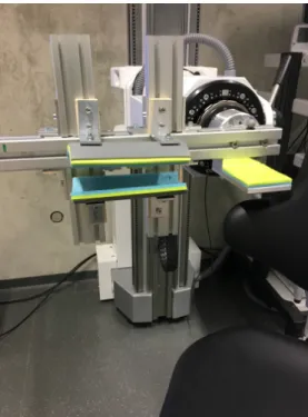
2.1.1. Experimental Set-up . . . 50
2.1.2. Summary Investigation of Fatigue Progress . . . 60
2.2. Development of Fatigue Algorithm, Implementation to AMS and Validation . . . 60
2.2.1. Fatigue Algorithm . . . 63
2.2.2. Recovery Model . . . 64
2.2.3. Endurance Time Model . . . 65
2.2.4. AnyBody ModelTM Set-up . . . 65
2.2.5. Summary Modified AMS Model of Upper Extremities . . . . 67
2.3. Experimental Study to Investigate Muscle Recruitment Pattern of the Back Muscles . . . 67
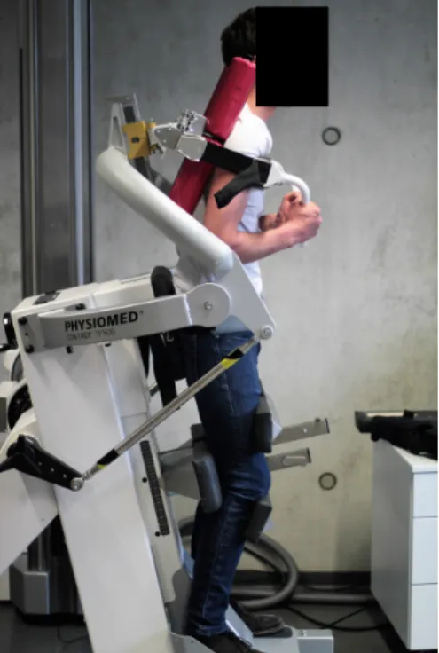
2.3.1. Experimental Set-up . . . 68
2.3.2. Subject Description . . . 69
2.3.3. Study Protocol . . . 69
2.3.4. Anthropometric Data . . . 71
2.3.5. Reference Values for Normalization and Relative Muscle Load- ing . . . 72
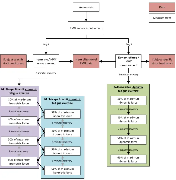
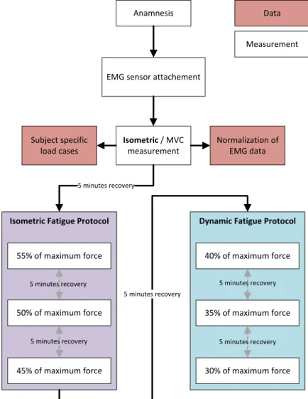
2.3.6. Isometric Fatigue Protocol . . . 73
2.3.7. Dynamic Fatigue Protocol . . . 73
2.3.8. Data Processing . . . 73
2.3.9. Summary Experimental Study Muscle Recruitment Pattern . 76 2.4. Investigation of AMS Recruitment Algorithm with Implemented Fa- tigue . . . 76
2.4.1. AnyBodyTMModel to Investigate Muscle Recruitment Pattern 77 2.4.2. Summary Recruitment Pattern of modified AMS Model . . . 80
Contents 7
3. Results 81
3.1. Experimental Study of Muscle Fatigue Progress . . . 81
3.1.1. Results from Isometric Fatigue Protocol . . . 82
3.1.2. Results from Dynamic Fatigue Protocol . . . 88
3.2. Results of the Developed Novel Fatigue Algorithm and Its Validation 90 3.2.1. Model Parameters for the AMS Model and the Implemented Fatigue Algorithm . . . 90
3.2.2. Validation of the Fatigue Algorithm in the AMS Model . . . 91
3.3. Experimental Study of Muscle Recruitment Pattern . . . 95
3.3.1. Results from Isometric Fatigue Protocol . . . 96
3.3.2. Results from Dynamic Fatigue Protocol . . . 98
3.4. Recruitment Pattern Modified AMS Model . . . 100
3.4.1. Model Parameters for the Simulation and Validation of the Muscle Recruitment Pattern . . . 101
3.4.2. Results from Simulated Muscle Recruitment . . . 101
4. Discussion 107 4.1. Fatigue Progress of Single Muscles . . . 108
4.2. Fatigue Algorithm and Implementation to AMS Model . . . 111
4.3. Muscle Recruitment Pattern - Experimental Study . . . 114
4.4. Muscle Recruitment Pattern - AMS . . . 117
5. Conclusion 119
A. Work Packages of the Thesis 142
B. Additional AnyBodyTM Source Code of Upper Limb Model 147 C. Segments and Muscles of the AMS Model to Simulate Fatigue of Shoulder
and Arm Muscles 151
D. Segments and Muscles of the AMS Model to Study Muscle Recruitment
Pattern 154
E. Additional Results of Experimental Study of Muscle Fatigue Progress 161
List of Acronyms and Symbols
Acronyms and symbols used in this thesis are listed subsequently.
Acronyms
AMS AnyBody Modeling SystemTM AAU Aalborg University
ADP Adenosine diphosphate
AMMR AnyBody managed model repository AP Action potential
ATP Adenosine triphosphate BMI Body mass index CNS Central nervous system CT Computed tomography DoF Degree of freedom ECG Electrocardiographic EMG Electromyographic
FDK Force-dependent kinematics FFT Fast Fourier transform MET Maximum endurance time MPF Median power frequency MSD(s) Musculoskeletal disorder(s) MU(s) Motor unit(s)
MUAP Motor unit action potential MVC Maximum voluntary contraction PCSA Physiological cross-sectional area RMS Root-mean-square
SD Standard deviation
SENIAM Surface EMG for a non-invasive assessment of muscles TELEM Twente lower extremity model
TKE Teager-Kaiser-Energy
8
1. Introduction
Analyses of the musculoskeletal system are challenging tasks since measurements of joint and muscle forces within the human body are not or hardly possible at all.
Therefore, in recent years numerical models have been developed to enhance the knowledge about the musculoskeletal system and to calculate the muscle and joint forces based on subject-specific data. The Anybody Modeling SystemTM (AMS) (AnyBody Technology A/S, Aalborg, Denmark) is a system for generating highly developed musculoskeletal models with a realistic level of complexity [1]. These models are validated and work well to analyse single motions or short motion cycles with relatively low intensity and allow the investigation of muscle and joint reaction forces. Therefore, these models are a useful tool when studying the musculoskeletal system and musculoskeletal disorders (MSDs). MSDs were the most common cause of work-related absence in 2016 [2] and often muscle fatigue is involved in these disorders [3]. In most cases, these MSDs are progressive disorders, as a result of muscles being loaded over a long period of time. The symptoms vary from discomfort followed by pain up to invalidity [4]. Therefore, a good understanding of the mechanics of the human body is required to be able to analyse long-term effects properly. However, when investigating long-term effects with numerical models, the issue of muscle fatigue needs to be taken into consideration, which is not yet represented in the AMS.
Different algorithm have been proposed in the last years to describe muscle fatigue.
When experiencing fatigue, the maximum force capacity of a muscle is reduced over time. The algorithm published by Ma et al., 2009b [5], for example, describes this. The model though is validated against the maximum endurance time of the exercises and thereby, total exhaustion is reached when the muscle can no longer produce the required force. This means that the model overestimates the reduction
9
1.1. OBJECTIVES OF THE THESIS 10 of maximum force capacity during fatigue, since the contribution of central fatigue and peripheral fatigue are not considered [6, 7]. Another example for a numerical fatigue model was published by Silva et al., 2011 [8], in which the central fatigue was also excluded from the study.
Electromyographic (EMG) measurements are the most common tool to investigate muscle fatigue. Furthermore, the myoelectric signal is influenced not only by the fatigue of the muscle itself, but by central fatigue and peripheral fatigue as well.
Therefore, the development of a fatigue algorithm based on EMG measurements is required for a realistic assessment of its influence on muscle force generation. To gain a closer insight into the musculoskeletal system when experiencing fatigue, it is necessary, to implement this novel fatigue algorithm to a state-of-the-art simulation tool.
1.1. Objectives of the Thesis
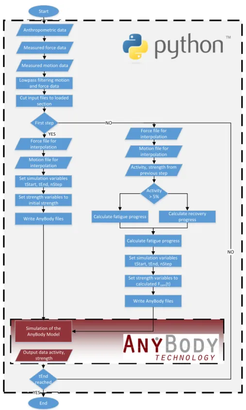
In this thesis, fundamental research regarding the simulation of the effect of mus- cle fatigue on the musculoskeletal system is presented. The workflow conducted throughout the study can be grouped into four different work packages which are described in the following. A detailed overview of the work packages is shown in tables A.1 - A.4.
1.1.1. Experimental Quantification of Muscle Fatigue
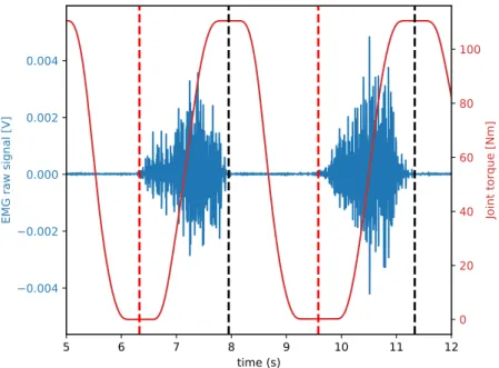
The first step was the quantification of muscle fatigue based on EMG measure- ments. The study was designed to investigate the progress of muscle fatigue of single muscles during isometric and dynamic contraction in relation to the relative muscle loading. This novel approach was required for the development of the fa- tigue algorithm, which was based on the results from this experimental study. The progress of muscle fatigue was estimated with the maximum voluntary contraction (MVC) normalized root mean square (RMS) of the EMG signal. Furthermore, the median power frequency (MPF) was analysed in order to verify the muscle fa- tigue during the recorded exercises. The recorded data was also used to validate the modified AMS model including the fatigue algorithm which was developed in
1.1. OBJECTIVES OF THE THESIS 11 work package three.
1.1.2. Experimental Study of Muscle Recruitment Pattern Under the Influence of Fatigue
The second work package aimed to investigate the influence of muscle fatigue on the recruitment pattern of muscles. Therefore, an experimental study was designed, where the EMG signals of 16 muscles of the back and abdomen were collected during exhausting isometric and dynamic exercises. This data was evaluated for potential changes in the global muscle recruitment of back and abdominal muscles when experiencing fatigue. The data was also used to validate the recruitment algorithm of the modified AMS model including the novel fatigue algorithm.
1.1.3. Development of a Novel Fatigue Algorithm and Implementation to the AMS
The aim of the third work package was the development of a novel fatigue algorithm based on the results from the first work package. Furthermore, the implementation to the AMS was also part of this work package, including the validation of the developed model against measured data. The designed algorithm allowed the estimation of the current maximum muscle force capacity of single muscles when experiencing fatigue and therefore provides an insight into the musculoskeletal system during long-term loadings.
1.1.4. Validation of the AMS Muscle Recruitment with Included Muscle Fatigue
The modified AMS model developed in the third work package was extended to simulate the exercises from the experimental muscle recruitment study. Addi- tionally, all exercises were simulated with the generic AMS model without any modifications to analyse the behaviour of the muscle recruitment algorithm of the AMS. The calculated muscle forces were investigated focusing on global muscle recruitment of back and abdominal muscles.
1.2. OUTLINE OF THIS THESIS 12
1.2. Outline of This Thesis
The thesis is structured in four major chapters. In the first chapter, basic in- formation about the AMS, muscle physiology, muscle fatigue in general and elec- tromyographic measurements is provided. The second chapter is complemented with information about the set-up of the conducted experimental studies, as well as the development of the fatigue algorithm. Furthermore, the structure of the modified AMS models for the validation of the fatigue and recruitment algorithm is described. In the third chapter, the results from the experimental studies and from the validation simulations are presented. These results are discussed in chap- ter 4, followed by a brief summary in chapter 5.
1.3. AnyBody Modeling System
TMAnyBody Technology A/S is a spin-off from the University of Aalborg, Denmark where the AMS was originally developed. In this chapter the AMS is described in detail with a special focus on the recruitment of muscles.
According to Damsgaard et al., 2006 [1] the AMS was developed as a tool to create musculoskeletal models from scratch or to modify existing models. It should also allow the exchange of models and the cooperation on model development. Another aim when designing the AMS was to allow ergonomic design optimization studies.
Furthermore, the system should be able to handle models with a level of detail as high as possible.
The models in the AMS are based on the methods of multi-body modelling systems.
Therefore, the generic model consists of rigid-bodies as bones connected by joints, ligaments and muscle-tendon units. Drivers for each joint restrict the degrees of freedom of each segment, allowing time depending kinematics. External loads and forces can also be applied in the AMS as time dependent boundary conditions. To calculate the variables like muscle force, joint reaction forces, etc. inverse dynamic routines are applied. Therefore, the motion of the body needs to be specified. In comparison to forward dynamic models, this method is much more efficient [1].
Since the development of a whole human body model is a very challenging and elaborating task, the AMS provides a model repository, the so called AnyBodyTM
1.3. ANYBODY MODELING SYSTEMTM 13 Managed Model Repository (AMMR). The AMMR consists of several different body models and application models like for example the ’HumanStanding’ model which is shown in figure 1.1. The models from the AMMR can be adjusted by the
Figure 1.1.: Full body human standing model from the AMMR (v.2.1.1) user so that the development of an entirely new model is not required.
The following chapters give a brief overview of the model set-up and mechanisms.
Furthermore, the validation of the models is described.
1.3.1. AnyBody
TMManaged Model Repository
The generic model for the AMMR was developed at Aalborg University (AAU) and is therefore called AAUHuman full body model. The information about this model is taken from the documentation of the AMMR v2.1.1 [9]. Since then, many different research facilities have developed different body parts for this model and increased the level of detail progressively. The most important models are presented in the following.
1.3. ANYBODY MODELING SYSTEMTM 14 Lumbar Spine
The lumbar spine model consists of five vertebrae which are connected by three DoF joints. The lumbar muscles are represented by a total of 188 muscle fascicles, which do not consider the force-length-velocity relation. Additionally, a model to calculate the intra-abdominal pressure is applied. In this model two assumptions were made. The first one is that only the transversus muscles contribute to the abdominal pressure. The second assumption is that the pressurized column is idealized as a cylinder. The abdominal model includes five artificial segments (disks) which are connected to one vertebra each (see figure 1.2). Furthermore, a reaction force between the buckle segment and each of these disks is modelled.
The transversus muscles are placed around these disks and are connected to the buckl segment. As the transversus muscles change length, the cross sectional area of the artificial disks, which are idealized as a circle change size. The force of the transversus muscles on the disks are balanced by the abdominal pressure which affects the reaction force on the lumbar spine. This allows the transversus muscles to function as an indirect spine extensor. The inter-vertebrae motions are considered by kinematic rhythms as a function of overall lumbar curvature. The facet joints are not represented in the model.
Disk 1 Disk 2
Disk 3 Disk 4
Disk 5
Buckl
Figure 1.2.: Abdominal model of the AMS
1.3. ANYBODY MODELING SYSTEMTM 15 Cervical Spine
The model of the cervical spine consists of seven vertebrae which are connected with three DoF joints, except for the joint between the C2 and the skull which only has one DoF. The muscles are represented by 136 muscle fascicles. The centre of rotation between vertebrae is modelled according to Amevo et al., 1991 [10].
Arm Model
The arm model was developed using data based on two cadaver studies. The joints and kinematic constrains of the arm model are shown in table 1.1.
Table 1.1.: Joints and kinematic constrains of the arm model [9]
Name Description Joint/Construction Type SC SternoClavicular Spherical Joint
AC AcromioClavicular Spherical Joint GH Glenohumeral Joint Spherical Joint
AI One DoF constraint requiring the bony
landmark AI on the scapula to stay in contact with the thorax
AA One DoF constraint requiring the bony
landmark AA on the scapula to stay in contact with the thorax
Conoideum- Ligament
The length of this ligament is driven to always remain constant
FE Flexion-extension of the elbow
Revolute Joint PS Pronation-supination
joint for the forearm
Combination of joints at the distal and proximal end of the radius bone that leaves one DoF free which is pronation/
supination of the forearm
Wrist Joint Two successive revolute joints where the axes of rotations are not coincident Leg Model
The basic leg model includes the pelvis, thigh, shank and the foot which is repre- sented by one segment. Furthermore, 35 muscles are defined. A spherical joint is used to model the hip joint, while the knee and ankle are specified as hinges.
1.3. ANYBODY MODELING SYSTEMTM 16 A more detailed leg model is the so calledTwente lower extremity model (TELEM) which is available in two versions.
The version 1.2 contains 159 muscles and has six joint degrees. It is based on a published anatomical dataset [11] and validated against literature with a focus on biomechanical performances.
The version 2.1 (TELEM2) includes 169 muscles. The model is based on a single consistent anatomical dataset which was derived at the University of Twente, The Netherlands [12]. In the new version, the surface wrapping of several muscles has been updated and the muscle attainment points and bone surfaces origin from a single subject which makes it more consistent.
Other Body Models
The body models also include two different mandible models. The symmetric mandible model is based on a CT scan of a 30-year-old male subject and contains 24 hill-type muscles and four DoF [13]. The second model is the so called Aalbor mandible. This model is based on the CT scan of a 40-year-old male subject. It features force-dependent kinematics (FDK) for the temporomandibular joint [14].
Thedetailed hand model is a model only designed for dynamic analysis, since there are no muscles included. The carpal bones are represented by 17 DoF.
Application Examples
The AMMR provides many different application examples. Starting from the
’StandingModel’ to ’CrossTrainer’ or ’BikeModel’ to ’AirlinePassenger’ model only to mention some examples, the user can choose which model fits closest to the motion of interest and modify this model. Furthermore, the AMMR includes different motion capture models. These models provide the opportunity to use C3D files from motion capture measurements as boundary conditions to drive the model which allows a very high kinematic accuracy. Models like the ’Spine Fixation Model’ are included mainly for studies in the area of orthopaedics and rehab.
A detailed list of all available models is available on https//anyscript.org[9].
1.3. ANYBODY MODELING SYSTEMTM 17
1.3.2. Scaling
Since the basic generic model represents the 50thpercentile European male human, scaling of the model is required to allow subject-specific modelling. A list of scaling laws that are available in the AMS is given in table 1.2.
Table 1.2.: Scaling laws available in the AMS [9]
Scaling law Description
ScalingStandard Scale to a standard size; i.e. use 50th percentile sizes for a European male
ScalingNone Do not scale; i.e. use underlying cadaveric dataset as it is
ScalingUniform Scale segments equally in all directions; input is joint to joint distances
ScalingLengthMass Scale taking mass into account; input is joint to joint distances and mass
ScalingLengthMassFat scale taking mass and fat into account; input is joint to joint distances
ScalingUniformExt Scale equally in all directions; input is external measurements
ScalingLengthMassExt Scale taking mass into account; input is external measurement
ScalingLengthMassFatExt Scale taking mass and fat into account; input is external measurements
ScalingXYZ Scale taking mass and fat into account; scale seg- ments along X, Y, Z axes; input is scale factors along X, Y, Z axes
Details about the scaling in the AMS are described by Rasmussen et al., 2005 [15].
The following information is taken from the aforementioned. The basic equation for linear scaling is defined as:
s =S·p+tr (1.1)
where s is the position of a local node on the scaled segment, p is the original position of the node, tr is the translation and S is the 3 x 3 scaling matrix defined
1.3. ANYBODY MODELING SYSTEMTM 18 as:
S=
S11 0 0 0 S22 0 0 0 S33
(1.2)
The scaling law mostly used in the AMS is the Length-Mass Scaling with fat percent. The parameters of the main diagonal of equation 1.2 are calculated as:
S22=kL = L1
L0 (1.3)
whereL1 is the new length of the scaled segment and L0 is the initial length. The ratio of masses of the segment is described by:
km = m1
m0 (1.4)
S11 and S33 are defined as:
S11=S33 =
skm
kL (1.5)
This formulation allows an inclusion of the fat percent for the scaling the strength of the model. The percent of muscle tissue is calculated by the equation:
Rmuscle = 1−Rf at−Rother (1.6)
withRother is the percent of skeleton, organs, blood, etc. The strength scale model is estimated by the function:
F =F0km kL
Rmuscle,1
Rmuscle,0 =F0km kL
1−Rother,1−Rf at,1
1−Rother,0−Rf at,0 (1.7) When no measurement of the fat percent is available, [16] proposed a method to calculate theRf at for women and men.
For women:
Rf at=−0.08 + 0.0203·BM I−0.000156·BM I2 (1.8)
1.3. ANYBODY MODELING SYSTEMTM 19 For men:
Rf at =−0.09 + 0.0149·BM I−0.00009·BM I2 (1.9)
1.3.3. Muscle Recruitment
The AMS allows the estimation of joint and muscle force in the human body.
The algorithms which need to be solved for this are described in the following chapter. The information presented is from the documentation of the AMS and the provided tutorials (Anybody Tutorials v7.1.2). Inverse dynamic is used in the AMS to calculate joint reactions and muscle forces in the AMS. Compared to the forward dynamic approach, this allows the analysis of large musculoskeletal systems with a relatively low computational effort. A simplified model of the forearm is shown in left figure 1.3.
Figure 1.3.: Simplified arm model (left); anatomical realistic model of human up- per extremity (right)
The known magnitude of the external load combined with the length of the forearm and the insertion point of the muscle allows the estimation of the muscle force by solving the momentum equilibrium about the elbow. The reaction force within the elbow joint can also be estimated by equilibrium equations.
When calculating a realistic musculoskeletal system as shown on the right side of figure 1.3 the complexity of equilibrium equations increases with each additional muscle. Further complications come with inertia terms which need to be considered during dynamic motion a well as the wrapping of muscles around bones and joints.
In addition, the human body has more muscles than required to balance all DoFs.
The AMS therefore provides different muscle recruitment algorithms which will be shown in the next paragraphs. Rasmussen et al., 2001 [17] describes how the
1.3. ANYBODY MODELING SYSTEMTM 20 muscle forces are calculated. A brief overview is given in this paragraph. The muscle recruitment in the AMS determines which set of muscle forces is used to balance a certain external load. The basic equilibrium equations can be written as:
Cf =r (1.10)
where C is the coefficient matrix, f contains the muscle and joint forces and r is the vector containing the external loads and inertia forces. This linear system of equations is usually easy to solve. However, due to muscles only producing force in one direction and the former mentioned muscle redundancy, there are more unknowns than equations in the system which leads to infinitely many possible solutions. Experimental studies have shown that the recruitment of muscles tend to be systematically. This consideration leads to the following optimization problem:
minimize G(f(M)) subject to Cf =r
fi(M) ≥0, i= 1...n(M)
(1.11)
G(f(M)) represents the body loads and n(M) is the number of muscles. The con- strains only apply to the muscles to ensure only forces in one direction. [17]
distinguishes two different objective functions. The polynomial criteria (1.12) is the most popular objective function.
G(f(M)) =
n(M)
X
i=1
fi(M) Ni
p
(1.12) Ni are normalization factors or functions like assumed maximum muscle strength, physiological cross-section area (PCSA), or the strength of the muscle at time instant. Polynomial objective functions require additional constraints to prevent single muscles to exceed their physiological maximum force with increasing external load.
The objective function includes a variable power p. This parameter controls how fast muscles are activated and deactivated. A value ofp= 1 leads to a recruitment of only the stronger muscles which is agreed to be non-physiological. Increasing
1.3. ANYBODY MODELING SYSTEMTM 21 the power leads to a more realistic reflection of the human muscle recruitment, hence to an increasing degree of synergism. Too high values forp result in a very quick, non-physiological activation and deactivation of muscles. Furthermore, high values of p can lead to numerical instabilities.
With increasing order of the objective function the solution converges with the so-called min/max objective function:
G(f(M)) =max
fi(N) Ni
, i= 1, ..., n(M) (1.13) This criterion results in a relative muscle force that is as small as possible. This means that the activation of all muscles contributing to balancing the external load is identical. This criterion has not only numerical advantages but is also physi- ological interesting, since maximum synergism leads to minimum fatigue of the muscles. Disadvantages of this criterion are that muscles are switched in and out very abruptly. Furthermore, muscles with only marginally positive contribution are also fully activated.
1.3.4. Muscle Models
In this chapter the different muscle models which are available in the AMS are described. The information is taken from the documentation AnyBody Tutori- als v.7.1.2.
Basically, there are two different approaches to describe muscle behaviour. The first approach is based on the work of Hill, 1938 [18]. In this model, the muscle is represented as a contractile element, combined with elastic elements. The model is proven to represent the behaviour of muscles quite well and has the advantage of being very efficient in numerical simulations.
The second approach is based on the work of Huxley, 1957 [19]. This model de- scribes the cross bridge activity during muscle contraction by differential equations and is therefore much more demanding to compute.
Classic numerical muscle model need to be adjusted to be used in inverse dynamic computation since usually these models need the activity of the muscle as input to calculate the muscle force. The AMS provides four different muscle models.
1.4. MUSCLE PHYSIOLOGY 22 AnyMuscleModel The simplest muscle model is the so-called AnyMuscleModel.
The only required input variable is the strength of the muscle at its optimal length.
Therefore, the contraction velocity or length of the muscle is not considered in this model. Although it is known that muscles do not behave this way, it provides good results for many cases. Different studies describe the correlation between the strength of the muscle and the cross-sectional area [20–23] which are reported for the major muscles from cadaver studies.
AnyMuscleModel3E The AnyMuscleModel3E in the AMS is Hill-model-based on the model published by Zajac, 1989 [24]. This model considers parallel passive elasticity of the muscle, serial elasticity of the tendon pennation angle of the fibres and other parameters. Furthermore, the model applies non-linear force-length and force-velocity relationship.
AnyMuscleModel2ELin The AnyMuscleModel2ELin is also a multi-element model.
The strength is proportional to the length of the muscle and the contraction ve- locity at time instant. The tendon is modelled as a linear-elastic element. The disadvantage of this model is that in some cases, if the muscle is stretched far enough, the active muscle force can be switched off entirely since the passive ele- ments always produce force while the muscle is elongated.
AnyMuscleModelUsr1 The AnyMuscleModelUsr1 provides the opportunity for the user to define a muscle model. The strength of the muscle can be defined as a function of different variables, including isometric strength, volume or PCSA, fibre length, kinematic measures and time.
1.4. Muscle Physiology
In this section, the basic physiology of human muscles is explained. Most infor- mation is taken from Schmitt, 1993 [25]. Basically three different types of muscles are distinguished in the human body:
• cardiac muscle
• smooth muscles
1.4. MUSCLE PHYSIOLOGY 23
• skeletal muscles
The cardiac muscle is a muscle type which is only found in the heart. Smooth muscles are found in the walls of hollow organs like the uterus, stomach, urinary bladders or in the walls of arteries, veins and the respiratory system. The function of the skeletal muscles is mainly the voluntary active motion of the human body.
Therefore, in the following the structure and processes of skeletal muscles are described in more detail.
Skeletal muscles represent about 40 % of the body weight. Overall more than 400 different muscles are distinguished. Each muscle is connected to at least one of each of the following parts:
• artery for oxygen and nutrient delivery
• vein for removal of metabolic waste products
• efferent nerves
• afferent nerves from muscle tendon spindles
• fibres from automatic nervous system
1.4.1. Structure of Human Skeletal Muscles
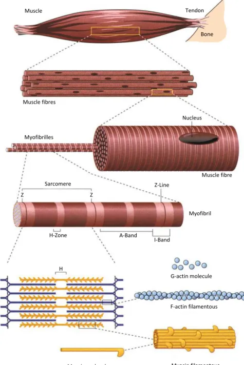
Each human muscle is constructed from muscle fibres with a diameter of approx- imately 50µm and a length of up to several centimetres. Skeletal muscles con- sist mostly of water (about 80 %). The main solid component are proteins, of which about 50 % are the contractile proteins myosin (35 %), actin (15 %) and tropomyosin-troponin (10 %). The contractile fibres are mainly constructed by myofibrils, from which each one is surrounded by the sarcoplasmatic reticulum.
Furthermore, mitochondria, glycogen granules and nuclei are embedded. The mi- tochondria are important for the generation of adenosine triphosphate (ATP), which is necessary in the process of the cross-bridge formation (see section 1.4.2).
Figure 1.4 shows the construction of a skeletal muscle.
1.4. MUSCLE PHYSIOLOGY 24
Bone
Muscle Tendon
Muscle fibres
Nucleus
Myofibrilles
Sarcomere
Muscle fibre Z-Line
H-Zone A-Band
I-Band
Myofibril Z
Z
H G-actin molecule
F-actin filamentous
Myosin molecule Myosin filamentous
Figure 1.4.: Construction of a human skeletal muscle (modified after Bloom &
Fawcett, 1986 [26])
1.4. MUSCLE PHYSIOLOGY 25
1.4.2. Process of Muscle Activation and Force Generation in Human Skeletal Muscles
The motor unit is the smallest functional unit to describe the neural control of muscle contraction and consists of the motor neuron with its dendrites and axon, together with the muscle fibres which are innervated by the axon [27]. The motor neuron receives its input from the central nervous system (CNS) and is located in the spinal cord or the brain stem. The axon connects the motor neuron and the muscle fibres, which it innervates [28]. All motor neurons that are connected to a muscle are known as a motor nucleus or motor neuron pool [29].
While in resting condition, the muscle fibre membrane has a potential of approx- imately -80 to -90 mV, which is maintained by the so-called ion pump [30]. The activation of a motor neuron results in the conduction of the excitation along the axon, which leads to the release of transmitter substances at the motor endplates.
The resulting endplate potential causes a slight modification of the diffusion char- acteristics of the muscle membrane and allows N a+ ions to flow into the muscle cell, which leads to a depolarisation of the transverse tubular system and sar- coplasmic reticulum. When exceeding a certain threshold, the action potential (AP) changes from about -80 mV to +30 mV and is reversed instantly. A hyperpo- larization phase is following the repolarisation phase during which the muscle fibre cannot be activated for a short time. The AP is schematically shown in figure 1.5 and is often referred to as the motor unit action potential (MUAP).
1.4. MUSCLE PHYSIOLOGY 26
Figure 1.5.: Action potential; Phase 1: Resting phase of AP, Phase 2: Depolar- ization, Phase 3: Rising phase of AP, Phase 4: Falling phase of AP, Phase 5: Undershoot (hyperpolarisation) [31]
The depolarization and repolarisation of the transverse tubular system and sar- coplasmic reticulum moves in a wave (electrical dipole) [32] across the muscle fibre bidirectionally starting from the endplates with a speed of about 2 - 6 m/s [30]
and causes a release of Ca2+ in the sarcoplasmic reticulum. The shortening of a sarcomere is initiated by the release of thisCa2+, which spreads over the contrac- tile filaments of actin and myosin. The binding of Ca2+ with tropin changes its shape by moving tropomyosin away from the binding sites of actin. This allows the myosin head to bind to actin and to form a cross-bridge. Adenosine diphos- phate (ADP) is released from the myosin head which causes its rotation and a force generation towards the middle of the sarcomere. When ATP binds to the myosin head, the cross-bridge is detached. The ATP is hydrolysed to ADP and organic phosphate which causes the myosin head to return to its initial position so that it can form another cross-bridge. The cross-bridge cycle repeats as long as the binding sites of actin are exposed. The muscles relaxes when intracellular calcium ([Ca2+]i) is actively returned to the sarcoplasmic reticulum which causes the recuperation of the blockade of the cross-bridge cycle and therefore a reduction of the produced force. The process of activation, contraction and relaxation can be described by 15 steps, where steps 1-6 describe the excitation, 7-10 the contraction
1.4. MUSCLE PHYSIOLOGY 27 and 11-15 the relaxation of the muscle:
1. Depolarization of end-plate membrane
2. Triggering of AP outside of end-plates and transmitting the AP across fibre surface
3. AP spreading into the fibre through tubular system
4. Release of Ca2+ from terminal cisterns of sarcoplasmatic reticulum, leading to an increase of [Ca2+]i and diffusion of Ca2+ to the contractile filaments 5. Binding of Ca2+ to troponin of thin filaments
6. Lifting of the blockade of cross-bridge cycle due to changes of the shape of troponin
7. Formation of cross-bridge
8. Force towards the middle of the sarcomere caused by rotation of myosin head 9. Binding of the ATP causes detachment of myosin head from actin and a
backwards rotation to the starting position 10. Hydrolysis of bound ATP
11. Absorption ofCa2+ by sarcoplasmic reticulum by decreasing [Ca2+]i
12. Releasing ofCas+ from troponin, back diffusion and absorption by sarcoplas- mic reticulum
13. Recuperation of blockade of cross-bridge cycle
14. Reduction of force by breaking cross-bridges without a new formation 15. Preparation of myosin heads for next contraction
1.4. MUSCLE PHYSIOLOGY 28
1.4.3. Muscle Fatigue Mechanisms
Muscle fatigue is studied for various applications such as rehabilitation medicine, sports, occupational medicine, space medicine, prostheses control or oncology [33].
Furthermore, it plays an important role in the fields of ergonomics. There are dif- ferent definitions of muscle fatigue. Edwards, 1981 [34] defined fatigue as failure to maintain required or expected force. Heimer states, that fatigue is a temporarily lowered capacity to perform work of a certain intensity caused by the work itself [35]. In general, fatigue is defined as any exercise-induced reduction in maximal capacity to generate force output [36]. According to Merletti et al. 2016, fatigue can be subdivided into fatigue of the CNS and the neuromuscular junction, or pe- ripheral fatigue, describing changes of muscle force generating capability [33]. The generation of muscle force is influenced by different factors, which are explained in the following.
Contribution of the neural system
Changes in the CNS or proximal to the neuromuscular junction are referred to as central fatigue. Neurotransmitters play an important role during this fatigue. For example Serotonin has been proven to have a negative influence on the performance during an exercise [37]. As described in section 1.4.2, the activation of motor units (MUs) is triggered by an input from the CNS on the spinal motoneurons by neurotransmitters. The strength output and timing of the contraction of the muscle fibre is controlled by the firing rate of the MU which is approximately 50 Hz - 60 Hz in healthy humans during a non-fatigued contraction [38]. Since the firing rate of the MUs is directly related to the force output of the muscle, a slowing or cessation of the MUs firing contributes to muscle fatigue. The firing rate is influenced by intrinsic in motoneuron properties and influenced by different factors [39]. It was found by Taylor et al. 2016, that repetitive activation of motoneurons lead to a reduced excitability [40]. The excitatory drive from the motor cortex or the supraspinal areas to the motoneurons is also negatively affected by intensive exercise and therefore lower, which leads to reduced firing rate of MUs [40]. Another factor that influences the firing rate is the firing of group III (myelinated) / IV (unmyelinated) muscle afferents, which lead to decreasing firing
1.4. MUSCLE PHYSIOLOGY 29 rate of the MUs when increased [41, 42]. Another factor is the firing rate of the muscle spindles. When decreased, the presynaptic inhabitation is increased which then leads to decreasing MU firing rate [43, 44].
Ca2+
Calcium plays an important role during the process of muscle activation. Neural activation leads to a reveal of calcium from the sarcoplasmic reticulum into the cytosol. This leads to the generation of the AP as described in section 1.4.2. It was found that an affected calcium release contributes to muscle fatigue. Different mechanisms have been proposed to explain this contribution. One hypothesis is, that a high-frequency stimulation might lead to an accumulation of extracellular K+ which may cause a decreased voltage sensor activation and therefore affect the amplitude of the AP.
As described in section 1.4.2, Ca2+ initiates the cross-bridge cycle, which leads to a contraction of the sarcomere and therefore, a contraction of the muscle fibre.
Furthermore, ATP is required which activates the myosin head. In the resting fibre, most ATP is M g2+ bound. Another hypothesis is that fatigue may lead to an increased intracellular ATP, which causes an increased concentration of free M g2+. This might cause an effectiveness of sarcoplasmic reticulum Ca2+ channel opening.[39]
Blood Flow and Oxygen
As described in section 1.4.2, ATP is required to activate the myosin head, which is a critical process for the contraction of a muscle. For the production of aerobic ATP, oxygen is required, which makes a satisfactory supply with blood necessary.
Furthermore, blood flow is required, to remove metabolic waste products from this process. Wright et al. 1999 showed, that the contraction of a muscle leads to an increased mean arterial pressure [45], which causes a reduction of the net blood flow [46]. Several studies have shown that this causes a lowered endurance time during an exhausting task [47–49], and that it increases the decline of muscle force [50, 51].
Amann et al. 2007 have found that breathing hypoxic air significantly increases
1.4. MUSCLE PHYSIOLOGY 30 muscle fatigue [52]. Grassi et al. 2011 reported a reduction of fatigue when increasing theO2level [53]. During a high-intensity exercise, the amount of oxygen consumption can be assumed as maximum (V O2max). A further demand of ATP within the muscle can therefore not be satisfied which also contributes to muscle fatigue [54].
1.4.4. Measurement of Muscle Fatigue
During the last decades, different methods to measure muscle fatigue were devel- oped. In this section a few of these methods are summarised and discussed.
In section 1.4.3, different definitions of muscle fatigue are described. Since fatigue can be described as the failure to maintain a required or expected force, the easiest way to measure muscle fatigue is by recording the time until failure occurs. How- ever, the results depend on various psychological factors like motivation [55, 56].
Furthermore, no insight into fatigue as a continuous process is possible since it is not being detected before it occurs. Another limitation of this method is that the fatigue of a specific muscle cannot be determined.
A further method to evaluate muscle fatigue is by measuring the blood lactate concentration. This method is used in sport medicine and gives an insight into the global fatigue state of the whole organism. The limitations are that again no single muscle can be evaluated and that due to the manner of taking the blood sample and the way of determining the lactate concentration, the monitoring of fatigue in real-time is not possible.
An additional method is to monitor fatigue using EMG measurements. The advan- tage of this method is that biochemical and physiological changes in the muscles are reflected in the myoelectric signal [57]. Utilizing surface EMG electrodes is non-invasive and allows real-time fatigue monitoring even from single muscles.
Limitations of this method are the so-called physiological cross talk and that the EMG signal is a stochastic signal and therefore, non-reproducible. Despite its limitations this method is most commonly used when studying muscle fatigue and will therefore be explained in detail in the following.
1.5. ELECTROMYOGRAPHY (EMG) 31
1.5. Electromyography (EMG)
According to Basmajianm & De Luca, 1953 [58] ”Electromyography is the study of muscle function through the inquiry of the electrical signal the muscles emanate.”
The method of EMG traces back to Du Bois-Reymond, 1875 [59], who was the first to measure the electric signal generated by a muscle during voluntary contraction.
It took until the beginning of the 20th century that the recording equipment was sufficient enough to allow the development of clinical EMG. The first book on the topic of EMG was published by Piper, 1912 [60], who described his experimen- tal studies. The further development was mainly made by physiologists. Later on, neurologists contributed to the evolution of EMG not only by describing elec- tromyographic findings, but also by correlating clinical and pathological findings to these measurements [61].
1.5.1. Signal Emergence
As described in section 1.4.2, the activation of a MU leads to a MUAP. This MUAP can be measured with EMG sensors placed on the surface of the skin above the muscle or with fine wire electrodes placed inside the muscle. As described above, the AP moves in a wave (electrical dipole) [32] across the muscle fibre bidirectionally starting from the endplates with a speed of about 2 − 6ms−1 [30].
Figure 1.6.: Model of AP wave over time [30]
1.5. ELECTROMYOGRAPHY (EMG) 32 Electromyographic signals are usually measured with two electrodes in a certain distance to each other (bipolar) and a differential amplification. Figure 1.6 il- lustrates the measurement of a single muscle fibre. At time point T1, an AP is generated. When it travels towards the first EMG electrode, the potential differ- ence between the two electrodes increases to a maximum at T2 and starting to decrease until position T4. Since the electrodes do not only measure a single muscle fibre, the recorded signal represents the algebraic sum of all MUAPs. Therefore, the EMG signal differs in size and shape depending on the fibre orientation and fibre distance to the electrodes.
The superposition of single MUAPs generates the EMG signal which is an interfer- ence signal that oscillates symmetrically about zero. Main influence factors of the shape of the signal are the recruitment and the firing rate of motor units. Since human tissue acts as a lowpass filter, the measured firing rate is not equal to the real frequency of the motor unit. Nevertheless, the EMG signal collected at the surface of the skin represents the firing rate and recruitment of underlying motor units. The composition of an EMG signal is illustrated in figure 1.7. It is shown, that the EMG signal consists of the sum of the single MUAPs.
1.5. ELECTROMYOGRAPHY (EMG) 33
Figure 1.7.: Recruitment and firing rate of motor units result in superpositioned EMG signal [62]
1.5.2. Influencing Factors on the EMG Signal
The quality of the EMG signal is influenced by many different factors that can only partially be controlled. In this chapter, the most important factors are described.
Most information is taken from Konrad, 2005 [30].
1.5. ELECTROMYOGRAPHY (EMG) 34 Tissue Properties
Generally speaking, the human body is a relatively good electrical conductor.
However, the conductivity depends on different variables such as:
• type of tissue
• thickness of tissue
• physiological changes in tissue
• temperature
These factors vary considerably between subjects and even between different ap- plication positions at one subject. Therefore, no quantitative comparison between different EMG measurements is possible when investigating the raw signal.
Physiological Cross Talk
Since the EMG signal is the algebraic sum of all MUAPs in the range of the sensor, neighbouring muscles may contribute a significant quantity to the collected signal (up to 10 % - 15 % [30]). This phenomena is called cross talk and needs to be considered, especially when measuring muscle groups that are geometrically close.
De Luca & Merletti, 1988 [63] recommended particular caution when interpreting EMG signals, especially when the activation of nearby muscles cannot be excluded.
Therefore, the data collected with a surface EMG sensor cannot be assumed to originate from a single muscle. Furthermore, the EMG signal can be contaminated by electrocardiographic (ECG) signals which are emitted from the heart [64]; this occurs primarily when collecting data from muscles of the torso or the upper extremities.
External Noise
The EMG recording might also be contaminated electromagnetic radiation which originates from electrical devices, fluorescent lights and power lines (50 Hz).
1.5. ELECTROMYOGRAPHY (EMG) 35 Changes in Muscle-Electrode-Distance
The measurement of the EMG signal during dynamic motion involves another factor that influences the shape of the signal. The motion of the muscle belly un- derneath the sensor changes the distance to the electrode and therefore, influences the shape of the signal. Furthermore, the innervation zones of the muscle might move under the sensor so that no signal can be detected at all [65].
Pressure on the muscle or the sensor may also lead to artefacts in the collected signal.
1.5.3. Surface EMG Measurement
As described above, the EMG signal is influenced by many different factors. The placement of the sensor therefore is an important issue. Since the methodical developments have been made mostly locally by different research groups, a stan- dardisation was required. In 1996 the so-called SENIAM (surface EMG for a non-invasive assessment of muscles) project was started to develop recommenda- tions for the surface EMG sensors and the sensor placement procedure. Hermens et al., 2000 proposed six steps for a surface EMG measurement and described recommendations for each of these steps [66].
Step 1: Selection of the SEMG sensor
The shape and size of the sensor needs to be specified. Regarding the shape, there is no clear criteria as recommendation. The size of the electrodes should not exceed 10 mm.
Step 2: Preparation of the skin
The skin needs to be prepared carefully prior to the placement of the electrodes, since a good electrode-skin contact is required for a good signal quality. Therefore, it is recommended to shave the skin and to clean the sensor area with alcohol. It is also recommended to let the alcohol vaporize afterwards, so the skin area is dry before placing the sensor.
1.5. ELECTROMYOGRAPHY (EMG) 36 Step 3: Positioning the patient in a starting posture
During the SENIAM project, a starting posture was defined for each muscle. It is required, since the target muscle and the anatomical landmarks need to be determined clearly. The positions can be found on www.seniam.org [67].
Step 4: Determination of sensor location
The location of the sensor is a very important factor for the quality of the surface EMG signal. Therefore, 27 different recommendations for sensor placements have been proposed by the SEMIAM project. These proposals were based on two general points. With respect to the longitudinal positioning of the sensor on the muscle, the sensor should be placed halfway between the most distal endplate zone and the most distal tendon. Regarding the transversal location, the sensor should be placed in order to maximize the geometrical distance to other subdivisions or muscles.
Step 5: Placement and fixation of the sensor
When the location of the sensor is chosen, the orientation needs to be specified. It is recommended to orientate the sensor parallel to the muscle fibres. The sensor should be fixed with double-sided tape and the cables of the electrodes should be fixed on the skin as well. For the reference electrode, the wrist, ankle or processus spinosus of C7 are common standard positions.
Step 6: Testing the connection
When the sensor is placed on the skin, a test can be performed and the signal quality can be checked. After that, the measurement can be carried out.
There are different recommendations for the positioning of the sensors. In figure 1.8 and figure 1.9 the proposals from Peter Konrad’s ABC of EMG are shown.
These sensor locations are collected from the SENIAM project [67], from [68], Cram, 1998 [69] and Basmajian, 1989 [70].
1.5. ELECTROMYOGRAPHY (EMG) 37
Figure 1.8.: Placement of sensors from Konrad, 2005 [30], frontal view
1.5. ELECTROMYOGRAPHY (EMG) 38
Figure 1.9.: Placement of sensors from Konrad, 2005 [30], back view
1.5.4. Surface EMG - Force Relationship
The insight in the muscle force of single muscles is an important factor in biome- chanic research since the forces of muscles are the main determinants for joint loadings. Since the direct measurement of muscle force is only possible with inva- sive procedures and furthermore only for certain muscles [71, 72], the estimation of muscle forces based on EMG measurements is frequently used. Therefore, the relationship between the EMG signal and the generated muscle force needs to be clarified.
The force output of a muscle depends on the number of active MUs, their cross-
1.5. ELECTROMYOGRAPHY (EMG) 39 sectional area (size) and their firing rate [73]. Therefore, spatial and temporal information is required to estimate the muscle force. All three factors influence the EMG signal as described in chapter 1.5.2. Since the EMG signal is only one- dimensional it can only provide an imperfect representation of all three factors.
To address the issue of spatial information, multi-channel EMG [74–78] have been confirmed to improve the EMG based force estimation [79].
It must also be considered, that the EMG signal is influenced by factors that are not relevant for the force production of the muscle like, for example, the wave shape of the MUAP [76, 80]. Furthermore, the muscle force is influenced by fac- tors that are not represented in the EMG signal, such as the instantaneous muscle length, the rate of length [81] or the contraction history [82]. Other influencing factors on the quality of the EMG-based muscle force estimation are the quality of the instrumentation and the procedure of the signal acquisition [83–88].
The shape of the relationship has been investigated in several studies with differ- ent results. A linear relation was found for example by Bigland and Lippold, 1953 [89], DeJong and Freund, 1967 [90], DeVries, 1968 [91], Kroner et al., 1984 [92] or Milner-Brown and Stein 1975 [73]. A non-linear relation on the other hand was suggested for example by Alkner at al., 2000 [93], De Luca et al., 1997 [80], Komi and Buskirk, 1970 [94], Potvin, 1996 [95], Solomonow et al., 1886 [96], Vink et al.
1987 [97] or Zuniga and Simons, 1969 [98].
Animal models suggest that narrow recruitment ranges lead to a more linear rela- tionship between the muscle force and the EMG signal [99, 100], which was also found in humans [101]. Therefore, a linear or non-linear relation depends on the fibre composition of the muscle, where a uniform composition leads to a linear relation, while non-uniform composition lead to non-linear relation. In conclusion, the relationship between muscle force and EMG signal is not trivial and might not necessarily be linear but as proven by several studies, reasonable results can be achieved assuming a linear description of the relationship between muscle force and EMG signal [102].
1.5. ELECTROMYOGRAPHY (EMG) 40
1.5.5. EMG Signal Normalization
The EMG signal is influenced by many different physiological and non-physiological factors as described in section 1.5.2. It has been shown, that when comparing dif- ferent subjects, muscles or measurements on different days, a normalization of the raw EMG signal is required [69, 80, 103]. An interpretation of the raw signal is only possible when comparing signals qualitatively and therefore, the absolute values are irrelevant. Even then, certain circumstances need to be fulfilled, for example the data needs to be collected from one individual in one session. Furthermore, the set-up during the session such as sensor placement, the filtering of the signal or the amplification must not be changed. A constant temperature and humidity is also required during the session, when analysing the raw signal.[104]
There are also different analysis with the EMG signal that are not sensitive to the amplitude of the signal and therefore, do not require a normalization. For exam- ple when investigating the frequency of the signal using a Fast Fourier transform (FFT) no normalization needs to be done since the frequency is not sensitive to the amplitude. The shape of the signal frequency is often analysed when monitoring muscle fatigue.
Another method that can be done without normalization is the decomposition of the EMG signal into wavelets. This is often used when analysing firing patterns of the MUs or to investigate cross talk between muscles.
When the time of the muscle activation and deactivation is of interest, which is for example defined as a multiple of the standard deviation of mean above the base line level [105, 106], also the raw signal can be used without any normalization.
The described methods show that an interpretation of the raw EMG signal is only possible to a limited extend and usually does not allow the comparison be- tween measurements of different individuals or sessions. To deal with this problem, Eberhart et al., 1954 [107] were the first to propose a normalization method. Since then, different methods have been developed. The signal is usually divided by a reference EMG value which is determined from the same muscle under the same conditions. In order to guarantee a high reliability, the reference value needs to fulfil certain conditions. First of all, the method of recording the reference value needs to be highly repeatable. Secondly, it needs to be assured, that the value
1.5. ELECTROMYOGRAPHY (EMG) 41 has similar meaning between subjects or muscles. The choice of the normaliza- tion method needs to be taken into consideration when interpreting measurements, since it influences the pattern and the amplitude of the results [108]. Over the last decades, different methods have been proposed to normalize the EMG signal. In the following, the most popular methods are described and discussed.
The most common method to normalize EMG signals, is by obtaining the reference EMG value during an isometric maximum voluntary contraction [101, 109–111].
Different tests have been proposed for different muscles where the muscle can pro- duce maximum contraction while the EMG signal is recorded. Some examples are summarised by Halaki & Ginn, 2012 [104]. The different tests collected and pro- posed by Konrad, 2005 [30] are shown in figure 1.10 and figure 1.11. The procedure for these measurements is the following:
1. Fixate subject in position
2. Slowly begin to increase force level to the maximum within 3 - 5 s 3. Hold maximum force level for 5 s
4. Slowly calm down within 3 - 5 s
Matthiassen et al., 1995 [112] recommends at least three repetitions of this pro- cedure with a recovery break of 120 s in between. Konrad, 2005 [30] recommends a resting period of 30 - 60 s and 2 repetitions. The recorded signal is high-pass filtered, rectified and smoothed. Alternatively, the root-mean-square of the signal is calculated. The maximum value is then obtained from all trials and used as reference value for the normalization. This method allows a comparison of activa- tion levels during different tasks in reference to the maximum activation capacity [113–115].
However, this method is highly dependent on the test procedure that is used to obtain the reference value. Since the maximum activation of a muscle is required, a proper guidance of the subject is necessary. Furthermore, not for every muscle a test is known where maximum contraction can be achieved. Consequently, several studies report an activity level greater than 100 % [103, 116, 117].
![Figure 1.7.: Recruitment and firing rate of motor units result in superpositioned EMG signal [62]](https://thumb-eu.123doks.com/thumbv2/1library_info/3736812.1509052/35.892.195.702.148.711/figure-recruitment-firing-motor-units-result-superpositioned-signal.webp)
![Table 3.2.: Mean MET in [min] during isometric biceps and triceps trials](https://thumb-eu.123doks.com/thumbv2/1library_info/3736812.1509052/84.892.197.689.570.951/table-mean-met-min-isometric-biceps-triceps-trials.webp)
