Research Collection
Working Paper
Open Rule Legislative Bargaining
Author(s):
Britz, Volker; Gersbach, Hans Publication Date:
2020-11
Permanent Link:
https://doi.org/10.3929/ethz-b-000450199
Rights / License:
In Copyright - Non-Commercial Use Permitted
This page was generated automatically upon download from the ETH Zurich Research Collection. For more information please consult the Terms of use.
CER-ETH – Center of Economic Research at ETH Zurich
Open Rule Legislative Bargaining
V. Britz, H. Gersbach
Working Paper 20/346 November 2020
Economics Working Paper Series
Open Rule Legislative Bargaining
Volker Britz
*Hans Gersbach
*This version: October 8, 2020
Abstract
We consider non–cooperative bargaining on the division of a surplus under simple majority rule. We use the “open rule” bargaining protocol as originally suggested by Baron and Ferejohn (1989): Proposals can be amended before they are voted on. It is widely known that there are signifi- cant gaps in our understanding of open rule bargaining. In order to address these gaps, we provide a fresh analysis of a particularly simple class of equi- libria. Our results shed new light on the efficiency and fairness implications of using an open vs. closed rule in bargaining. In particular, our results on the open rule model suggest that equilibrium delays tend to be longer, and surplus allocations tend to be less egalitarian than originally predicted by Baron and Ferejohn. Understanding the efficiency and fairness properties of different bargaining protocols is crucial for institutional design.
Keywords: Bargaining, Legislatures, Open Rules, Baron and Ferejohn, Stationary Equilibrium
JEL Codes: C72, C78, D72
*CER–ETH – Center of Economic Research at ETH Zurich, Z¨urichbergstrasse 18, 8092
Zurich, Switzerland. E–mail addresses: vbritz@ethz.ch (Volker Britz) and hgersbach@ethz.ch (Hans Gersbach). The authors would like to thank Tilman B¨orgers, Georgy Egorov, J¨urgen Eichberger, Hans Haller, Volker Hahn, Matthew Jackson, Roger Myerson, Bernhard Pachl, and seminar participants at ETH Z¨urich, Heidelberg University, and Princeton University for helpful comments. Tettje Halbertsma has provided excellent research assistance.
1 Introduction
We consider open rule bargaining on the division of a surplus under a simple ma- jority rule. There is a vast game-theoretic literature on the resolution of surplus division problems through bargaining, see for instance the seminal papers by Ru- binstein (1982) as well as Baron and Ferejohn (1989). The bargaining approach to surplus division problems has found important applications in political econ- omy: The classical example is a parliament that negotiates about the allocation of funds from the government budget, while each member of the legislature wishes to obtain funds for projects in their own district. Such legislative bargaining models have been studied, among others, by Banks and Duggan (2000), Eraslan (2002), Battaglini and Coate (2007), and Battaglini et al. (2014). On the notion and current state of legislative bargaining, see Eraslan and Evdokimov (2019).
The game-theoretic bargaining literature emphasizes the importance of formal rules that structure the bargaining process. In particular, it assumes that nego- tiations consist of several rounds, where the rejection of a proposal triggers the next round. In these models, equilibrium outcomes depend crucially on who has the right to make a proposal at what point in time, and on how costly the delay in moving from one round to the next is.
Moreover, it matters how each round is structured. One important distinction can be made between “open rule” and “closed rule” bargaining. Under an open rule,a proposal may be amended one or several times before it is put to a vote. In contrast, under a closed rule, each proposal is immediately voted upon, allowing only Yes-or-No approval. A new proposal is only made when the previous one has been rejected. The seminal paper by Baron and Ferejohn (1989) offers a comparison of open and closed rule bargaining.
While immediate agreement is a standard result for closed rule bargaining, equilibrium delays typically occur under open rules. The tendency to delay agree- ment under an open rule can be understood as follows: Ideally, a proposer would want to ensure that his proposal is not amended before a vote. To this end, he would have to propose a surplus allocation that is sufficiently attractive for other
players to discourage them from making any amendment. However, the proposer is uncertain about which player will get a chance to make an amendment. Hence, he has to weigh the risk of an amendment against the cost of discouraging other players from amendments. Typically, the optimal proposal gives sufficiently gen- erous offers to some, but not all, players. As a result, there remains positive probability of an amendment, leading to delay.
In practice, open rules are very common in legislative decision-making. For instance, open rule procedures are an important part of legislative bargaining in the U.S. Congress (Oleszek (2011)). In particular, the House of Representatives makes use of a variety of rules, including open rules, structured rules, and closed rules.1 Open rules are not only prevalent at the federal level in the United States, but also at the state level (Primo (2003)).
However, most of the bargaining-theoretic literature has focused on closed rules. In particular, this is true for most of the contributions following Baron and Ferejohn’s seminal paper. The theoretical understanding of closed rule bargaining has been furthered considerably by the work of Ansolabehere et al. (2005), Banks and Duggan (2000, 2006), Diermeier and Feddersen (1998), Eraslan (2002), and McCarty (2000), among others.
Compared to bargaining games with a closed rule, Baron and Ferejohn’s model of open rule legislative bargaining has received less attention. Primo (2007) shows how a proposer can randomize between different coalitions in open rule legisla- tive bargaining. His findings indicate that the equilibrium found by Baron and Ferejohn cannot be unique. Fr´echette et al. (2003) provide a theoretical and ex- perimental investigation comparing closed and open rules. Falconieri (2004) gives a comparative analysis of open and closed rules in the context of lobbying and delegation.
Arguably, one reason for the lack of literature on open rule bargaining is that the model proposed by Baron and Ferejohn (1989) is not easily tractable. Neither
1Detailed information on the legislative processes in the House of Representatives can be found on the website of its Committee on Rules: https://rules.house.gov (retrieved on July 12th, 2019).
is it obvious what the right equilibrium concept for this model would be, nor is there a sharp equilibrium prediction as in the closed rule bargaining game. In the present paper, we address this gap in the literature: We propose a new approach to Baron and Ferejohn’s model of open rule bargaining game. We introduce a suitable equilibrium refinement, which makes the analysis more tractable, and we obtain a sharp equilibrium prediction in the limit as the discount factor goes to one.
More specifically, we make the following contributions:
We provide a rigorous definition of stationary strategies in the open rule legislative bargaining model. We define a class of equilibrium candidates that consists of relatively simple, and thus tractable, stationary strategies. We derive necessary and sufficient conditions under which such an equilibrium candidate is indeed a stationary subgame–perfect Nash equilibrium of the game.
For the limit case, as the discount factor converges to one, we compute an explicit equilibrium prediction of the proposals, the payoffs, and the expected length of delay before an agreement.
We compare the equilibrium outcome of open rule bargaining to that of the canonical closed rule bargaining process. While closed rule bargaining leads to immediate agreement, open rule bargaining typically leads to delays on the equilibrium path of play. We find that these equilibrium delays can be much longer than predicted by Baron and Ferejohn. We also show that the inefficiency inherent to an open rule can be so large that all players would be ex ante better off with a closed rule.
Our work is complementary to a stream of literature that analyzes bargaining with an endogenous status quo, see Anesi (2010), Diermeier and Fong (2011, 2012), and Bowen and Zahran (2012). In that class of bargaining models, negotiations continue even after an agreement has been reached. In each round, the status quo
is given by the most recent agreement. This is different from bargaining under an open rule, where any agreement ends the game.
The rest of the paper is organized as follows: Section 2 contains the formal description of the open rule legislative bargaining game. In Section 3, we pro- vide a rigorous definition of stationary strategies which is suitable for the analysis of this game. We provide a more detailed account of the relation between our present paper and Baron and Ferejohn’s work in Section 4. In Sections 5 and 6, we conduct an equilibrium analysis of a slightly simplified version of the open rule bargaining game. In Section 7, we consider the limit as players are sufficiently pa- tient and explicitly compute the equilibrium predictions. Afterwards, we use some numerical examples to illustrate our findings in Section 8. In Section 9, we argue that the main results and conclusions we have obtained for the simplified open rule bargaining game carry over to the original game. We offer some concluding remarks in Section 10. Most of the proofs are relegated to the appendix.
2 The open rule legislative bargaining game
We consider open rule bargaining with an odd2 number of players,n ≥3. The set of players is denoted byN,and we will frequently use iorj to index its members.
There is a surplus of unit size to be divided among the players. Thus, the space of possible agreements is ∆n ={θ ∈ Rn+|P
i∈Nθi ≤1}.3 The decision to implement a particular surplus division is taken by simple majority voting, that is, it requires the approval of at least (n+ 1)/2 players. The bargaining process is structured in rounds t= 0,1, . . . . The number of rounds is potentially infinite.
Baron and Ferejohn’s open rule bargaining process involves a complex chain of events in which players can make proposals, suggest amendments, choose between a proposal and an amendment, and eventually vote on the implementation of a
2We follow Baron and Ferejohn (1989) in assuming an odd number of players in order to avoid ties.
3Without loss of generality, we will focus on feasible agreements that satisfyP
i∈Nθi= 1.In particular, a proposer never finds it optimal to make a proposal that does not fully divide the available surplus.
proposal. In order to make this open rule bargaining process clear, we divide the description into the following three steps:
Step 1: Proposal on the floor
Consider any bargaining round t. Two cases must be distinguished: Either, bargaining round t begins with a proposal on the floor, or it begins without a proposal on the floor.
Proposal on the floor: If round t begins with a proposal on the floor, then round t of the game directly proceeds to Step 2 below.
No proposal on the floor: If roundtbegins without a proposal on the floor, then a proposer is randomly chosen from N with equal probability. Let us say that player i is chosen as the proposer. Then, player i chooses some proposal θ ∈ ∆n, which thereby becomes the proposal on the floor.4 Now the game proceeds to Step 2.
Bargaining round tcan only begin with a proposal on the floor if that proposal has been made in a previous round. Therefore, the initial bargaining round t = 0 begins without a proposal on the floor.
Step 2: Amendment or endorsement
Suppose that the proposal θ ∈ ∆n made by some player i ∈N is on the floor in round t. Now, a new proposer is randomly chosen with equal probability from N\ {i}.Let us say that playerj has been chosen. Then, player j decides whether toendorse oramend the proposal on the floor.5
Endorsement: If player j endorses the proposal on the floorθ,then round t of the game proceeds directly to Step 3.
4Here, we renounce indexingθbyito ease presentation.
5The assumption here is that the original proposer cannot be chosen to endorse or amend his own proposal. The underlying idea is that a non-trivial endorsement is required for one’s proposal before it can be voted on.
Amendment: Suppose that playerj chooses to amend the proposalθon the floor. He does so by announcing an amendment θ0 ∈ ∆n. Then, all players simultaneously cast votes in favor of the proposal on the floor ¯θ or in favor of the amendment θ0. If at least (n+ 1)/2 players vote in favor of θ0, then bargaining round t+ 1 begins with the amendment θ0 as the new proposal on the floor. If at least (n+ 1)/2 players vote in favor ofθ,then bargaining round t+ 1 begins with the proposal θ on the floor. Note that players can keep making amendments, and thus repeating Step 2, indefinitely. However, a new bargaining round begins every time a new amendment is made.
Step 3: Voting on an endorsed proposal
Now suppose that in some bargaining round t, a proposal on the floor θ is endorsed by playerj.Then, all players simultaneously cast votes in favor or against the endorsed proposal θ. Again, there are two cases:
Majority approval: If at least (n+1)/2 players accept the endorsed proposal θ,then the game ends and θ is implemented.
No majority approval: If strictly less than (n+ 1)/2 players accept θ,then the game moves to round t+ 1.That bargaining round begins again in Step 1, without a proposal on the floor.
Note that a new bargaining round begins whenever either (i) an amendment is made (in Step 2), or (ii) an endorsed proposal is not approved by the majority (in Step 3). Every time a new bargaining round starts, a discount factorδ ∈(0,1) is applied. This discount factor can be suitably interpreted as a measure for the players’ impatience. Furthermore, we assume that players are risk-neutral. Thus, if a proposal θ ∈∆n is implemented in bargaining round t, then player i receives a payoff of δtθi. If no proposal is ever endorsed, or if no endorsed proposal is ever approved by the majority, then bargaining is trapped in perpetual disagreement, which gives all players zero payoffs. This completes the formal description of the open rule legislative bargaining game (henceforth ORBG) G(δ, n). It corresponds
to the open rule bargaining game originally proposed by Baron and Ferejohn (1989).
Throughout most of this paper, we are going to analyze a slightly abridged version of the ORBG, which we call the simplified ORBG,and denote by G(δ, n).b In Section 9, we will argue that the main results and conclusions derived for the simplified ORBG also hold in the ORBG itself. The simplified ORBG differs from the ORBG as follows: Whenever a player makes an amendment to a proposal on the floor in Step 2, the amendment immediately replaces the proposal on the floor, without a vote being held.
We make two remarks for a better understanding of bargaining power in this game:
First, consider a history of this game where players are in Step 3 and thus vote on an endorsed proposal. Their choice is either to stop bargaining and implement the proposal now, or to move back to Step 1 and start bargaining from scratch in the next round. This is similar to the choice that players make when responding to proposals in a closed rule bargaining game. In such games, the prospect of discounting discourages players from rejecting a proposal, which leads to a bar- gaining advantage for the proposer, often called the proposer premium. With an open rule, it seems intuitive that this proposer premium is shared between the player who has originally made the proposal, and the one who has endorsed it.
One crucial question in this paper will be how many players share the proposer premium, and how it is divided.
Second, consider a history of the game where players vote between a proposal on the floor and an amendment. They decide whether the current proposal on the floor remains the proposal on the floor in the next round, or whether the amendment becomes the new proposal on the floor. Regardless of the outcome of such a vote, another round of bargaining is required to reach an agreement, and thus another round of discounting will occur either way. Loosely speaking, while players are under “time pressure” when they vote on an endorsed proposal, this time pressure does not affect them when choosing between a proposal on the floor
and an amendment.
3 Stationary strategies
It is well-known that non-cooperative bargaining games with more than two play- ers admit a wide multiplicity of subgame-perfect equilibrium allocations. The bargaining literature has focused on analyzing subgame-perfect equilibria in sta- tionary strategies (SSPE). In closed rule bargaining games in the tradition of Ru- binstein (1982), the meaning of a “stationary” strategy is straightforward: Each player makes the same proposal every time he is the proposer. Moreover, each player uses the same acceptance rule whenever he is a responder. In this paper, however, we depart from most of the bargaining literature by considering an open rule. In the open rule bargaining game, the appropriate definition of a “station- ary” strategy is less obvious. The purpose of the present section is to define the stationary strategies that we use in our analysis. These strategies are “mixed” in the following sense: They allow players to choose lotteries over different actions only when they are making proposals or amendments. The purpose of these lot- teries is to ensure that the proposer can treat all other players equally. That is, a proposer can choose a configuration of payoffs that he wants to offer to the other players, while leaving it to chance which payoff is offered to which player.
In order to make this idea more precise, let us define an anonymous proposal as a vector η ∈ ∆n such that η1 ≥ η2 ≥ . . . ≥ ηn. Furthermore, let M(i) be the collection of (n×n)-permutation matrices M such that m1,i = 1. For any anonymous proposalη∈∆n,let Θi(η) ={θ ∈∆n|θ =M>ηfor someM ∈ M(i)}. Each of the proposals in Θi(η) assigns η1 to playeri,and the payoffs η2, . . . , ηn to the remaining players. Of course, the assignment of the payoffs to the individual players N \ {i} differs across the different elements of Θi(η).6
6The requirement that playerirandomize uniformly among all the elements of Θi(η) adds an anonymity requirement to the stationarity requirement. Strategies in which proposals are made in a “stationary but not anonymous” way play no role in our paper. They would complicate the analysis without offering new insights. Therefore, it seems convenient to include the anonymity requirement in the definition of stationarity.
Formally, in the open rule legislative bargaining game G(δ, n), a stationary strategy for player i consists of the following four elements:
1. Ananonymous proposal ηi ∈∆n,such that at every history at which there is no proposal on the floor and playeriis the proposer, he randomizes uniformly among all the elements of Θi(ηi).
2. Let P(∆n) denote the power set of ∆n. An amendment rule is a map ψi :
∆n×N \ {i} →P(∆n) which prescribes how player i should behave when he is the proposer and proposal θ, made by player k, is on the floor. If ψi(θ, k) = {θ}, player i endorses player k’s proposal. If ψi(θ, k) = {θ0} for some θ0 6=θ, player i makes an amendment θ0 when k’s proposalθ is on the floor. If ψi(θ, k) consists of m ≥ 2 elements and θ ∈ ψi(θ, k), then player i endorses k’s proposal θ with probability 1/m, and chooses every element of ψi(θ, k)\ {θ} as an amendment with probability 1/m. Ifψi(θ, k) consists of at least two elements, and θ 6∈ ψi(θ, k), then player i amends player k’s proposalθ.In particular, he chooses the amendment fromψi(θ, k) uniformly at random.
3. Aselection ruleχi : ∆n×∆n×N×N → {Proposal, Amendment} indicates player i’s behavior at histories where he votes between a proposal and an amendment. This voting decision can be conditioned on the proposal on the floor, on the amendment, and on the identities of the players who have made the proposal on the floor and the amendment.
4. An acceptance rule Ai ⊂∆ndescribes playeri’s voting decisions at histories where he votes on an endorsed proposal. More precisely, player i votes in favor of an endorsed proposal θ if and only if θ ∈Ai. Of course, the set Ai is specified independently of the history of play.
We use σi = (ηi, Ai, ψi, χi) to describe the stationary strategy for player i and we write σ = (σ1, . . . , σn) for a profile of stationary strategies. We note that our definition of stationary strategies implies the following: When there is no
proposal on the floor, a proposer can only make an anonymous proposal. Amend- ments, however, need not be anonymous. The reason is that we want to allow an amendment to condition on the identity of the player who has made the pro- posal on the floor. More specifically, we will be interested in amendments which permute the amounts offered to the current and previous proposers, while leaving the remainingn−2 components of the proposal unchanged. Given this definition of a stationary strategy, the equilibrium concept is perfectly standard: Indeed, a stationary subgame-perfect equilibrium (SSPE)is a profile of stationary strategies that is a subgame-perfect equilibrium. In the simplified ORBG, a stationary strat- egy consists of an anonymous proposal, an amendment rule, and an acceptance rule, while a selection rule is redundant.7
4 Relation to Baron and Ferejohn
Although the present paper deals with the open rule bargaining model proposed by Baron and Ferejohn (1989), our analysis and results differ from theirs in several respects. In this section, we discuss the fundamental reasons for these differences:
1. Baron and Ferejohn’s equilibrium analysis lacks a comprehensive description of the relevant strategy profiles. In particular, their equilibrium strategies are not fully specified off the path of play. This is problematic at histories where players vote on whether or not to replace the current proposal on the floor with an amendment. More specifically, Baron and Ferejohn impose that a player votes in favor of the amendment if he is “indifferent” between the proposal on the floor and the amendment. Unfortunately, it is not straightforward what it means to be indifferent between the proposal on the floor and the amendment: Player i’s preferences over the proposal on the floor, say θ, and the amendment, say θ0, do not only depend on the components θi and θi0, but also on the probabilities with which either θ or
7Mutatis mutandis, the definition of an SSPE in the simplified ORBG corresponds to that in the ORBG, to which we will return in Section 9.
θ0 will be endorsed or amended in the future. For instance, even if ¯θi < θ0i player i may want to vote in favor of ¯θ because he believes that ¯θ will be endorsed with a higher probability thanθ0.Along a path of play of Baron and Ferejohn’s supposed SSPE, a proposal on the floor and an amendment always have the same probability of being endorsed. However, this is no longer true off the equilibrium path. In this paper, we work around this problem in two different ways: First, we analyze the simplified ORBG in which the problem is redundant. Second, in Section 9, we return to the original ORBG and show that players’ best-responses to deviations from SSPE must have a certain recursive structure. Therefore, we can do an equilibrium analysis without explicitly determining the optimal voting behavior for each player, for each proposal on the floor, and a for each amendment. This analysis confirms that the results and conclusions obtained in the simplified ORBG carry over to the ORBG itself.
2. Baron and Ferejohn tacitly assume that a player who is willing to vote for a given proposal is also willing to endorse it. However, we will demonstrate that this need not be true: We will see that there may be players who would want to amend a proposal if they had the chance to do so, but who would nevertheless want to vote in favor of that same proposal once it had been endorsed.8 Taking this possibility into account changes some of the analysis and conclusions. In particular, we find longer equilibrium delays and less egalitarian allocations than Baron and Ferejohn.
8This problem with Baron and Ferejohn’s analysis was recognized earlier in a working paper by Fahrenberger and Gersbach (2007). In the present paper, we adopt a new approach that differs from the one in Baron and Ferejohn (1989) as well as from Fahrenberger and Gersbach (2007):
We focus on a class of stationary equilibria that involves particularly simple amendment rules which we will call “simple swap.” This makes the problem more tractable than in any previous work we are aware of. Based on our new approach, we can construct and test equilibrium candidates for any values of the model parameters. Within the class of SSPE we consider, we can explicitly compute the limit of equilibrium payoffs asδ→1 and the equilibrium number of players who endorse a proposal.
3. In the present paper, we look at a class of stationary equilibria with the following property: On the equilibrium path, whenever a player amends a proposal, he does so while leaving unchanged the payoffs offered to all players other than himself and the player who has made the previous proposal. Put another way, an amendment merely permutes two components of a proposal.
We will call this kind of amendment a simple swap. Our focus on this class of stationary equilibria differs from the approach taken by Baron and Ferejohn. It allows us to express the proposals and payoffs associated with the equilibrium candidates as solutions to a relatively simple and tractable system of linear equations.
The relation of the present paper to Baron and Ferejohn’s work can be sum- marized as follows: We point out that the strategy profiles which they claim to be equilibria are not fully specified. We have found it impossible to write down equilibrium strategies which generally support Baron and Ferejohn’s supposed equilibrium payoffs. Whether such equilibrium strategies exist at all remains an open question. Our analysis focuses on an alternative class of stationary equilib- ria that is more easily tractable. Based on this class of stationary equilibria, we obtain results that qualify some of Baron and Ferejohn’s conclusions.
5 Equilibrium candidates for the simplified ORBG
In this section, we entirely focus on the simplified ORBG, and discuss a particular family of stationary strategy profiles that we call k-candidates with simple swaps.
Such a stationary strategy profile has the following properties:
On the path of play induced by ak-candidate with simple swaps, whenever a player amends a proposal on the floor, he does so by simply swapping his component of the proposal on the floor with that of the player who has made the proposal on the floor.
Every proposal and every amendment made on a path of play of a k- candidate with simple swaps has the following structure: The proposer offers
k players a payoff that makes them willing to endorse the proposal, and to vote in its favor. Ifk ≤ n−21,the proposer offers an additional n−21−k players a payoff that makes them willing to vote in favor of the proposal once it has been endorsed, but not to endorse it themselves.
In the open rule legislative bargaining game, one obtains a multitude of equi- libria by changing the way in which amendments reshuffle the surplus allocation relative to proposals, see Primo (2003). To the best of our knowledge, we are the first to use simple swaps to reshuffle allocations. This choice simplifies the equations which determine the equilibrium variables. A player who makes an amendment is not interested in the other players’ payoff, so that it seems natu- ral to assume that he would choose the simplest possible reshuffling. One way in which this idea could be formalized is to assume that writing an amendment requires a small amount of costly effort, and this cost depends on how different the new bill is from the old one. In such circumstances, reshuffling allocations with “simple swaps” would be chosen.
Take the number of players n and the discount factor δ as given. For any k = 1, . . . , n−1, let the quadruple (Vk, Wk, Xk, Yk) be defined as the solution to the following system of equations:
Vk =
k n−1
Xk+
n−1−k n−1
δWk, (1)
Wk = Yk−Vk
n−1 , (2)
Xk = 1−kδVk−max
0,n−1
2 −k δ
n
Yk, (3)
Yk = k
δk+ (1−δ)(n−1). (4)
We will show below that a solution to this system exists. Before proceeding to the formal definition of the equilibrium candidates, let us intuitively describe how the variables (Vk, Wk, Xk, Yk) enter the construction of ak-candidate with simple swaps: The proposer always offers the amount Xk to himself. If his proposal is endorsed, it will also be accepted, and so the proposer will receive Xk. If the proposal on the floor is not endorsed, then the current proposer will certainly not
be the proposer again in the next round. He may, however, be chosen to amend the proposal in the next round.9 In this case, he will receive the expected payoff of a responding player. Hence, anticipating one round of discounting, the current proposer expects δWk in case his proposal is rejected. Hence, the proposer’s expected payoff is a weighted average of Xk and δWk.
The weight given to Xk is the probability that the proposal is endorsed. This probability equalsk/(n−1) because the proposer giveskout of then−1 responding players an incentive to endorse the proposal. It will turn out thatδVkis the amount that makes a responding player exactly indifferent between endorsing the proposal on the floor and making an amendment. Indeed, it is the expected payoff from making an amendment: A player who makes an amendment triggers one round of discounting, and then takes the place of the proposer. These considerations explain Eqn. (1).
It will turn out that a player who is willing to endorse a proposal is also willing to vote in its favor once it has been endorsed. Therefore, if k ≥(n−1)/2, a majority of players votes in favor of the endorsed proposal. If k ≤ (n−3)/2, however, the proposer and thekplayers willing to endorse the proposal on the floor do not form a majority. Hence, the proposer must convince n−21 −k additional players to vote for the proposal on the floor once it has been endorsed. The expected continuation payoff for any player after the rejection of an endorsed proposal is nδ(Vk+ (n−1)Wk). Writing Yk for the quantity Vk+ (n−1)Wk as in Eqn. (2), this explains Eqn. (3) above. All that remains to be explained is Eqn.
(4). The quantityYkis the sum of the expected payoffs to all players. Equivalently, it can be thought of as the value of the surplus discounted by the expected delay.
If the very first proposal which is made is endorsed, the total surplus of size one is divided. If t amendments are made before the tth amendment is endorsed, the surplus divided is of size δt. Since each proposal is endorsed with probability
9We stress that the player making the amendment is randomly chosen from then−1 remaining players and that the amendment is a simple swap. No matter which player is selected, the current proposer’s continuation payoff after a rejection of his proposal corresponds to the payoff of a current responder.
k/(n−1),the probability that thetth amendment is endorsed is 1− nk−1t k n−1
. We note that 1−k/(n−1) <1 since 1 ≤ k ≤ n−1. Summing over t from zero to infinity and rewriting yields the expression in Eqn. (4).
For the analysis in the remainder of the paper, an important auxiliary result is that the variables (Vk, Wk, Xk, Yk) as defined in Eqns. (1)-(4) are strictly positive.
The formal claim is stated in Proposition 1 below. The proof is provided in the appendix.
Proposition 1. For every k = 1, . . . , n−1, the system of Eqns. (1)-(4) has a unique solution. Furthermore: (i) If k =n−1 and δ= 1, then Vk=Wk>0. (ii) For any other choices of k= 1, . . . , n−1andδ ∈(0,1],it holds that Vk > Wk >0.
(iii) For any k = 1, . . . , n−1, all components of solutions (Vk, Wk, Xk, Yk) to the system of equations (1)-(4) are strictly positive.
To provide a formal definition of the k-candidate with simple swaps, we need the following notation: For any proposal θ∈∆n and any two players i, j ∈N,let πi↔j(θ) be the permutation of θ which swaps components i and j, while leaving all other components unchanged. Let H∅ be the set of histories at which there is no proposal on the floor. Let Hθ be the set of histories at which the proposal θ is on the floor. In particular, let Hi,θ ⊂ Hθ be the set of histories at which the proposal on the floor is θ,and the author of that proposal is player i. Finally, let Hji,θ ⊂ Hi,θ be the set of histories at which the proposal on the floor is θ, the author of that proposal is player i, and the current proposer is player j.
We now provide a formal definition of the k-candidate with simple swaps:
Definition 1. Consider the simplified ORBG G(δ, n).b Let (Vk, Wk, Xk, Yk) be de- fined as solutions to Eqns. (1)-(4). For every k = 1, . . . , n − 1, a profile of stationary strategies is a k-candidate with simple swaps if the following hold:
1. At every historyh∈H∅,the proposer makes an anonymous proposalηwhich gives himself Xk, gives δVk to k other players, gives nδ((n−1)Wk+Vk) to max{0,n−12 −k} more players, and zero to all remaining players.
2. Consider a history h ∈ Hji,θ. At such a history, the proposer is j ∈N, and the proposal on the floorθ was made by playeri∈N.Suppose thatθ∈Θi(η), where η is some anonymous proposal. Player j endorses the proposal on the floorθ if and only ifθj ≥δVk. Otherwise, he makes the amendmentπi↔j(θ).
Now suppose that θ 6∈ Θi(η). Player j endorses θ if and only if there are at least (n −1)/2 players l in N \ {i} with θl ≥ nδ((n −1)Wk +Vk) and, moreover, it holds that θj ≥ δVk. Otherwise, player j randomly chooses an amendment from Θj(η) with equal probability.
3. Whenever playeri votes on an endorsed proposalθ, he votes in favor if and only if θi ≥ nδ((n−1)Wk+Vk).
Note that the three points of Definition 1 above correspond to the elements of a stationary strategy as defined in Section 3: Point 1 describes the anonymous proposal, Point 2 specifies the amendment rule, and the acceptance rule is spelled out in Point 3. Recall that, since we are considering the simplified ORBG, it is redundant to specify a selection rule. Since Vk ≥ Wk, according to Proposition 1, we have nδYk ≤ δVk, and thus a player who is willing to endorse a proposal will also vote in its favor. Finally, we conclude from Proposition 1 above that a proposer offers the highest share of surplus to himself. Indeed, we obtain the following corollary. The proof can be found in the appendix.
Corollary 1. (i) If k = n − 1, then Xk = Vk. (ii) For any other choices of k = 1, . . . , n−2 and δ≤1, it holds that Xk > δVk.
By restricting attention to the simplified ORBG and to k-candidates with simple swaps, the analysis of stationary strategy profiles becomes more tractable than in any previous work on open rule bargaining that we know of. There are two reasons for this:
In a simplified ORBG, there is a strategic equivalence between subgames that start at a node where a proposal on the floor can be amended or endorsed, and subgames that start at a node where no proposal is on the floor.
If ak-candidate with simple swaps is played, the actions taken after a history Hji,θ do not depend on whether the proposal θ was originally made as an amendment to some other proposal, or whether it was made at a history without a proposal on the floor.
Intuitively, in a k-candidate with simple swaps played in a simplified ORBG, a player who can make an amendment to a proposal on the floor can achieve the same payoff (up to discounting) that he could also achieve if he were the proposer at a history without a proposal on the floor.
6 Testing equilibrium candidates
In this section, we introduce a test to verify whether a k-candidate with simple swaps is an SSPE of a simplified ORBG.
Proposition 2. A k-candidate with simple swaps is an SSPE of the simplified ORBG if and only if there is no profitable unilateral deviation from it at any history h ∈H∅.
Proof. It is easily verified that a profitable unilateral deviation from a k- candidate with simple swaps is impossible at histories where players vote on an endorsed proposal. Thus, we have to focus on the possibility of profitable unilateral deviations fromk-candidates with simple swaps at histories where a proposal can be made. Recall that a proposal can be made at histories inH∅ or at histories in Hθ through an amendment. Consider a history h∈Hθ at which player i chooses to endorse or amend the proposal on the floorθ.Suppose that player iobtains an expected payoff ofδVe if he makes the amendmentθ.e Now consider a history inH∅ where player i is the proposer. At that history, player i can obtain a payoff of Ve by proposing eθ.When player i proposes at a history in H∅,his expected payoff is Vk, and when he proposes at a history in Hθ, his expected payoff is δVk. Thus, if player ihas a profitable deviation at a history inHθ,then he also has a profitable
deviation at a history in H∅.
Proposition 2 shows that, in order to test whether a k-candidate with simple swaps is an SSPE in the simplified ORBG, we only have to consider profitable unilateral deviations at histories in H∅. In the simplified ORBG, all histories at which a particular player can make a proposal or an amendment are “equivalent”
in the sense that the continuation game is the same.
Next, we consider deviations from thek-candidate with simple swaps. Suppose that player i makes a unilateral one-shot deviation from the k-candidate with simple swaps by proposing the amountδVk tok+ 1 instead ofk players, proposing
δ n
Yk to max
0,n−21 −(k+ 1) players, and proposing to take the remainder for himself. We denote the proposer’s expected gain from such a deviation by λ+k. Similarly, let λ−k denote the proposer’s expected gain from a unilateral one-shot deviation under which the proposer offers the amount δVk only to k−1 instead of to k players, and offers δn
Yk to max
0,n−21 −(k−1) players. In order to understand the expressions below, recall that Point 2 in Definition 1 says that if after the deviation, the proposal is amended, then that amendment is again based on the anonymous proposal associated with the k-candidate with simple swaps.
λ+k =
0 if k=n−1,
− nk+1−1
δVk+ n−11
(Xk−δWk) if k∈ {(n−1)/2, . . . , n−2},
− nk+1−1
δVk−δ n1 Yk
+ n−11
(Xk−δWk) if k∈ {1, . . . ,(n−3)/2}. (5)
λ−k =
k−1 n−1
δVk− n−11
(Xk−δWk) if k ∈ {(n+ 1)/2, . . . , n−1},
k−1 n−1
δVk−δ n1 Yk
− n−11
(Xk−δWk) if k ∈ {2, . . . ,(n−1)/2},
0 if k = 1.
(6)
It is straightforward that the k-candidate with simple swaps can only be an SSPE if λ+k and λ−k are non-positive. The next proposition implies the converse:
If the proposer has any profitable deviation, then eitherλ+k orλ−k must be strictly
positive. In particular, if the proposer cannot gain by offeringδVkto one additional player, or to one player less, then he cannot gain either by offering δVk to any number of players other than k.
Proposition 3. If there existsbθ∈∆nsuch that proposingbθinstead of the proposal prescribed by the k-candidate with simple swaps is a profitable deviation for the proposer, then either λ+k >0 or λ−k >0.
The proof is relegated to the appendix. Propositions 2 and 3 lead to the following:
Proposition 4. A k-candidate with simple swaps is an SSPE of the simplified ORBG if and only if λ+k ≤0 and λ−k ≤0.
Baron and Ferejohn (1989) have already argued that a proposer should choose a large k when δ is small. The intuition is as follows: For small δ, any delay is very costly. Hence, it seems intuitive that the proposer finds it optimal to ensure immediate endorsement and acceptance of his proposal. In order to ensure that his proposal is endorsed immediately with probability one, he needs to make all other players willing to endorse it. The proposition below formalizes this argument. The proof is given in the appendix.
Proposition 5. If δ is sufficiently small, then the (n−1)-candidate with simple swaps is an SSPE.
In an (n−1)-candidate with simple swaps, immediate agreement is reached on an allocation which gives 1+δ(n1−1) to the proposer and 1+δ(nδ−1) to each of the other players. This corresponds exactly to the payoff division that one would expect under closed rule unanimity bargaining.10
It is important to emphasize that our analysis so far does not yield results on the “existence” or “uniqueness” of k-candidates that are SSPE in the simplified ORBG. Without any restrictions on the parametersδ andn, we do not claim that there must be a k so that the k-candidate with simple swaps is an SSPE. We do
10A closed rule bargaining game with linear utility functions and equal recognition probabilities is a special case of the games studied in Laruelle and Valenciano (2008) and Britz et al. (2014).
not show either that there is at most one k so that the k-candidate with simple swaps is an SSPE. In Section 8, however, we do consider some numerical examples.
In each of the examples, it does turn out that exactly onek-candidate with simple swaps is an SSPE.
In the next section, we considerk–candidates with simple swaps that are SSPE in the limit as δ → 1 and n ≥ 9. In that case, we do obtain results which show that there is a unique k such that the k–candidate with simple swap is an SSPE.
7 Stationary equilibrium with patient players
So far, we have defined a family of equilibrium candidates in the simplified ORBG, and we have introduced a test to verify which of these candidates are indeed SSPE of the simplfied ORBG. In the present section, we will focus on the case where the discount factor is sufficiently close to one. In that case, we will explicitly compute the limit of SSPE payoffs.
As a first step, we show that for sufficiently large δ and n, ak-candidate with simple swaps can only be an SSPE ifk ≤(n−3)/2.Consequently, for sufficiently large δ and n, a k-candidate with simple swaps can only be an SSPE if there are players who are willing to vote in favor of proposals that they would not be willing to endorse.
We say that a k-candidate involves majority endorsement if k ≥ (n −1)/2, and it involves super-majority endorsement if k ≥ (n+ 1)/2. Intuitively, (super- )majority endorsement means that the proposer and the players who are willing to endorse his proposal form a (super-)majority.
Proposition 6. If a k-candidate with super-majority endorsement is an SSPE of the simplified ORBG, then it holds that δ(n+ 1)≤4.
The proof of Proposition 6 can be found in the appendix.
One implication is that ak-candidate with super-majority endorsement cannot be an SSPE if δ is sufficiently close to one.11 Another implication is that, for any
11This follows from Proposition 6 forn≥5.For the special case withn= 3,it can be verified
given δ > 0, a k-candidate with super-majority endorsement cannot be an SSPE if the number of players satisfies n > 4δ −1, and thus if the number of players is not too small.
Proposition 7. For any δ ∈ (0,1), there exists an odd integer nδ sufficiently large, so that a k-candidate with majority endorsement cannot be an SSPE of the simplified ORBG if n ≥nδ.
The proof of Proposition 7 can be found in the appendix. Intuitively, the argument runs as follows: Consider an ((n −1)/2)-candidate. Suppose that a proposer makes a unilateral deviation under which he offers one player only δnYk instead of δVk. This player would no longer be willing to endorse the proposal.
However, he would still be willing to vote in favor of the proposal once it was endorsed. In the formal proof of Proposition 7, we derive a parameter condition under which this deviation is profitable for the proposer, and we show that this condition boils down to an upper bound on n. In particular, the corollary below follows from the proof of Proposition 7.
Proposition 8. 1. Suppose that n ≤ 7. If δ is sufficiently close to one, then the
((n−1)/2)-candidate is an SSPE of the simplified ORBG.
2. Suppose that n ≥ 9. If δ is sufficiently close to one, a k-candidate with majority endorsement cannot be an SSPE of the simplified ORBG.
The proof of Proposition 8 can be found in the appendix.
The two propositions above reflect the gist of how our results differ from those in Baron and Ferejohn (1989): Their findings suggest that, for δ sufficiently high, equilibrium proposals are endorsed by (n−1)/2 players.12 Hence, the probability
by direct computation: Plugging inn= 3 and k= 2 as well asδ= 1 into Eqns. (1)-(4) yields X2 = V2 = W2 = 1/3. Plugging into Eqns. (5)-(6), we see that λ+2 = 0 and λ−2 = 1/6 >0.
Indeed, the 2-candidate is not an SSPE.
12To be more precise, when we cite the findings and conclusions of Baron and Ferejohn, we refer to the strategies that they claim to be equilibria, and to their numerical examples. Baron and Ferejohn do not claim equilibrium uniqueness, and nor do we.
of an endorsement is one half for each proposal on the equilibrium path. Since an endorsed proposal is implemented in equilibrium, this further implies that the game ends in bargaining round t with probability 2t+11 , which corresponds to an expected equilibrium delay of length one. Baron and Ferejohn’s supposed equilib- rium is based on strategies in which amendments are made in a more complicated way than with the simple swaps used here. We conclude that k-candidates with simple swaps that involve majority endorsement are not SSPE whenn ≥9 andδ is close to one. In Section 8, we provide an example withn= 51 andδclose to one in which only 7 (rather than 25) of the 50 responding players endorse the proposal in equilibrium. In that example, the probability that any particular proposal is endorsed on the equilibrium path is only 7/50 = 0.14 (instead of 1/2). As a result, the expected length of equilibrium delay is more than six times as long as it would be with k = 25.13
So far, we have shown that for n ≥ 9 and sufficiently large δ, a k-candidate with simple swaps can only be an SSPE if k ≤ (n −3)/2. In that case, Eqns.
(1)-(6) reduce to expressions that are continuous in δ.Hence, computing the limit behavior of the variables Vk, Wk, Xk, Yk, λ+k, and λ−k when δ converges to one is equivalent to computing them while setting δ equal to one. Indeed, let us restate Eqns. (1)-(6) for δ= 1 and k ≤(n−3)/2:
Vk =
k n−1
Xk+
n−1−k n−1
Wk, (7)
Wk = (1−Vk)/(n−1), (8)
Xk = 1−kVk−
n−1−2k 2n
, (9)
λ+k = −
k+ 1 n−1
Vk−1/n +
1 n−1
(Xk−Wk), (10)
λ−n =
k−1 n−1
(Vk−1/n)− 1
n−1
(Xk−Wk). (11)
13On the path of play of a k-candidate with simple swaps, the probability that the proposal on the floor is endorsed (and then approved by majority voting) is n−k1 in every round. Thus, the expected length of equilibrium delay can be written as n−k1P∞
t=0(1−nk−1)t t= n−1k−k.For anyn, ifk= n−21,the expected length of delay is always one. In our example with n= 51 and k= 7,however, it is 51−71−7= 437 ≈6.14.
Eqns. (7)-(9) are a system of three independent linear equations in three un- knowns. We can solve this system for the variablesVk, Wk,andXk,and substitute the resulting expressions into Eqns. (10)-(11) to obtain:
λ+k = (n−k−k2)
n−1 2n
1
k2(n−1)−k+n(n−1)
, (12)
λ−k = (k2−k−n)
n−1 2n
1
k2(n−1)−k+n(n−1)
. (13)
Recalling that n≥5 and 1≤k≤n−1, it is easily verified that n−1
2n
1
k2(n−1)−k+n(n−1)
>0.
Therefore, λ+k > 0 if and only if n −k −k2 > 0, and λ−k > 0 if and only if k2−k−n >0. Combined with Proposition 4, this implies Theorem 1.
Theorem 1. Suppose thatn ≥9and δ is sufficiently close to one. A k-candidate with simple swaps is an SSPE of the simplified ORBG if and only if the inequalities k ≤(n−3)/2 and k2−k ≤n≤k2+k are satisfied.14
It follows that, for δ sufficiently close to one, thek-candidate equilibrium with simple swaps is an SSPE if k≤(n−3)/2 and
k ∈
"
−1 2+
r n+1
4, 1 2+
r n+1
4
# .
Corollary 2. Suppose that n ≥9 and δ is sufficiently close to one. There exists a unique k = 1, . . . ,(n − 3)/2 such that the k-candidate with simple swaps is an SSPE of the simplified ORBG. This k is the unique integer contained in the interval h
−12 +q
n+14, 12 +q n+14i
.
The proof of Corollary 2 can be found in the appendix.
Proposition 8 and Theorem 1 readily imply the following existence result:
Corollary 3. Suppose thatδis sufficiently close to one. There existsk = 1, . . . , n− 1such that thek-candidate with simple swaps is an SSPE of the simplified ORBG.
14Recall thatnis odd, and so the inequalities will always be strict.
8 Numerical illustration
8.1 Optimal choice of k
In this section, we give some numerical examples for our findings.15
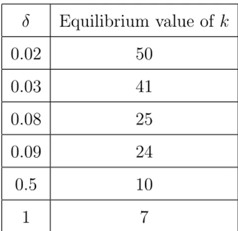
For n = 51 and various values of δ, Table 1 shows the unique value of k such that the k-candidate with simple swaps is an SSPE of the simplified ORBG.16 Recall that the payoffs induced by a k-candidate with simple swaps are given as the solutions to a system of equations which is continuous at δ = 1. Therefore, we can find the limit values as δ converges to one by considering the relevant equations forδ = 1.
For values of δ close to zero, we see that k = n −1 = 50. This exemplifies the finding in Proposition 5 that a proposal is endorsed by all players in an SSPE when discounting is sufficiently severe. As δ increases, the equilibrium value of k decreases, which is in line with Baron and Ferejohn’s findings. However, Baron and Ferejohn predict that the equilibrium value of k falls only until it reaches (n−1)/2 = 25. Again, this is because they do not take into account that players who do not endorse a proposal may still vote for it. In our model, however, the equilibrium value of k continues to fall. For δ close to one, it eventually reaches 7,which is indeed the integer close to √
n=√
51≈7.1.
δ Equilibrium value of k
0.02 50
0.03 41
0.08 25
0.09 24
0.5 10
1 7
Table 1: Equilibrium values of k for n = 51 and various values ofδ.
15The code used to simulate these examples is available from the authors upon request.
16We note that in all the numerical examples listed in the table, there is exactly one k = 1, . . . , n−1, so that thek-candidate with simple swaps is an SSPE.
8.2 Efficiency and equity for varying discount factors
One purpose of the original analysis by Baron and Ferejohn was to compare closed rule and open rule bargaining procedures with regard to the efficiency and equity of equilibrium outcomes. While open rules tend to lead to a more egalitarian distribution of the surplus, they suffer from inefficiencies. The reason is that the option of making amendments tends to lead to equilibrium delays, while closed rule bargaining models always predict immediate agreement. One important question is how one could weigh the efficiency loss against the equity gain.
We consider the example with n = 51 for different values of the discount factor. Examples 1 and 2 suggest that there is a large gain in fairness and no loss in efficiency when δ is either close to zero or close to one. However, Example 3 shows that for intermediate values ofδ, the efficiency loss from open rules can be so large that even the responding players are ex ante better off under a closed rule.
Example 1. Let us focus on the example where n = 51. First, we consider the case where δ is very small, say δ = 0.02. If players were bargaining under a closed rule, agreement would be immediate and so the surplus divided would be of size one. The proposer would “buy” 25 players’ votes by offering each of them the reservation payoff δ/n= 0.02/51<0.0004. Hence, the proposer could secure a majority by offering less than 25×0.0004 = 0.01 to other players. Under closed rule, the proposer would be able to keep more than 99 percent of the surplus for himself.
Now we turn to the case of open rule bargaining. If n = 51 and δ = 0.02, we have previously computed that k = 50. Since δ is so small, it is prohibitive for the proposer to risk bargaining delay. In equilibrium, agreement is reached immediately and the size of the surplus divided is one, just as it would be under closed rule bargaining. Substituting for n, δ, and k into Eqns. (1)-(4), we find that V50 = X50 = 0.5, while W50 = 0.01 and Y50 = 1. The equilibrium outcome under open rule can be described as follows: The proposer receives half of the surplus himself. He distributes the remaining half of the surplus equally to the other fifty players; hence, each of them receives δV50 = 0.02×0.5 = 0.01, and is
willing to endorse the proposal.
Clearly, the outcome under open rule is much more equitable than under closed rule, and equally efficient.
Example 2. Now we consider the example with n = 51 in the limit as δ → 1. First, suppose that bargaining takes place under the closed rule. In that case, the proposer needs to offer each of 25 players their reservation payoffs δ/n→1/51≈0.0196. The proposer can keep the remainder 1−25/51≈0.5098.
Now turn to the case of open rule bargaining. We have computed before that n = 51 andδ close to one give k = 7. Substituting into Eqns. (1)-(4) and solving the resulting system, we find V7 ≈0.054, W7 ≈0.0189, and X7 ≈0.2693.
Hence, under open rule, the proposer receives just over one fourth of the surplus (instead of more than a half under closed rule). Seven players receive 0.054 instead of just 0.0196.All other players obtain the same payoff under open rule bargaining as under closed rule bargaining. Indeed, the open rule bargaining leads to a more equitable, and equally efficient, outcome.
Example 3. As an example, suppose that n= 51 and δ = 0.5.With closed rule bargaining, 25 players would get the reservation payoffδ/n= 0.5/51≈0.0098.
The proposer would keep the remaining 1−25×0.0098 = 0.755.
Under open rule bargaining, we find k = 10 and the relevant system of equa- tions becomes
V10 = 0.2X10+ 0.4W10, W10 = (Y10−V10)/50,
X10 = 1−5V10−15×0.5 51 Y10, Y10 = 1/3.
Solving this system yields X10 ≈ 0.4707 and δV10 ≈ 0.048. Hence, under open rule bargaining, one would expect the proposer to receive about 0.4707 and ten players to receive 0.048. Another 15 players would receive 0.5/51 ≈ 0.0098 and the remaining 25 players would receive nothing.
However, with open rule, the expected delay is 4 and the expected surplus is 1/3. So while the outcome under open rule is certainly more equitable than under
closed rule, it is much less efficient.
Recall that V10 and W10 are the ex ante expected payoffs of the proposer and any player other than the proposer, respectively. From the above equations, we can compute V10 ≈ 0.096 and W10 = 0.0047. In a closed rule bargaining game, the analogous ex ante payoffs would be 0.755 for the proposer (since agreement is immediate) and 0.5nδ = 0.0049 for any other player. Note that ex ante, all players are better off with closed rule bargaining than with open rule bargaining forδ = 0.5.The efficiency loss from delay is so great that even the gain in fairness cannot compensate the responders for it.
9 Return to the ORBG
In previous sections, we focused on the simplified ORBG. In the present section, we return to the original ORBG, as formally defined in Section 2. Recall the crucial difference between both games: In the original ORBG, whenever a player makes an amendment to a proposal on the floor, a vote determines whether or not the amendment replaces the proposal on the floor. We will show in this section that the main results and conclusions from our analysis of the simplified ORBG carry over to the ORBG itself. To this end, we first define a set of equilibrium candidates which are analogous to the k–candidates with simple swaps in the simplified ORBG. For this definition, we first recall the system of Eqns. (1)-(4)
Vk =
k n−1
Xk+
n−1−k n−1
δWk, Wk = Yk−Vk
n−1 ,
Xk = 1−kδVk−max
0,n−1
2 −k δ
n
Yk,
Yk = k
δk+ (1−δ)(n−1).
Definition 2. Consider the ORBG G(δ, n). For every k = 1, . . . , n−1, a profile of stationary strategies is a generalized k-candidate if the following holds: