Nonperturbative physics, fractional instantons and matter ﬁelds Dissertation

(1)

Nonperturbative physics, fractional instantons and matter fields

Dissertation

zur Erlangung des Doktorgrades der Naturwissenschaften (Dr. rer. nat.) der Fakult¨ at f¨ ur Physik der Universit¨ at Regensburg

vorgelegt von

Tin Sulejmanpaˇsi´ c

aus Sarajevo, Bosnien und Herzegowina

Regensburg, Mai 2014

(2)

(3)

3

Die Promotionsarbeit wurde angeleitet von PD Dr. Falk Bruckmann.

Die Promotionskommission tagte am 16.04.2014.

Das Promotionsgesuch wurde am 15.05.2014 eingereicht.

Das Promotionskolloquium fand am 14.07.2014 statt.

Pr¨ufungsausschuss:

Vorsitzender Prof. Dr. John Lupton 1. Gutachter PD Dr. Falk Bruckmann 2. Gutachter Prof. Dr. Tilo Wettig

weiterer Pr¨ufer UnivProf. Dr. Andrea Donarini

(4)

(5)

To my daughter

May she always seek out knowledge

(6)

(7)

Introduction

The Yang-Mills (YM) theory – the theory of gluons – and quantum chromodynamics (QCD) – the theory of quarks and gluons – has had great success in the past 40+ years in describing the physics of strong interactions. These theories drew even more appeal because they are asymptotically free, a feature which allowed, in contrast to quantum electrodynamics (QED), to define the theory¹ at arbitrarily short scales and to make lattice simulations with continuum limit extrapolations.

Although seemingly perfectly tame and well behaved at short distances where perturbation theory is applicable², the theory has a very nontrivial infrared behavior which still precludes analytic treatment, exhibiting dynamical mass gap generation and confinement at large distances, phenomena not accessible in the perturbation theory. Nev- ertheless, our knowledge of nonlinear theories has significantly increased in the past decades. Asymptotically free nonlinear sigma models such as O(N) and CP(N) were

1The theory needs to be defined in a continuum and a standard way to do this is to put the theory on the lattice and let the lattice spacing run to zero. Until today this has not been done self-consistently for QED as there is a phase transition in the lattice theory when the bare coupling exceeds a certain value. Nevertheless the theory is perfectly tame when the lattice is coarse enough, i.e. it is a low energy effective theory. On the other hand YM and QCD are perfectly well defined in the ultraviolet where the coupling flows to zero. Many take the view that because of this fact QCD isfundamental while QED is not. This author takes the view that neither are fundamental (in the sense that they are the theories of nature), as we simply do not have access to experiments at sufficiently large energies and that the entire standard model can come from a fundamental theory which is quite different from either QCD or QED.

2This is perhaps a misnomer which is widely accepted. Although indeed the perturbation theory has definite applicability at short distances because of the small coupling in this regime, the perturbation series is not well defined because of the large number of diagrams which make the series non-Borel summable due to the singularities (so called ’t Hooft renormalons in Yang-Mils theory) in the Borel plane. There are examples, however, where the perturbation theory is cured by systematic resummation of the non-perturbative objects, (e.g. instanton-anti-instanton in quantum mechanics) but instantons in Yang-Mills theories did not cure the problem of these singularities. For a long time it was believed that these singularities are a sickness of the perturbation theory and cannot be cured by semi-classical objects. This view, however, is being challenged by recent progress in QCD-like theories. For recent development see [48, 19, 34, 50, 47, 49]

9

(10)

solved in the large N expansion, where a mass gap is computable and is of the form m∼e^−···/g², withg² being the bare coupling of the theory. Such a mass gap is obviously non-perturbative in the coupling and vanishes to any order in the perturbation theory.

It is very appealing to think that such a mass gap is generated by semi-classical objects with an actionS ∝1/g². Indeed instantons, classical solutions of YM equations in Euclidean space-time, were thought to be such objects. Further, because of their topological character, the Atiyah-Singer (AS)index theorem [16] guarantees that instantons have fermionic bound-states referred to as zero modes. It was discovered by ’t Hooft [106] that these bound states can be viewed as effective 2Nf fermion interactions, much like the interactions of the Nambu-Jona-Lasinio (NJL) model [76, 77]. This interaction was a welcomed surprise, as it solved the long standingU(1) problem: why there is no ninth Goldstone boson, or why is the η⁰ meson so massive. Instantons simply revealed that the U(1) axial symmetry is not spontaneously broken but is explicitly broken by instanton events. In addition it provided the desired fermion self-interaction of the appropriate symmetry which could induce spontaneous chiral symmetry breaking pattern observed in nature (i.e. light Goldstone pions).

The instantons, however, although successful in solving the U(1) anomaly problem and generating the fermion interactions required for chiral symmetry breaking, suffer from a severe problem when quantum effects are taken into account. In fact, it was shown by ’t Hooft in [106] that an instanton, although classically a scale invariant object, has an action which develops dependence on its size, reflecting the running of the coupling as a function of the typical background field size: the instanton size. The problem is that the integration over the size of the instanton is dominated by a large instanton-size contribution in the one loop approximation. This is, however, precisely the region where one-loop is not to be trusted: the elusive infrared region. As a result, a reliable semi-classical treatment of instantons, although possible under certain circumstances (e.g. in supersymmetric QCD (sQCD) [5] in the Higgs phase, and finite temperature YM/QCD theory³[57]), is impossible in QCD and YM at zero temperature.

Nevertheless, instanton phenomenology had a noted success in explaining the origin and mechanism of chiral symmetry breaking and phenomena connected to it by fixing the instanton size phenomenologically to ρ ≈ 1/3 fm (see [93] and references therein), but these models could never explain the area law and confinement. Presumably this is because they ignore the large instanton contributions which are believed, for some time now, to have something to do with confinement. Indeed it was argued a long time ago by Callan, Dashen and Gross (CDG) [31] that an instanton of large size breaks into 4D, point-like objects with fractional topological charge, which they dubbed merons.

Merons interact logarithmically, much like vortices in two dimensional theories, and can

3In the case of pure YM/QCD at finite temperature although the instanton calculus is reliable because of the one loop suppression of large instantons, the reader will note that the theory is far from solvable as there are observables which are non-calculable in perturbation theory such as the magnetic mass.

(11)

11 condense if their action cost is smaller than their entropy gain. Upon condensation of merons, CDG argued that Wilson loops will have an area law behavior. These consider- ations remain, however, purely at a phenomenological level and no rigorously calculable scenario in four dimensions based on the meron picture was found.

In the past several years non-supersymmetric YM-like theories which are under com- plete theoretical control emerged, most particularly deformed YM and QCD with quarks in the adjoint representation (QCD(adj)) [109, 98]. These theories are generically center- symmetry-preserving (confining) compactifications (as opposed to thermal compactifications) of their four-dimensional versions. Such a compactification enforces the adjoint Higgs mechanism, where, for compactification of the 4-direction, A4 plays the role of a (compact) Higgs field and the YM theory abelianizes at scales larger than the radius of compactification L. Nonetheless even though the theory is abelian at low energies, nontrivial topological objects emerge on the scene with monopole-like fields and fractional topological charge. These are instanton-monopoles discovered as constituents of instantons over a decade ago⁴ [66, 67]. They dramatically change the behavior of the theories in question, dynamically generating a mass gap and confinement. Further, instanton- monopoles have been connected to dyons, object responsible for confinement in N = 2 Super Yang-Mills (SYM) theory on R⁴, by Poisson resummation [90]. In the works of Poppitz, Sch¨afer and ¨Unsal (PSU) [87, 86] the microscopic picture of N = 1 SYM gauge theories was analyzed onR³×S¹. The partition function is well known to be the Witten index [116], which is independent of the compact radius L, so no phase transition can occur in the decompactification limit. On the other hand, PSU have shown that by breaking supersymmetry (SUSY) softly, giving an explicit, but small massm to gauginos, a confinement/deconfinement phase transition occurs of the correct order (i.e.

second for SU(2) and first for SU(N ≥ 3)) at some small compact radius L_c 1/Λ, where Λ is the strong scale of the theory. They have conjectured that this analytically tractable scenario is continuously connected to the case when m→ ∞, i.e. when gauginos are completely decoupled and the theory is pure YM. If this is indeed the case it would be a strong evidence that the same mechanism is responsible for confinement both in SYM and the pure YM theory.

In pure YM the confinement/deconfinement phase transition happens at a large radius of order L = 1/Tc ∼ 1/Λ, where Tc is the transition temperature, so that the fluctuations of the fields are large, and semiclassical analysis is not strictly applicable.

The physical interpretation of the confinement/deconfinement scenario is that in the con- fined phase, quarks are connected with a narrow electric flux tube, so that the energy of

4The credit of discovering the instanton-monopoles is often attributed to these references. However the reader will note that similar objects were discussed previously, for example in [57]. Their contribution was mostly ignored in the community as the they were thought to be irrelevant in the high-temperature phase of QCD. In [118] an attempt to compute their contribution was made, but little effort was made to understand the physics of them.

(12)

a quark–anti-quark pair is linearly growing with their distance. At high temperatures, however, thermal gluons can be excited and are able to screen the electric flux tube if the temperature is high enough. In supersymmetric theories this screening is protected by supersymmetry, where fermionic super-partners are kept periodic in the compact direction, and do not have a thermal interpretation. Because of that the would-be thermal fermions cancel the contribution of the thermal gluons. In pure YM theory this does not happen and the Polyakov loop – an order parameter of the confinement/deconfinement transition – is nonzero: the theory is in the deconfined phase. As a result the gauge field in the temporal direction is zero up to a gauge transformation, and no adjoint Higgs mechanism, which is crucial for analytical control, takes place.

Nevertheless the question “what causes confinement” in YM/QCD has been tackled by the lattice and the phenomenology community in the past years from the viewpoint of the instanton-monopoles. In the works by Ilgenfritz et. al. [59] and Bornyakov et.

al. [22] the instanton-monopoles (there referred to as dyons) were identified in lattice simulations above and below Tc. This did stir some phenomenological interest in the community [43, 40, 44] where suggestions were made that confinement is driven by the moduli space metric of instanton-monopoles⁵. A metric for the instanton-monopoles was proposed (for a review see [41] and references therein), which, apart from having a deficit of including only the self-dual sector⁶, suffered from problems at short distances of monopoles (i.e. large monopole densities) [26], so it is unclear to what extent the moduli-space metric describes the correct interactions of instanton-monopoles. On the other hand, Bruckmann et. al. [25] have shown that a random gas of instanton-monopoles is confining, while in the works [100, 51] chiral symmetry breaking was connected with randomization of instanton-monopoles, giving a potential connection between confinement and chiral symmetry breaking. Until recently this development paralleled the development in SUSY theories with little or no overlap. In our work [101] a crude model was built based on the language used in controllable theories and some comparison to lattice data was made with decent agreement.

Although a lot of work has been done in YM and its supersymmetric incarnations, a systematic understanding of the interplay between the instanton-monopoles and the fundamental fermions is still in its early infancy. Like in the case of instantons the instanton-monopoles can carry fermionic zero modes which generate ’t Hooft interactions

5The classical interactions were ignored in this argument, because the authors focused on the self-dual sector only in which instanton-monopoles do not interact. They also ignored loop effects which would generate Debye screening and make even self-dual monopoles interacting (see however next footnote).

6A suggestion on how to include the anti–self-dual monopoles was briefly discussed in [41] where a non-interaction assumption between the two sectors was made invoking electric Debye screening. It is unclear to this author why this is justified, as this would a) not eliminate the interactions between the self-dual and anti–self-dual monopoles and b) would induce interactions between the self-dual monopoles, which was absent from their analysis and the guiding reason why the authors in these works consider moduli space metric to be the leading contribution to the confinement.

(13)

13 and in principle should break chiral symmetry via a similar mechanism. In [100, 51] initial steps were taken in this directions, attempting to reconstruct the chirally broken picture of the Instanton Liquid Model. In these works, however, the detailed structure of the fermionic zero modes and interactions of monopoles via fermionic zero modes was not analyzed and only naive interactions were introduced. In addition phenomena related to finite density systems, which have eluded lattice simulations because of the infamous sign problem, must necessarily go through the fermions, so it is worthwhile to explore how the spectrum (and most importantly zero modes) changes when chemical potential is introduced. In our work [28] a detailed analysis was made of the fermionic zero modes and the so-called hopping matrix element, which is responsible for the fermion facilitated interactions between topological objects which carry zero modes.

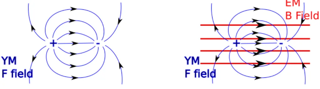
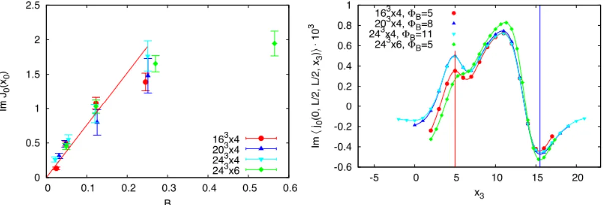
Additionally, phenomena related to strong magnetic fields are of considerable in- terests in recent years due to their possible relevance for Heavy Ion Collisions (HIC), as well as to the physics of magnetars and the early universe. Interesting effects such as Chiral Magnetic Effect [53, 63] and Chiral Separation Effect [104, 72] were found when fermions move in the background with topological charge and magnetic field. In our work [24] it was shown that a novel phenomenon happens in the background of the instanton-monopoles in magnetic field. This phenomenon was dubbedcharge catalysis as it exhibits imaginary charge⁷ accumulation in between a monopole–anti-monopole pair.

This phenomenon transcends QCD and has direct application in strained graphene.

It is of great interest to see how fundamental matter influences a theory where instanton-monopoles are important and where their computation is reliable. The most natural candidates are SUSY theories. Although extensive work has been done in the super YM case, the theories with matter where instanton monopoles appear have only gotten side (but important) remarks in generic analysis of 3D supersymmetric theories in both old and recent literature [7, 8]. Even though the addition of massless flavor multiplets renders the theory gapless and non-semiclassical, adding massive flavors al- lows semiclassical treatment and analytical control. This was the main interest of our work [88] where the one loop calculation around instanton-monopoles in supersymmetric QCD (sQCD) on R³×S¹ with heavy flavors was performed and the microscopic picture of the Polyakov loop screening and string breaking was analyzed.

Unfortunately supersymmetric theories, in addition to not being realized in nature, are much more difficult to handle at finite quark density, because the presence of the baryon charge would violate supersymmetry⁸. An O(N) model in 2D however – a com- mon toy model of non-abelian gauge theories – has a rigidSO(N) continuous symmetry and a chemical potential µ for some SO(2) ∈ SO(N) can be added. For sufficiently

7The charge being imaginary is, of course, not observable, but its effect appears in the charge-charge correlation functions. For details see Chapter 3.

8Adding an equal chemical potential to squarks does not seem to help much, because bosons and fermions have different statistics.

(14)

largeµ,SO(N) symmetry breaks toSO(2) and vortex solutions appear [4, 29] which, in the case of the O(3) model, have fractional topological charge. They can be identified as instanton constituents, i.e. instanton-monopoles, which have the ability to generate a dynamical mass gap by disordering themselves.

In this thesis we will review our works [28, 24, 88] mentioned above. We have organized the thesis as follows: In Chapter 2 we give a motivation why monopoles are important for expected infrared (IR) behavior of YM-like theories, as well as introduce notations and important results from the literature relevant for our discussions in the chapters to follow. We also review some basic facts about the O(2) model in two dimensions, vortices and the physics of the Kosterlitz-Thouless transition, and show how to introduce chemical potential in the O(N) and CP(N −1) models. In Chapter 3 we discuss the phenomenon of charge catalysis in magnetic fields, a novel phenomenon of instanton-monopoles in the magnetic field, as well as its manifestation in strained graphene. In the same chapter we discuss the explicit zero mode solutions for instanton- monopoles and calorons at finite (complex) chemical potential. Finally in Chapter 4 we discuss two dynamical models where monopole-like objects with fractional topology have a crucial influence on the IR dynamics: supersymmertic QCD onR³×S¹ and theO(N) nonlinear sigma model in two dimensional with chemical potential. In Chapter 5 we give a summary and speculate about the potential significance of instanton-monopoles in QCD and beyond.

(15)

Chapter 2

Preliminaries

This chapter deals with preliminaries which are important for the recent developments that the thesis focuses on. The chapter is organized as follows: In Section 2.1 we discuss in detail the Georgi-Glashow model which is well known to have monopoles and confinement. In Section 2.2 we review the construction of instanton-monopoles onR³×S¹ and their connection with calorons. These objects are the backbone of this thesis. In Section 2.4 the index theorem is discussed, which guarantees the existence of localized fermionic states on top of topological objects, in particular the instanton-monopoles.

In Section 2.5 some basic language, terminology and relations of supersymmetries are reviewed, which we will require later in Section 4.1.

2.1 Motivation: Georgi-Glashow model and Polyakov’s con- finement

Before we consider instanton-monopoles it is instructive to give some motivation why monopoles are important in non-abelian gauge theories. The simplest example is the SU(2) Georgi-Glashow model in 3D, i.e. an SU(2) YM + adjoint Higgs theory. We will see that this model has monopole solutions that influence the IR behavior heavily.

The Georgi-Glashow model is given by a Lagrangian density L= 1

g²₃Tr 1

2F_ij² + (Diφ)²

+V(|φ|), (2.1)

whereφ=φ^{a τ}₂^a,Diφ=∂iφ−i[Ai, φ] and|φ|=qP

a=1,2,3(φ^a)²andg²₃is the 3D coupling with the dimension of energy. If the potential V(|φ|²) has a minimum at |φ|=v, and if one makes a gauge transformation so thatφis in the 3rd color direction, the scalar field can be written as φ=v^τ₂³ + (fluctuations). Such a decomposition makes it transparent that the A^1,2µ terms in the above Lagrangian obtains the mass from the Higgs field,

15

(16)

while the A³_µ gauge field remains massless. In other words the gauge symmetry breaks spontaneously fromSU(2) to U(1).

A priori it seems that the low energy effective theory is gap-less and it is just a freeU(1) theory. However, the theory breaks to U(1) at large distances, while at short distances.1/v the fullSU(2) theory can be restored. This fact hints at the possibility that the theory can have fluctuations which are highly localized defects (i.e. appear to be singular) in the U(1) theory, but are perfectly smooth in the core because of the underlying SU(2) structure. Indeed such objects exist as solutions to the equations of motion of the Yang-Mills + adjoint Higgs theory. They were found independently by ’t Hoof and Polyakov [105, 81] and are referred to as ’t Hoof-Polyakov monopole because of their monopole character. Here we review the arguments for their existence, while we postpone their explicit solution for the next section.

To see that such objects indeed exist in the theory, it is simplest not to fix the gauge to the third color direction for the moment and just demand that the Higgs field at space-time infinity takes its expectation value, i.e. that |φ|² → v² when |r| → ∞. The space-time at infinity has a topology of a S² sphere. On the other hand, since the length of the Higgs field is constrained to be v, which is invariant under the SU(2) gauge rotations, the Higgs field at spatial infinity is a 3-vector of fixed length, and therefore also takes values on a S² sphere. The space-time at infinity to target-space Higgs field mapping is then a mapS_|r|→∞² →S_|φ|=v² . It is well known that such maps are characterized by an integer number Q ∈ Z, where Q is the so-called winding number, i.e. a number which tells us how many times does the target space sphere S_|φ|=v² get covered when we cover a sphere at space-time infinity¹ S_|r|=∞² .

Since the nonzeroQ configuration cannot be contracted continuously to trivial vacuum, such configurations must have nontrivial properties in the bulk. For our purposes it will suffice to consider the Q = 1 sector. The task now would be to find the finite action solutions of the equations of motion in this sector with Q= 1. This is however not possible analytically for arbitrary potentialV(|φ|) nor is it possible for the mexican hat potential² λ(|φ|²−v²)² . Nevertheless the most important properties of the solution can be extracted without explicit computations. The necessary condition that the action is finite is that (D_iφ)² →0 faster then 1/r³. This translates into

(Diφ)â=∂iφâ+abcA^b_iφˆ^c→v∂irˆâ+vabcA^b_iˆr^c, (r→ ∞) (2.2)

1To get an intuitive feel for the winding number it helps to think about the map fromϕ:S¹ →S¹, i.e.ϕ(α) where bothϕandαare angular variables. Since we demand thatα≡α+ 2πandϕ≡ϕ+ 2π, the maps are constrained so thatϕ(2π)−ϕ(0) = 2πQ, whereQis an integer. The maps of fixedQcannot be continuously deformed to each other without violating the boundary conditions thatα≡α+ 2πand ϕ≡ϕ+ 2π.

2It is, however, possible for the limitλ→0, i.e. the vanishing potential limit, which we discuss in the next section.

(17)

2.1. MOTIVATION: POLYAKOV’S CONFINEMENT 17 where we have assumed that φ^a ∼ vˆr^a at spatial infinity (i.e. we assumed spherical symmetry). Asymptotically the covariant derivative of the Higgs field is given by

(Diφ)â∼vδâi−rˆâˆrⁱ

r +vabcA^b_irˆ^c. (2.3) The above combination must vanish at infinity because the first term above decays too slowly for the action to be finite (i.e. as 1/r so that its square, which is 1/r², would give a linear IR divergence of the action). It is easy to see that this asymptotic equation is solved byA^b_i = ¹_r_bikˆr^k. Computing the asymptotic field strength gives that Bâ_i = ¹₂îjkF_jkâ ∼ −^r^ˆⁱ_r^r^ˆ²â. Notice that the asymptotic field is in the same color direction as the Higgs field, i.e. that B_iâφâ ∼ −_r^r^ˆ²ⁱ. This is as it should be as we said that the long range theory is a U(1) theory, where the U(1) subgroup was selected by the Higgs vacuum expectations value (VEV). So we have a field of a (anti-)monopole³!

Since the couplingg²₃has dimensions of energy, and since the only scale in the problem is v, we must have that the classical action of the monopole solution is of the form

S=c v

g₃² . (2.4)

where c is some dimensionless constant. This will suffice to illustrate the important points.

Now that we have found the asymptotics of the solution, we must find the way how to incorporate them into the effective theory. Firstly we must understand how to integrate over such configurations. Let us say that we want to include a monopole at positionx₀ in the path integral. Then we would write the gauge field as A_i =A^mon_i (x₀) +a_i where ai are the fluctuations around the monopole solution. Heuristically we expect that the integration measure should change as follows

Z

DA_i→ Z

Da_i Z

d³x₀ (2.5)

so that integration breaks into distinct parts, one of fluctuation around the monopole at point x0 and the other the integration over all monopole positions.

Indeed this is what will happen. The details of how this decomposition occurs are given in Appendix C.1. However the integration over the so called collective coordinates x0 clearly must be accompanied by a dimensionfull metric gij which will render the integration measure√gd³x0dimensionless. We will not worry about this at the moment, instead we leave a more precise treatment for the case of four dimensional YM theory, where similar objects appear. It will suffice to say that this metric is constant for a

3Whether it is a monopole or an anti-monopole will depend on the sign ofv.

(18)

single monopole and does not depend on⁴ x0 because of translational invariance. For now we will simply include a constantC with any integration overd³x0.

The obstacle now is to account for the interactions between multiple monopoles.

These interactions will, unsurprisingly, be coulomb-like because of the long range abelian fields. It is not difficult to show⁵that the interaction action between a monopole located atr₁ and an (anti-)monopole located atr₂ is

Sint(|r1−r2|) =±1 g²₃

4π

|r1−r2| (2.6)

where the upper sign refers to the like charges (i.e. two monopoles, or two anti- monopoles) and the lower sign refers to the unlike charges (i.e. monopole and anti- monopole). The partition function of the monopole gas would then have to include these long range interactions.

In 1976 Polyakov [83] devised an ingenious duality by noticing that the interactions can be accounted for by introducing a scalar fieldσ with the kinetic term S[σ] = Rd³x _2(2π)^g²³ 2(∂iσ)². The (anti-)monopole at positionx0 would then couple to theσ field in the following fashion

monopole operator∝e^±iσ(x⁰⁾. (2.7) Indeed it takes little effort to show that

Z

Dσ e^iσ(r¹⁾e^±iσ(r²⁾e^−S[σ]∝e^∓

4π g2

3|r1−r2| =e^−S^int^(|r¹^−r²^|) (2.8) The effective U(1) theory we want to describe would then have a dual description in terms of the free Lagrangian

L^{f ree}dual = g²₃

2(4π)²(∂_iσ)². (2.9)

There is a more formal way of showing the above duality. Indeed because of the Higgs

4For multiple monopoles the metric gets corrections which depend on the distances between monopoles. These corrections, however, can be neglected for dilute regimes, which is what we will discuss. The reader is however advised that in pure YM theory in 4D these “moduli space interactions”

might be important, as was argued in some models based on instanton-monopoles [40] (see also [41])

5The total asymptotic chromo-magnetic field of the two monopoles is given byB = B1 +B2 =

ˆ r₁ r²₁

τ³ 2 +^ˆ^r_r²2

2 τ³

2, where r1, r2 are distances from the monopole centers to the observation point and ˆr1,rˆ2

are unit vectors pointing from the monopoles to the observation point. Since the action is g²S = Rd³xtrB²₁+R

d³xtrB²₂+ 2R

d³xtrB1·B2+. . ., where the dots stand for Higgs field action which, because of the Higgs mass does not contribute to the interaction between monopoles. The first two terms do not depend on the distance between monopoles and they combine with the Higgs action to make 2S0, while the third term yields (neglecting irrelevant core-contribution)g²₃Sint= 2R

d³xtrB1·B2=_|r^4π

1−r₂|

(19)

2.1. MOTIVATION: POLYAKOV’S CONFINEMENT 19 mechanism which gives two out of three gluons a mass (i.e. they become heavy W bosons) the YM part of the SU(2) action becomes _2g¹2

3

trF_ij² → _4g¹²

3F^ij, whereF^ij =∂iA^j−∂jAⁱ is the abelian field strength, and Ai is the gauge field which remained mass-less (e.g.

Ai =A³_i in the gauge wherehφi=v^τ₂³). In writing this we have simply integrated over the massive W-bosons which are short ranged (of order∼1/v) and will not contribute to the long-distance dynamics.

The partition function is then an integral over the mass-less gauge field Ai only.

However, this is equivalent to integrating over the field-strength Fij and imposing the Bianchi identity ^ijk∂iFjk = 0. We therefore have

Z

DAi e⁻

1 4g2

3

Rd³xF_ij²[A]

= Z

DFij e⁻

1 4g2

3

Rd³xF_ij²

δ(^ijk∂_iFjk) =

= Z

DFij

Z

Dσ e⁻

1 4g2

3

Rd³xF_ij²+i_8π¹ R

d³x ^ijk∂iσF_jk

= Z

Dσ e⁻

g2 3 2(4π)2

Rd³x(∂iσ)²

. (2.10) In the above we introduced a term _8πⁱ σ^ijk∂iFjk in the Lagrangian, which upon integration over the Lagrange multiplierσ imposes the Bianchi identity. This allowed us to integrate over the field strength Fij generating a theory which depends only on the σ field. The theory we ended up with is a theory of the scalar field σ only. The Bianchi constraint is precisely the condition that there are no monopoles. However, inserting a (anti-)monopole at positionx₀ is as simple as inserting an operatore^±iσ(x⁰⁾. Indeed by integrating over theσ field with the insertion of this operator it is easy to see that the constraint is now ¹₂^ijk∂iFjk =∇·B = 4πδ(x−x0), which corresponds to a monopole atx₀.

We are ready now to include many monopoles and anti-monopoles into the partition function. Firstly we go to a dual description in terms of the σ field with the kinetic Lagrangian _2(4π)^g²³ 2(∂_iσ)². Including monopoles means integrating over monopole- like configurations and so each monopole should be weighted by a factor e^−S⁰^±σ(x⁰⁾, where σ(x₀) accounts for the magnetic charges, and then integrated over the moduli- space metricR

d³x0C. The partition function in the dual description accounting for the monopoles can then be written as

Z = Z

Dσ e⁻

g2 3 2(4π)

Rd³x¹₂(∂iσ)²

× X∞

M=0

1 M!

Z

d³x0 Ce^−S⁰^+iσ(x⁰⁾

M X∞

M¯=0

1 M!¯

Z

d³x0 Ce^−S⁰^−iσ(x⁰⁾ M^¯

=

= Z

Dσ e⁻

g2 3 2(4π)

Rd³x(¹₂^(∂iσ)²−m²cosσ) (2.11)

(20)

where the second line accounts for monopoles (sum over M) and anti-monopoles (sum over ¯M) which exponentiated and formed a cos(σ) potential for the σ field with m² =

2(4π) g₃² C.

So what happened here? An effective U(1) theory dual to a free scalarσ-field theory, which without monopoles had no potential for the scalar field σ, has, upon monopole resummation, obtained a potential, and, therefore, the massmfor theσfield. That this happened is not horribly surprising once we think about the physics of this mechanism.

Because of its three-dimensional nature, the effective theory was a free theory of U(1)

“magnetic field” only⁶ (i.e. Lef f ∝B²). Without monopoles the magnetic interactions would be long ranged and decay non-exponentially. Introduction of monopoles in the theory changes this qualitative picture completely. Since monopoles are able to screen the magnetic field by redistributing themselves appropriately in the vacuum, the correlation functions become exponential. This is known as themagnetic Debye screening⁷.

To make this more explicit let us consider a Wilson loop observable i.e.

W[C] =

tr exp(iτ³ 2

I

C

dxⁱAi)

(2.12) whereC is some contour. Notice the factor ofτ³/2 in the exponent. This is due to the fact that we consider quarks in fundamental representation. The above observable is diagonal in color and can be computed by first evaluating

exp(i1

2 I

C

dxⁱAi)

=

exp(i1 2

Z

S

dSi Bⁱ

(2.13) where dS_i is a surface element and the integration is over a surface S such that its boundary isC, i.e. C=∂S andBⁱ = ¹₂^ijkFjk is the abelian magnetic field. Let us take a contour C lying entirely in the x1, x2 plane, and let us take the surface S also in the (x₁, x₂) plane. Then inserting the above operator in the Lagrangian (2.10) containing both σ and Fij fields, integrating over Fij and summing over (anti-)monopoles we get the following action

L^W−loop_dual = g₃² 2(4π)²

"

∂_kσ+ 2πδ(x₃)θ(x₁, x₂)δ_k,32

−m²cosσ

#

(2.14) whereθ(x1, x2) = 1 forx1, x2 ∈S and zero otherwise. The above action is infinite unless

6What we call here “magnetic field” is perhaps misleading. Namely we think of the three-dimensional problem at hand as a static four-dimensional one. In that sense the Fij are simply magnetic field components. Note however that this analogy is incomplete as static electric charges should also exist in a truly four-dimensional problem. This will indeed be the case in four-dimensional theories which we discuss later on.

7This is not to be confused to theelectricDebye screening, responsible for deconfinement.

(21)

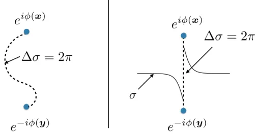
2.1. MOTIVATION: POLYAKOV’S CONFINEMENT 21 the term in the parenthesis is a smooth function across the surface S, i.e. we demand that

∂₃σ+ 2πδ(x₃)θ(x₁, x₂) = (smooth function). (2.15) The above condition translates into

σ(x3 = 0⁺)−σ(x3 = 0⁻) =−2π (2.16) i.e. the σ field has a jump across the surface whose boundary is the contour C. This means that σ field is a periodic field with a period 2π. This is the crucial difference between a SU(2) theory and a SO(3) theory, where integer charges would be allowed, and σ field would have a 4π period. (For more details discussing this difference see e.g.

[10].)

Let us now solve the classical equations of motion in the presence of the Wilson loop.

The equations of motion from (2.14) are

−2∂_k(∂_kσ+ 2πδ(x3)θ(x1, x2)δ_k3) +m²sinσ= 0. (2.17) For a large surface S we can look for a solution which only depends on x₃. Since we need to make a jump by 2π atx3= 0 we take the following solution⁸

σ =

( 4 arctan(e^−mx³^/

√2) x₃ >0

−4 arctan(e^mx³^/

√

2) x3 <0 (2.18)

The form above hasσ →0 forx→ ±∞ and has the appropriate jump of 2π across the surface. The action of the above configuration can be computed and is

S ≈ g₃²m 2√

2π²A+Svac (2.19)

where A is the area and where we ignored potential edge corrections and S_vac is the action of the vacuum (i.e. cosσ = 1, ∂iσ = 0). The average expectation value of the

Wilson loop is then

eⁱ^τ

3 2

HAidxⁱ

≈2e⁻

g2 3m 2π2A

(2.20) which is the famous area law.

We conclude this section by summarizing the important points:

8The solution is found for x3 6= 0 by multiplying the equation of motion −2∂3²σ+m²sinσ = 0 by ∂3σ and integrating over sigma we get that (∂3σ)²+m²cosσ = const. Since we must have that for x3 → ±∞ the Lagrangian (2.14) goes to the vacuum cosσ = 1 and ∂3σ = 0, then we have σ = 4 arctan(e^±m(x³^−x⁰³^)/

√

2) + 2πk=±arctan(e^m(x³^−x⁰³^)/

√

2) + 2πk⁰, where k, k⁰ are integers, andx⁰3 is an integration constant.

(22)

• The Georgi-Glashow model in the color broken phase is analytically tractable

• The low energy effective theory is aU(1) theory with monopoles

• It exhibits nontrivial IR behavior such as the mass the gap generation and the area law

The crucial component in the non-trivial IR behavior of the theory were magnetic monopoles. The natural question now whether similar objects exist 4D theories. Al- though there are no such solutions known on⁹ R⁴, we shall see in the next section that similar objects do appear in theories defined on R³×S¹.

2.2 Monopoles and calorons on R

³

× S

¹

In this section we describe in detail the construction of instanton-monopoles onR³×S¹ and explain their connection to instantons. These objects will be the backbone of the chapters to come and around which the entire thesis revolves. Various discussions in this section can be found in [41, 99, 66], but the reader will keep in mind that there are powerfulD-brane arguments of their existence which are well worth exploring [68] (for a pedagogical introduction intoD-branes and their connection with self-dual solutions see [108]).

2.2.1 The BP S monopole

We start with the dimensional reduction of the 4D Yang-Mills theory, which has the Lagrangian

L= 1

2trF_ij² + tr (DiA4)² (2.21) where we have ignored the field dependence on thex4-component and where the covariant derivative acts in the adjoint representation, i.e. as¹⁰ D_i = ∂_i −i[A_i, ]. The above Lagrangian is reminiscent of the Georgy-Glashow Lagrangian (2.1) with a vanishing Higgs potential. The equations of motion are

D_iF_ij = 0, D_i²A₄ = 0. (2.22)

9A popular mechanism of confinement onR⁴ is ’t Hooft’s abelian projection [107]. The monopoles there, however, appear as gauge-dependent objects. Although they have been very important in phenomenology of QCD and pure YM, we do not discuss these here.

10We always assume, unless otherwise specified, that the generators are in the fundamental representation.

(23)

2.2. MONOPOLES AND CALORONS ON R³×S¹ 23 These are second order nonlinear differential equations which are difficult to solve. How- ever it is possible to simplify the problem by considering a positive definite quantity

0≤ 1 g²

Z

d⁴xtr (DiA4±1

2^ijkFjk)² =

= 1 g²

Z

d⁴xtr

(DiA4)²+1

2F_ij² ±^ijkDiA4Fjk

=S± 8π²

g² Q (2.23) whereS is the action, and Q= _32π¹2^µνρσR

d⁴xtr (FµνFνρ) =_8π¹2^ijkR

d⁴xtr (DiA4F_jk) is the topological charge (see Appendix B). The above equation implies that

S ≥ 8π²

g² |Q|. (2.24)

In other words the lower bound of the action is not zero, but depends on its topological chargeQ. We can look for the solutions which saturate the lower bound. These solutions were found by Prasad and Sommerfield [91] and independently by Bogomolny [21] and are known as Bogomol’nyi-Prasad-Sommerfield (BPS) solutions and their equations are often referred to as self-duality equations

DiA4 =±1

2_ijkF^jk (2.25)

The equations of motion (e.o.m.) can be solved by the following spherically symmetric ansatz

Aâ_i =A(r)aijrˆ^j , Aâ₄ =H(r) ˆrâ (2.26) where A(r),H(r) are functions of the radial component r only. The above ansatz is motivated by the same reasoning as in the previous section (see eqs. (2.2-2.3) and the text below them). Since we are interested in the solutions in the abelian vacuum, we take H → v =±|v|,(r → ∞) where, as we shall see, the sign will depend on whether the solution is self-dual or anti–self-dual.

We have

(D_iA₄)^a=δ^ia H

r − HA

+ ˆrⁱrˆ^a

H⁰+HA −H r

(2.27)

∂iA^a_j =

A⁰− A r

ˆ

rⁱajkrˆ^k+A

raji (2.28)

−i[Ai, Aj]â=ijkrˆ^kˆrâA² (2.29) îjkF_jkâ = 2

A⁰−A r +A²

ˆ

rⁱrˆ^a−2δ^ia

A⁰+A r

(2.30)

(24)

or, takingA= (1−A(r))/r

E_iâ= (D_iA₄)â= ˆrⁱrˆâ−δîa

−HA r

+ ˆrⁱrˆ^aH⁰ (2.31a) B_i^a= 1

2_ijkF_jkâ = ˆrⁱˆrâ−δîa

−A⁰ r

+ ˆr^arˆⁱ

A²−1 r²

(2.31b) The tensors (δîa −rˆⁱrˆâ) and ˆrⁱrˆâ are orthogonal to each other, therefore demanding (anti–)self-duality E_iâ=±B_iâ and identifying the corresponding tensor factors we must have

A⁰ =±HA H⁰ =±A²−1

r² (2.32)

Since we demand thatH(r→ ∞) =v, from the first equation we have that theA∼e^±vr asymptotically, so that we must takev=−|v|for self-dual and v=|v|for anti–self-dual solution in order to avoid A blowing up at infinity. Plugging into the second equation, we see that the Higgs field must asymptote asH ∼v∓¹_r, so we write H(r) =h(r)∓ ¹_r and alsoa(r) = ^A(r)_r . The above equations simplify to

a⁰(r) =±ha (2.33)

h⁰(r) =±a² (2.34)

From the ratio of these two equations we can easily get that h² =a²+const. Since a is zero asymptotically we must have h² =a²+v² or that a² =h²−v². Substituting in the second equation we obtain

h⁰(r) =±(h²(h)−v²)→h(r) =±vcoth(vr) (2.35) Where the integration constant was chosen so that H =h± ¹_r =± ¹_r −vcoth(vr)

is regular atr = 0. Sincea(r)² =h(r)²−v² we get

a= v

sinh(rv) (2.36)

Finally we have that H=±

1−vrcoth(vr) r

, A= 1

r − v

sinh(rv) (2.37) The positive and negative signs correspond to the self-dual and anti–self-dual solutions.

(25)

2.2. MONOPOLES AND CALORONS ON R³×S¹ 25 Now let us compute the asymptotic fields. From (2.31) we have that

E_i^a≈ ∓ˆrⁱrˆ^a 1

r² B_i^a≈ −rˆ^arˆⁱ 1

r² . (2.38a)

The upper solution is obviously self-dual and the lower anti–self-dual. Projecting onto the Higgs field ˆφ^a=∓ˆr^awe see that the self-dual solution has monopole-like asymptotics and anti-self–dual anti-monopole-like asymptotics.

2.2.2 The KK monopole

In the previous section we constructed the BP S monopole in Yang-Mills theory on R³×S¹. This monopole is a three-dimensional object, i.e. completely static in “time”

x₄, and it exists in the Georgi-Glashow model as well.

However due to the fact that the theory is locally four-dimensional, there exists another solution which carries a twist in the 4-direction. Because of this twist the monopole is referred to as the Kaluza-Klein (KK) monopole.

Before we explain how to construct this monopole, let us first discuss our choice of gauge. Namely in the previous section we constructed the monopole in the radial gauge, where the Higgs field had a hedgehog r dependence, i.e. A^a₄ ∝rˆ^a. This gauge is convenient for constructing the solution, but it is utterly bad for considering an ensemble of many (anti-)monopoles, the reason being is that in this gauge the monopole center is a special point. It is much more convenient to rotate the Higgs field so that it takes one color direction, for example the 3-direction, so thatA4 ∝ ^τ₂³. This is always possible by an appropriate x₄-independent gauge transformation, at the cost of introducing Dirac strings¹¹where the gauge field is not defined¹². The multi-monopole solution would then consist of (anti-)monopoles which have the same asymptotics of the compact Higgs field A₄.

So far we have seen that there are BPS monopoles and BPS anti-monopoles which, in the radial gauge, differed by whether the “Higgs” field winds in the positive or negative direction, i.e. taking v >0 whetherAâ₄ ∝vˆrâ orφâ∝ −vˆrâ asymptotically. To classify objects which exist with the same holonomy asymptotics (up to a gauge transformation) we must go to a gauge where the asymptotic Higgs fieldA₄ does not depend on the posi- tion of the monopoles. To that end let us apply a x4-independent gauge transformation

11These Dirac strings will appear in the caloron solution which is comprised out of a monopole and an anti-monopole, as we shall see.

12Strictly speaking one would have to have two patches of gauge field in order to describe aU(1) Dirac monopole field [46].

(26)

which rotates the color direction ˆr·τ intoτ³ and −τ³, i.e.

U₊^†ˆr·τU₊=τ³ (2.39)

U₋^†ˆr·τU−=−τ³ (2.40)

The explicit forms of matrices U± can be found in e.g. [41], but we omit them since they are irrelevant for our discussion. If we apply theU+ gauge transformation above to the solutions with theAâ₄ ∝ˆrâ andU− transformation to the solution withAâ₄ ∝ −rˆâ we have that the asymptotic fields of both monopole and anti-monopole is the same, i.e.

we have that asymptotically

A^a₄ ∼vδ^a3 (2.41)

This gauge is known as the abelian gauge or sometimes the stringy gauge because it introduces Dirac string singularities in the gauge field.

Now we ask a question: could we construct other solutions which have the same asymptotic behavior of the Higgs field but are different solutions? The answer is affir- mative, as is seen by doing the following. Take a BPS solution of the previous section and replace the parameterv by

¯

v= 2π/L−v , (2.42)

so that the asymptotic Higgs field A4 has the behavior A^a₄ ∼ ¯vˆr^a. Such a solution has topological chargeQ= ^¯^vL_2π.

Now take the gauge transformationU−discussed above. The asymptotic Higgs field becomes

A₄ ∼¯vrˆ·τ

2 →A⁰₄ =U₋^†A₄U− ∼ −¯vτ³

2 . (2.43)

Next we can take the x₄-dependent gauge transformation V(x₄) = e⁻ⁱ^πx^L⁴^τ³. Notice that this gauge transformation is anti-periodic, i.e. that V(0) = −V(L). Since the gauge fields are in the adjoint representation, they will remain periodic and this gauge transformation is allowed¹³. The gauge transformation acts on the Higgs as

A⁰₄ ∼ −¯vτ³

2 →A⁰⁰₄ =V^†A⁰₄V +V^†∂4V ∼vτ³

2 . (2.44)

We have found a new solution which has the same asymptotic in the abelian gauge as our two original BPS solutions! The cost of constructing such a solution was to introduce a x4-dependent gauge twist in a solution with the parameter ¯v = 2π/L−v. This gauge twist does not affect the asymptotics of the gauge fields, as it is solely in the unbroken

13The same is not true for fermions in the fundamental representation, which has a great consequence on whether or not the monopole solution has a fermionic zero mode. We will discuss these issues in Section 2.4