characterization of the one-mode case
David Davalos,
1Camilo Moreno,
2Juan-Diego Urbina,
2and Carlos Pineda
11
Instituto de F´ısica, Universidad Nacional Aut´ onoma de M´ exico, M´ exico
∗2
Institut f¨ ur Theoretische Physik, Universit¨ at Regensburg, D-93040 Regensburg, Germany
We study one-mode Gaussian quantum channels in continuous-variable systems by performing a black-box characterization using complete positivity and trace preserving conditions, and report the existence of two subsets that do not have a functional Gaussian form. Our study covers as particular limit the case of singular channels, thus connecting our results with their known classi- fication scheme based on canonical forms. Our full characterization of Gaussian channels without Gaussian functional form is completed by showing how Gaussian states are transformed under these operations, and by deriving the conditions for the existence of master equations for the non-singular cases.
PACS numbers: 03.65.Yz, 03.65.Ta, 05.45.Mt
I. INTRODUCTION
Within the theory of continuous-variable quantum sys- tems (a central topic of study given their role in the description of physical systems like the electromagnetic field [1], solids and nano-mechanical systems [2] and atomic ensembles [3]) the simplest states, both from a theoretical an experimental point of view, are the so- called Gaussian states. An operation that transforms such family of states into itself is called a Gaussian quan- tum channel (GQC). Even though Gaussian states and channels form small subsets among general states and channels, they have proven to be useful in a variate of tasks such as quantum communication [4], quantum com- putation [5] and the study of quantum entanglement in simple [6] and complicated scenarios [7].
Writing Gaussian channels in the position state repre- sentation is often of theoretical convenience, for instance for the calculation of position correlation functions. Thus an obvious way to proceed is to characterize the possible functional forms of GQC in such representation. First at- tempts in this direction were given in Ref. [8], but their ansatz is limited to only Gaussian functional forms (de- noted simply by Gaussian forms or GF). Going beyond such restrictive assumption, in the present work we char- acterize another two possible forms that can arise directly from the definition of Gaussian channel in the one-mode case. We thus give a complete characterization of GQC in position state representation, and study the special case of singular Gaussian quantum channels (SGQC), i.e. the operations for which the inverse operation doesn’t exist.
The paper is organized as follows. In section II we discuss the definition of GQC and introduce functional forms beyond the GF that emerge from singularities in the coefficients that define a GQC with GF. In section III we give a black-box characterization of such channels, us- ing complete positivity and trace preserving conditions.
∗davidphysdavalos@gmail.com
In section IV we study functional forms that lead to SGQC and derive their explicit form. Finally in section V we derive conditions of existence of master equations and their explicit forms. We conclude in section VI.
II. GAUSSIAN QUANTUM CHANNELS Gaussian states are characterized completely by first (mean) and second (correlations) moments encoded in the mean vector d ⃗ and the covariance matrix σ. There- fore, a Gaussian state S can be denoted as S = S (σ, d), ⃗ where for the one-mode case we have
σ = ( ⟨ˆ q
2⟩ − ⟨ˆ q⟩
2 12⟨ˆ q p ˆ + pˆ ˆ q⟩ − ⟨ˆ q⟩⟨ˆ p⟩
1
2
⟨ˆ qˆ p + pˆ ˆ q⟩ − ⟨ˆ q⟩⟨ˆ p⟩ ⟨ˆ p
2⟩ − ⟨ˆ p⟩
2) , and
d ⃗ = (⟨ˆ q⟩, ⟨ˆ p⟩)
Twith ˆ q and ˆ p denoting the standard position and momen- tum (quadrature) operators [9].
To start with, we recall the following definition [10]:
Definition 1 (Gaussian quantum channels). A quantum channel is Gaussian (GQC) if and only if it transforms Gaussian states into Gaussian states.
This definition is strictly equivalent to the statement that any GQC, say G, can be written as
G [ρ] = tr
E[U (ρ ⊗ ρ
E) U
†] (1) where U is a unitary transformation, acting on a com- bined global state obtained from enlarging the system with an environment E, that is generated by a quadratic bosonic Hamiltonian (i.e. U is a Gaussian unitary) [10].
The environmental initial state ρ
Eis a Gaussian state and the trace is taken over the environmental degrees of freedom.
Following definition 1, a GQC is fully characterized by its action over Gaussian states, and this action is in
arXiv:1902.07163v1 [quant-ph] 19 Feb 2019
turn defined by affine transformations [10]. Specifically, G = G (T, N, ⃗ τ) is given by a tuple (T, N, τ) ⃗ where T and N are 2 × 2 real matrices with N = N
T[10] acting on Gaussian states according to G (T, N, τ ⃗ ) [S (σ, d)] = ⃗ S (TσT
T+ N, T d ⃗ + ⃗ τ). In the particular case of closed systems we have N = 0 and T is a symplectic matrix.
Let us note that although channels with Gaussian form trivially transform Gaussian states into Gaussian states, the definition goes beyond GF. Introducing difference and sum coordinates, x = q
2− q
1and r = (q
1+ q
2)/2, and ρ(x, r) = ⟨r −
x2∣ ρ ˆ ∣r +
x2⟩, a quantum channel
ρ
f(x
f, r
f) = ∫
R2
dx
idr
iJ (x
f, x
i; r
f, r
i)ρ
i(r
i, x
i) , (2) maps an initial ˆ ρ
iinto a final ˆ ρ
fstate linearly through the kernel J(x
f, x
i; r
f, r
i). In order to see how a chan- nel without GF can be constructed as a limiting case of a quantum channel with GF, consider the general parametrization of the later as given in [12]
J
G(x
f, x
i; r
f, r
i) = b
32π exp [ı(b
1x
fr
f+ b
2x
fr
i+ b
3x
ir
f+ b
4x
ir
i+ c
1x
f+ c
2x
i) − a
1x
2f− a
2x
fx
i− a
3x
2i], (3) where all coefficients are real and no quadratic terms in r
i,fare allowed. Now it is easy to see that if the co- efficients of the quadratic form in the exponent of J in eq. (3) depend on a parameter such that for → 0 they scale as a
n∝
−1and b
n∝
−1/2, then
lim
→0J
G(x
f, x
i; r
f, r
i) = N δ(αx
f−βx
i)e
Σ′(xf,xi;rf,ri), (4) where α, β ∈ R and Σ
′(x
f, x
i; r
f, r
i) is a quadratic form that now admits quadratic terms in r
i,f. This is the first example of a δGQC, namely a Gaussian quantum channel that contains Dirac-delta functions in its coordi- nate representation. This particular example is not only of academic interest. Physically, it can be implemented by means of the ubiquitous quantum Brownian motion model for harmonic systems (damped harmonic oscilla- tor) [13]. In such system δGQC occur at isolated points of time, defined in the limit of the antisymmetric position autocorrelation function tending to zero.
Since the form of eq. (4) admits quadratic terms in r
i,f, it suggest that a form with two deltas can exist and can be defined with an appropriate limit. In order to avoid working with such limits, in this work we provide a black-box characterization of general GQCs without Gaussian form. In particular we study channels that can arise when singularities on the coefficients of Gaussian forms GF occur, that lead immediately to singular Gaus- sian operations. We characterize which forms in δGQC lead to valid quantum channels, and under which condi- tions singular operations lead to valid singular quantum channels (SGQC). We will show that only two possible forms of δGQC hold according to trace preserving (TP) and hermiticity preserving (HP) conditions. The chan- nel of eq. (4) is one of these forms, as expected. Later on
we will impose complete positivity in order to have valid GQC, i.e. complete positive and trace preserving (CPTP) Gaussian operations, going beyond previous characteri- zations of GQC [12].
III. COMPLETE POSITIVE AND TRACE-PRESERVING δ−GAUSSIAN
OPERATIONS
Let us introduce the ans¨ atze for the possible forms of GQC in the position representation, to perform the black-box characterization. Following eq. (1) and taking the continuous variable representation of difference and sum coordinates, the trace becomes an integral over posi- tion variables of the environment. Then we end up with a Fourier transform of a multivariate Gaussian, having for one mode the following structures: a Gaussian form eq. (3), a Gaussian form multiplied with one-dimensional delta or a Gaussian form multiplied by a two-dimensional delta. Thus, in order to start with the black-box charac- terization, we shall propose the following general Gaus- sian operations with one and two deltas, respectively
J
I(x
f, r
f; x
i, r
i) = N
Iδ( ⃗ α
T⃗ v
f+ ⃗ β
Tv ⃗
i)e
Σ(xf,xi;rf,ri), (5) J
II(x
f, r
f; x
i, r
i) = N
IIδ(A⃗ v
f− B⃗ v
i)e
Σ(xf,xi;rf,ri), (6) where the exponent reads
Σ(x
f, x
i; r
f, r
i) = ı(b
1x
fr
f+ b
2x
fr
i+ b
3x
ir
f+ b
4x
ir
i+ c
1x
f+ c
2x
i+ d
1r
f+ d
2r
i)
−a
1x
2f− a
2x
fx
i− a
3x
2i− e
1r
2f− e
2r
fr
i− e
3r
2i, (7)
⃗ v
i,j= (r
i,j, x
i,j) and N
I,IIare normalization constants.
They provide, together with eq. (3) all possible ans¨ atze for GQC. Note that the coefficients in the exponential of every form must be finite, otherwise the functional form can be modified.
Let us study now CPTP conditions, since complete pos- itivity implies positivity and in turn it implies hermiticity preserving (HP). For sum and difference coordinates HP reads
J (−x
f, r
f; −x
i, r
i) = J (x
f, r
f; x
i, r
i)
∗. (8) Following this equation, it is easy to note that the coef- ficients a
n, b
n, c
n, e
nmust be real with d
n= 0, as well the entries of matrices (and vectors) A, B, α, ⃗ β. The ⃗ factor concerning the delta function of eq. (5), is reduced into two possible combinations variables: i) δ(αx
f− βx
i) and ii) δ(αr
f−βr
i). For the case of eq. (6), the prefactor concerning the two-dimensional delta is reduced to iii) δ(γr
f− ηr
i)δ(αx
f− βx
i). Let us now analyze the trace preserving condition (TP), which for continuous variable systems reads
∫
R
dr
fJ (x
f= 0, r
f; x
i, r
i) = δ(x
i). (9)
This condition immediately discards ii) from the above combinations of deltas, thus we end up with cases i) and iii). For case i) TP reads
N
I∫ dr
fδ(−βx
i)e
Σ= N
I∣β∣
√ π e
1δ(x
i)e
e2 2r2
i
4e1
e
−e3ri2, (10) thus the relation between the coefficients assumes the form
e
224e
1− e
3= 0, (11)
and the normalization constant N
I= ∣β∣ √
e1
π
with β ≠ 0 and e
1> 0. For case iii) the trace-preserving condition reads
N
II∫ dr
fδ(γr
f− ηr
i)δ(−βx
i)e
Σ= N
II∣βγ∣ δ(x
i)e
−e1(γη)2r2i−e2ηγr2i−e3r2i. Thus the following relation between e
ncoefficients must be fulfilled
e
1⎛
⎝ η γ
⎞
⎠
2
+ e
2η
γ + e
3= 0, (12) with γ, β ≠ 0 and N
II= ∣βγ∣. In the particular case of η = 0, eq. (12) is reduced to e
3= 0. As expected from the analysis of limits above, we showed that δGQC admit quadratic terms in r
i,j.
Up to this point we have hermitian and trace preserv- ing Gaussian operations; to derive the remaining CPTP conditions, it is useful to write Wigner’s function and Wigner’s characteristic function, which we now derive.
The representation of the Wigner’s characteristic func- tion reads
χ(⃗ k) = tr[ρD(⃗ k)]
= exp [−
1 2
k ⃗
T(ΩσΩ
T) ⃗ k − ı (Ω⟨ˆ x⟩)
T⃗ k] (13) and its relation with Wigner’s function
W (x ) = ∫
R2
d⃗ xe
−ıx⃗TΩ⃗kχ (⃗ k) (14)
= ∫
R
e
ıpxdx ⟨r − x 2 ∣ ρ ˆ ∣r +
x
2 ⟩. (15) where ⃗ k = (k
1, k
2)
T, x ⃗ = (r, p)
Tand ̵ h = 1 (we are using natural units). Using the previous equations to construct Wigner and Wigner’s characteristic functions of the ini- tial and final states, and substituting them in eq. (2), it is straightforward to get the propagator in the Wigner’s characteristic function representation
J ˜ (⃗ k
f, ⃗ k
i) = ∫
R6
dΓK(⃗ l)J (⃗ v
f, ⃗ v
i), (16)
where the transformation kernel reads K(⃗ l) = 1
(2π)
3e
[ı(kf2rf−kf1pf−ki2ri+ki1pi−pixi+pfxf)], with
dΓ = dp
fdp
idx
fdx
idr
fdr
iand
⃗ l = (p
f, p
i, x
f, x
i, r
f, r
i)
T.
By elementary integration of eq. (16) one can show that for both cases
J ˜
I,III(⃗ k
f, ⃗ k
i) = δ (k
1i− α
β k
f1) δ (k
2i− ⃗ φ
TI,III⃗ k
f) e
PI,III(⃗kf), (17) where P
I,III(⃗ k
f) = ∑
2i,j=1P
ij(I,III)k
fik
fj+∑
2i=1P
0i(I,III)k
ifwith P
ij(I,III)= P
ji(I,III). For case i) we obtain
P
11(I)= − ((
α β )
2
(a
3+ b
234e
1) + α β (a
2+
1 2
b
1b
3e
1) + a
1+ b
214e
1) , P
12(I)= − (
α β
b
32e
1+ b
12e
1) , P
22(I)= −
1 4e
1. (18)
For case iii) we have P
11(III)= − ((
α β )
2
a
3+ α
β a
2+ a
1) ,
P
12(III)= P
22(III)= 0, (19) And for both cases we have P
01(I,III)= ı (
αβc
2+ c
1) and P
02(I,III)= 0. Vectors φ ⃗ are given by
φ ⃗
I= ( α β (b
4−
b
3e
22e
1) − b
1e
22e
1+ b
2, − e
22e
1)
T
, φ ⃗
III= (
α β η γ b
3+
α β b
4+
η
γ b
1+ b
2, η γ )
T
. (20)
We are now in position to write explicitly the condi- tions for complete positivity. Having a Gaussian opera- tion characterized by (T, N, τ ⃗ ), the CP condition can be expressed in terms of the matrix
C = N + ıΩ − ıTΩT
T, (21) where Ω = ( 0 1
−1 0 ) is the symplectic matrix. An op- eration G (T, N, τ ⃗ ) is CP if and only if C ≥ 0 [10, 14].
Applying the propagator on a test characteristic func- tion, eq. (13), it is easy to compute the corresponding tuples. For both cases we get (T
I,III, N
I,III, τ ⃗
I,III):
N
I,III= 2 ( −P
22P
12P
12−P
11) ,
⃗ τ
I,III= (0, ıP
01(I,III))
T
, (22)
while for case i) matrix T is given by T
I= (
e2 2e1
0
φ ⃗
I,1−
αβ) , (23) where φ ⃗
I,1denotes the first component of vector φ ⃗
I, see eq. (20). The complete positive condition is given by the inequalities raised from the eigenvalues of matrix eq. (21)
±
√
α
2e
22+ 4αβe
2e
1+ 4β
2e
21(4P
12(I)2+ (P
11(I)− P
22(I))
2
+ 1) 2βe
1− (P
11(I)+ P
22(I)) ≥ 0. (24) For case iii) matrix T is
T
III= (
−
ηγ0
φ ⃗
III,1−
αβ) , (25) and complete positivity conditions read
±
√
(βγ − αη)
2+ β
2γ
2P
11(III)2βγ − P
11(III)≥ 0. (26) Note that in both cases complete positivity conditions do not depend on φ. ⃗
IV. ALLOWED SINGULAR FORMS There are two classes of Gaussian singular channels.
Since the inverse of a Gaussian channel G (T, N, τ ⃗ ) is G (T
−1, −T
−1NT
−T, −T
−1τ), its existence rests on the ⃗ invertibility of T. Thus studying the rank of the lat- ter we are able to explore singular forms. We are going to use the classification of one-mode channels developed by Holevo [15].
For singular channels there are two classes character- ized by its canonical form [16], i.e. any channel can be obtained by applying Gaussian unitaries before and after the canonical form. The class called “A
1” correspond to singular channels with Rank (T) = 0 and coincide with the family of total depolarizing channels. The class “A
2” is characterized by Rank (T) = 1. Both channels are entanglement-breaking [16].
Before analyzing the functional forms constructed in this work, let us study channels with GF. The tuple of the affine transformation, corresponding to the propagator J
G, eq. (3), were introduced in Ref. [12] up to some typos.
Our calculation for this tuple is T
G= (
−
bb43
1 b3 b1b4
b3
− b
2−
bb13
) , N
G=
⎛
⎝
2a3 b23
a2 b3
−
2ab32b13
a2
b3
−
2ab32b1 3−2 (−
a3b2 1
b23
+
a2bb13
− a
1)
⎞
⎠ ,
τ ⃗
G= (−
c
2b
3, b
1c
2b
3− c
1)
T
. (27)
It is straightforward to check that for b
2= 0, T
Gis singu- lar with Rank(T
G) = 1, i.e. it belongs to class A
2. Due to the full support of Gaussian functions, it was surpris- ing that Gaussian channels with GF have singular limit.
In this case the singular behavior arises from the lack of a Fourier factor for x
fr
i. This is the only singular case for GF.
Now we analyze functional forms derived in sec. III.
The complete positivity conditions of the form ˜ J
III, pre- sented in eq. (26), have no solution for α → 0 and/or γ → 0, thus this form cannot lead to singular channels.
This is not the case for ˜ J
I, eq. (17), which leads to sin- gular operations belonging to class A
2for
αe
2= 0, (28)
and to class A
1for
e
2= α = b
2= 0. (29) For the latter, the complete positivity conditions read
e
1≤ a
1. (30)
By using an initial state characterized by σ
iand d ⃗
iwe can compute the explicit dependence of the final states on the initial parameters. For channels belonging to class A
2[see eq. (27) with b
2= 0 and eq. (23) with e
2α = 0] the final state only depends one combination of the compo- nents of σ
i, and in one combination of the components of d ⃗
i, i.e. ∑
mnl
mn(σ
i)
mnand ∑
mn
m( ⃗ d
i)
m
, respectively, where l
mnand n
mdepend on the channel parameters.
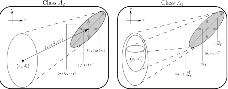
See the appendix for the explicit formulas and fig. 1 for an schematic description of the final states. From such com- binations it is obvious that we cannot solve for the initial state parameters given a final state as expected; this is because the parametric space dimension is reduced from 5 to 2. The channel belonging to A
1[see eq. (23) with e
2= α = b
2= 0 and eq. (30)] maps every initial state to a single one characterized by σ
f= N and d ⃗
f= (0, −c
1)
T, see fig. 2 for a schematic description.
According to our ans¨ atze [see equations (5) and 6)], we conclude that one-mode SGQC can only have the func- tional forms given in eq. (3) and eq. (5). This is the central result our work and can be stated as:
Theorem 1 (One-mode singular Gaussian channels). A one-mode Gaussian quantum channel is singular if and only if it has one of the following functional forms in the position space representation
1.
2πb3exp [ı(b
1x
fr
f+ b
3x
ir
f+ b
4x
ir
i+ c
1x
f+ c
2x
i) − a
1x
2f− a
2x
fx
i− a
3x
2i], 2. ∣β∣ √
e
1/πδ(αx
f− βx
i)
× exp [ − a
2x
fx
i− a
1x
2f− a
3x
2i+ı(b
2x
fr
i+ b
3r
fx
i+ b
1r
fx
f+ b
4r
ix
i+ c
1x
f+ c
2x
i)
−e
1r
f2− e
2r
fr
i−
e2 2ri2
4e1
], with e
2α = 0.
Corollary 1 (Singular classes). A one-mode singular Gaussian channel belongs to class A
1if and only if its position representation has the following form:
√
e
1/πδ(x
i) exp [ −a
1x
2f+ı(b
2x
fr
i+b
1r
fx
f+c
1x
f) −e
1r
f2].
Otherwise the channel belongs to class A
2.
Since channels on each class are connected each other by unitary conjugations [15], a consequence of the the- orem and the subsequent corollary is that the set of al- lowed forms must remain invariant under unitary conju- gations. To show this we must know the possible func- tional forms of Gaussian unitaries. They are given by following lemma for one mode
Lemma 1 (One-mode Gaussian unitaries). Gaussian unitaries can have only GF or the one given by eq. (6).
Proof. Recalling that for a unitary GQC, T must be sym- plectic (TΩT
T= Ω) and N = 0. However, an inspec- tion to eq. (18) lead us to note that N ≠ 0 unless e
1di- verges. Thus Gaussian unitaries cannot have the form J
I[see eq. (5)]. An inspection of matrices T and N of GQC with GF [see eq. (27)] and the ones for J
II[see equations (19) and (25)] lead us to note the following two observa- tions: (i) in both cases we have N = 0 for a
n= 0 ∀n;
(ii) the matrix T is symplectic for GF when b
2= b
3, and when αη = βγ for J
II. In particular the identity map has the last form. This completes the proof.
One can now compute the concatenations of the SGQCs with Gaussian unitaries. This can be done straightforward using the well known formulas for Gaus- sian integrals and the Fourier transform of the Dirac delta. Given that the calculation is elementary, and for sake of brevity, we present only the resulting forms of each concatenation. To show this compactly we intro- duce the following abbreviations: Singular channels be- longing to class A
2with form J
Iand with α = 0, e
2= 0 and α = e
2= 0, will be denoted as δ
αA2
, δ
eA22
and δ
α,eA 22
, re- spectively; singular channels belonging to the same class but with GF will be denoted as G
A2; channels belong- ing to class A
1will be denoted as δ
A1; finally Gaussian unitaries with GF will be denoted as G
Uand the ones with form J
IIas δ
U. Writing the concatenation of two channels in the position representation as
J
(f)(x
f, r
f; x
i, r
i) =
∫
R2dx
′dr
′J
(1)(x
f, r
f; x
′, r
′) J
(2)(x
′, r
′; x
i, r
i) , (31) the resulting functional forms for J
(f)are given in table I.
As expected, the table shows that the integral has only the forms stated by our theorem. Additionally it shows the cases when unitaries change the functional form of class A
2, while for class A
1J
(f)has always the unique form enunciated by the corollary.
J
(1)J
(2)J
(f)δ
Aα2
G
UG
A2G
Uδ
Aα2
δ
αA2
δ
Aα2
δ
Uδ
αA2
δ
Uδ
Aα2
δ
αA2
δ
Ae22
G
Uδ
eA2G
Uδ
Ae2 22
G
A2δ
Ae22
δ
Uδ
eA22
δ
Uδ
Ae22
δ
eA2G
U, δ
Aα,e2 22
δ
Aα,e22
δ
Aα,e22
G
UG
A2δ
U, δ
Aα,e22
δ
Aα,e22
δ
Aα,e22
δ
Uδ
Aα,e22
δ
U, G
Uδ
A1δ
A1δ
A1δ
U, G
Uδ
A1TABLE I. The first and second columns show the functional forms of J
(1)and J
(2), respectively. The last column shows the resulting form of the concatenation of them [see eq. (31)].
See main text for symbol coding.
V. EXISTENCE OF MASTER EQUATIONS
In this section we show the conditions under which master equations, associated with the channels derived in sec. III, exist. To be more precise, we study if the functional forms derived above parametrize channels be- longing to one-parameter differentiable families of GQCs.
As a first step, we let the coefficients of forms presented in equations (5) and (6) to depend on time. Later we de- rive the conditions under which they bring any quantum state ρ(x, r; t) to ρ(x, r; t + ) (with > 0 and t ∈ [0, ∞)) smoothly, while holding the specific functional form of the channel, i.e.
ρ(x, r; t + ) = ρ(x, r; t) + L
t[ρ(x, r; t)] + O(
2), (32) where both ρ(x, r; t) and ρ(x, r; t+) are propagated from t = 0 with channels either with the form J
Ior J
II, and L
tis a bounded superoperator in the state subspace. This is basically the problem of the existence of a master equa- tion
∂
tρ(x, r; t) = L
t[ρ(x, r; t)] , (33) for such functional forms. Thus the problem is reduced to prove the existence of the linear generator L
t, also known as Liouvillian.
To do this we use an ansatz proposed in Ref. [17] to
investigate the existence and derive the master equation
Class A 2
r p
(σf)11(s1) (σf)22(s1)
(σf)12(s1)
~di7→
~df(s2)
σi, ~di
FIG. 1. Schematic picture of the channels belonging to class A
2, acting on Wigner functions of Gaussian states. The ex- plicit dependence of the final state in terms of the combina- tions s
1and s
2are presented in the appendix. As well the formulas for s
idepending on the form of the channel. The pic- tured coordinate system corresponds to the position variable r and its conjugate momentum.
for GFs,
L = L
c(t) + (∂
x, ∂
r)X(t) ⎛
⎝
∂
x∂
r⎞
⎠ + (x, r)Y(t) ⎛
⎝
∂
x∂
r⎞
⎠
+ (x, r)Z(t) ⎛
⎝ x r
⎞
⎠ (34) where L
c(t) is a complex function and
X(t) = ⎛
⎝
X
xx(t) X
xr(t) X
rx(t) X
rr(t)
⎞
⎠
(35) is a complex matrix as well as Y(t) and Z(t), whose entries are defined in a similar way as in eq. (35). Note that X(t) and Z(t) can always be chosen symmetric, i.e.
X
xr= X
rsand Z
xr= Z
rx. Thus we must determine 11 time-dependent functions from eq. (34). This ansatz is also appropriate to study the functional forms introduced in this work, given that the left hand side of eq. (33) only involves quadratic polynomials in x, r, ∂/∂x and ∂/∂r, as in the GF case.
Notice that singular channels do not admit a master equation since its existence implies that channels with the functional form involved can be found arbitrarily close from the identity channel. This is not possible for sin- gular channels due to the continuity of the determinant of the matrix T. This fact can be also shown using the ansatz of eq. (34), one finds infinitely Liuville operators, thus the master equation is not well defined.
For the non-singular cases presented in equations (5) and (6), the condition for the existence of a master equa-
Class A 1
r p
1 2e1
2a1+ b 2 1 2e1
−2eb1 1
(0,−c1)T
σi, ~di
FIG. 2. Schematic picture of the channels belonging to class A
1, acting on Wigner functions of Gaussian states. Every channel of this class maps every initial quantum state, in par- ticular GSs characterized by (σ
i, d ⃗
i), to a Gaussian state that depends only on the channel parameters. We indicate in the figure the values of the corresponding components of the first and second moments of the final Gaussian state. The pictured coordinate system corresponds to the position variable r and its conjugate momentum.
tion is obtained as follows. (i) Substitute the ansatz of eq. (34) in the right hand side of the eq. (33). (ii) Define ρ(x, r; t) using eq. (2), given an initial condi- tion ρ(x, r; 0), for each functional form J
I,II. (iii) Take ρ
f(x
f, r
f) → ρ(x, r; t) and ρ
i(x
i, r
i) → ρ(x, r; 0). Fi- nally, (iv) compare both sides of eq. (33). Defining A(t) = α(t)/β (t) and B(t) = γ(t)/η(t), the conclusion is that for both J
Iand J
II, a master equations exist if
c(t) ∝ A(t) (36)
holds, where c(t) = c
1(t) + A(t)c
2(t). Additionally, for
the form J
Ithe solutions for the matrices X(t), Y(t)
and Z(t) are given by
X
xx= X
xr= Y
rx= Z
rr= 0, Y
xx=
A ˙ A , L
c= Y
rr=
˙ e
1e
1−
˙ e
2e
2, X
rr=
˙ e
14e
21−
˙ e
22e
1e
2, Y
xr= ı (
λ
1e ˙
2e
1e
2+ λ
2A ˙ e
2A −
λ
1e ˙
12e
21− λ ˙
2e
2) , Z
xx=
λ
212
⎛
⎝
˙ e
2e
1e
2−
˙ e
12e
21⎞
⎠ +
λ
1e
2⎛
⎝ λ
2A ˙
A − λ ˙
2⎞
⎠
+ 2λ
3A ˙ A − λ ˙
3, Z
xr= ı ⎛
⎝ A ˙ A
⎛
⎝ e
1λ
2e
2− λ
12
⎞
⎠ +
λ ˙
12 − λ ˙
2e
1e
2+ λ
22
⎛
⎝
˙ e
2e
2−
˙ e
1e
1⎞
⎠
⎞
⎠ , (37) where we have defined the following coefficients: λ
1= b
1+ Ab
3, λ
2= b
2+ Ab
4and λ
3= a
1+ Aa
2+ A
2a
3.
For the form J
IIthe solutions are the following L
c= X
xx= X
xr= X
rr= Z
rr= 0,
Y
rx= Y
xr= 0, Y
xx=
A ˙ A , Y
rr=
B ˙ B . Z
xx= a
2(t) A(t) + ˙ 2a
1(t) A(t) ˙
A(t) − A(t)
2−˙ a
3(t) − A(t) a ˙
2(t) − a ˙
1(t), Z
xr= ı ⎛
⎝ 1 2
λ ˙ − λ 2
⎛
⎝ A ˙ A +
B ˙ B
⎞
⎠
⎞
⎠ ,
(38)
where λ = b
1+ Ab
3+ B(b
2+ Ab
4).
VI. CONCLUSIONS
In this work we have critically reviewed the deceptively natural idea that Gaussian quantum channels always ad- mit a Gaussian functional form. To this end, we went beyond the pioneering characterization of Gaussian chan- nels with Gaussian form presented in Ref. [12] in two new directions. First we have shown that, starting from their most general definition as mapping Gaussian states into Gaussian states, a more general parametrization of the coordinate representation of the one-mode case exists, that admits non-Gaussian functional forms. Second, we were able to provide a black-box characterization of such new forms by imposing complete positivity (not consid- ered in Ref. [12]) and trace preserving conditions. While our parametrization connects with the analysis done by Holevo [16] in the particular cases where besides hav- ing a non-Gaussian form the channel is also singular, it also allows the study of Gaussian unitaries, thus pro- viding similar classification schemes. We completed the
classification of the new types of channels by deriving the form of the Liouvillian super operator that gener- ates their time evolution in the form of a master equa- tion. Surprisingly, Gaussian quantum channels without Gaussian form can be experimentally addressed by means of the celebrated Caldeira-Legget model for the quan- tum damped harmonic oscillator, where the new types of channels described here naturally appear in the sub- ohmic regime.
ACKNOWLEDGEMENTS
We acknowledge PAEP and RedTC for financial sup- port. Support by projects CONACyT 285754, UNAM- PAPIIT IG100518 is acknowledged. CP acknowledges support by PASPA program from DGAPA-UNAM. CAM and JDU acknowledge financial support from the German Academic Exchange Service (DAAD). We are thankful to the University of Vienna where part of this project was done.
Appendix A: Explicit formulas for class A
2The explicit formulas of the final states for channels of class A
2with the form presented in eq. (6) with e
2= 0 are
(σ
f)
11= 1 2e
1, (σ
f)
22= (
α β )
2
( b
232e
1+ 2a
3) + α β (2a
2+
b
1b
3e
1) + 2a
1+
b
212e
1+ s
1, (σ
f)
12= −
α β
b
32e
1− b
12e
1, d ⃗
f(s
3) = (0, −
α
β c
2− c
1+ s
2)
T
, (A1)
where
s
1= (b
22+ 2 α β b
2b
4+ (
α β )
2
b
24) (σ
i)
11− 2 ( α β b
2+ (
α β )
2
b
4) (σ
i)
12+ ( α β )
2
(σ
i)
22, s
2= (
α
β b
4+ b
2) (d
i)
1− α
β (d
i)
2. (A2)
The explicit formulas of the final states for channels of class A
2with the form presented in eq. (6) with α = 0 are
(σ
f)
11= e
224e
21(σ
i)
11+ 1 2e
1, (σ
f)
12= (
b
2e
22e
1− b
1e
224e
21) (σ
i)
11− b
12e
1, (σ
f)
22= 2a
1+ (b
2−
b
1e
22e
1)
2
(σ
i)
11+ b
212e
1, (A3)
and d ⃗
f= (
e
22e
1( ⃗ d
i)
1
, (b
2− b
1e
22e
1) ( ⃗ d
i)
1
− c
1)
T
. (A4) The explicit formulas of the final states for channels of class A
2with Gaussian form are
(σ
f)
11(s
1) = 2a
3b
23+ s
1, (σ
f)
12(s
1) =
a
2b
3− 2a
3b
1b
23− b
1s
1, (σ
f)
22(s
1) =
b
1(b
3(b
1b
3s
1− 2a
2) + 2a
3b
1) b
23+ 2a
1, d ⃗
f(s
2) = (s
2−
c
2b
3, b
1( c
2b
3− s
2) − c
1)
T