Detecting Pedestrians Using Patterns of Motion and Appearance

(1)

Detecting Pedestrians Using Patterns of Motion and Appearance

Paul Viola Michael J. Jones Daniel Snow

Microsoft Research Mitsubishi Electric Research Labs Mitsubishi Electric Research Labs

viola@microsoft.com mjones@merl.com snow@merl.com

Abstract

This paper describes a pedestrian detection system that in- tegrates image intensity information with motion informa- tion. We use a detection style algorithm that scans a detec- tor over two consecutive frames of a video sequence. The detector is trained (using AdaBoost) to take advantage of both motion and appearance information to detect a walk- ing person. Past approaches have built detectors based on motion information or detectors based on appearance in- formation, but ours is the first to combine both sources of information in a single detector. The implementation de- scribed runs at about 4 frames/second, detects pedestrians at very small scales (as small as 20x15 pixels), and has a very low false positive rate.

Our approach builds on the detection work of Viola and Jones. Novel contributions of this paper include: i) devel- opment of a representation of image motion which is ex- tremely efficient, and ii) implementation of a state of the art pedestrian detection system which operates on low res- olution images under difficult conditions (such as rain and snow).

1 Introduction

Pattern recognition approaches have achieved measurable success in the domain of visual detection. Examples include face, automobile, and pedestrian detection [14, 11, 13, 1, 9].

Each of these approaches use machine learning to construct a detector from a large number of training examples. The detector is then scanned over the entire input image in order to find a pattern of intensities which is consistent with the target object. Experiments show that these systems work very well for the detection of faces, but less well for pedestrians, perhaps because the images of pedestrians are more varied (due to changes in body pose and clothing). Detec- tion of pedestrians is made even more difficult in surveil- lance applications, where the resolution of the images is very low (e.g. there may only be 100-200 pixels on the target). Though improvement of pedestrian detection using better functions of image intensity is a valuable pursuit, we take a different approach.

This paper describes a pedestrian detection system that integrates intensity information with motion information.

The pattern of human motion is well known to be readily distinguishable from other sorts of motion. Many recent papers have used motion to recognize people and in some cases to detect them ([8, 10, 7, 3]). These approaches have a much different flavor from the face/pedestrian detection approaches mentioned above. They typically try to track moving objects over many frames and then analyze the motion to look for periodicity or other cues.

Detection style algorithms are fast, perform exhaustive search over the entire image at every scale, and are trained using large datasets to achieve high detection rates and very low false positive rates. In this paper we apply a detection style approach using information about motionas well asintensity information. The implementation described is very efficient, detects pedestrians at very small scales (as small as 20x15 pixels), and has a very low false positive rate. The system is trained on full human figures and does not currently detect occluded or partial human figures.

Our approach builds on the detection work of Viola and Jones [14]. Novel contributions of this paper include: i) development of a representation of image motion which is extremely efficient, and ii) implementation of a state of the art pedestrian detection system which operates on low resolution images under difficult conditions (such as rain and snow).

2 Related Work

The field of human motion analysis is quite broad and has a history stretching back to the work of Hoffman and Flinch- baugh [6]. Much of the field has presumed that the moving object has been detected, and that the remaining problem is to recognize, categorize, or analyze the long-term pattern of motion. Interest has recently increased because of the clear application of these methods to problems in surveil- lance. An excellent overview of related work in this area can be found in the influential paper by Cutler and Davis [3]. Cutler and Davis describe a system that is more direct than most, in that it works directly on images which can be of low resolution and poor quality. The system measures

(2)

periodicity robustly and directly from the tracked images.

Almost all other systems require complex intermediate representations, such as points on the tracked objects or the segmentation of legs. Detection failures for these interme- diates will lead to failure for the entire system.

In contrast our system works directly with images extracting short term patterns of motion, as well as appearance information, to detect all instances of potential objects.

There need not be separate mechanisms for tracking, segmentation, alignment, and registration which each involve parameters and adjustment. One need only select a feature set, a scale for the training data, and the scales used for detection. All remaining tuning and adjustment happens auto- matically during the training process.

Since our analysis is short term, the absolute false positive rate of our technique is unlikely to be as low as might be achieved by long-term motion analysis such as Cutler and Davis. Since the sources of motion are large, random processes may generate plausible “human” motion in the short term. In principle the two types of techniques are quite complimentary, in that hypothetical objects detected by our system could be verified using a long-term analysis.

The field of object detection is equally broad. To our knowledge there are no other systems which perform direct detection of pedestrians using both intensity and motion information. Key related work in the area use static intensity images as input. The system of Gavrila and Philomen [4]

detects pedestrians in static images by first extracting edges and then matching to a set of exemplars. This is a highly optimized and practical system, and it appears to have been a candidate for inclusion in Mercedes automobiles. Never- theless published detection rates were approximately 75%

with a false positive rate of 2 per image.

Other related work includes that of Papageorgiou et. al [9]. This system detects pedestrians using a support vector machine trained on an overcomplete wavelet basis. Because there is no widely available testing set, a direct comparison with our system is not possible. Based on the published experiments, the false positive rate of this system was signifi- cantly higher than for the related face detection systems. We conjecture that Papageorgiou et al.’s detection performance on static images would be very similar to our experiments on static images alone. In this case the false positive rate for pedestrian detection on static images is approximately 10 times higher than on motion pairs.

3 Detection of Motion Patterns

The dynamic pedestrian detector that we built is based on the simple rectangle filters presented by Viola and Jones [14] for the static face detection problem. We first extend these filters to act on motion pairs. The rectangle filters proposed by Viola and Jones can be evaluated extremely

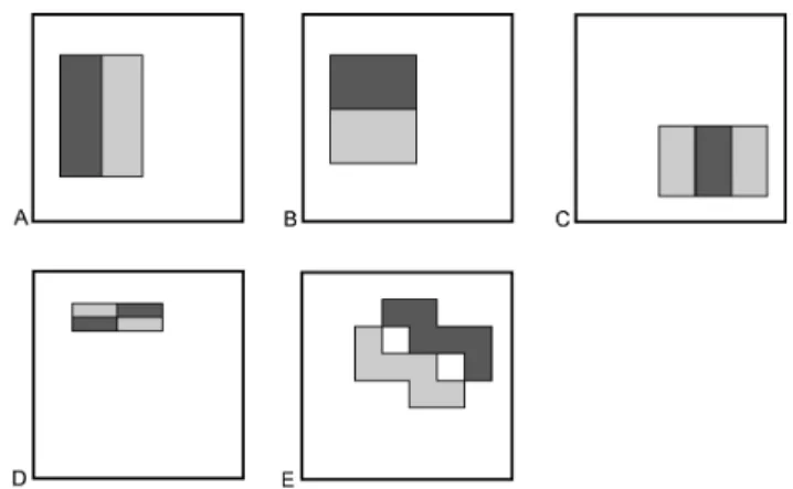
Figure 1: Example rectangle filters shown relative to the enclosing detection window. The sum of the pixels which lie within the lighter rectangles are subtracted from the sum of pixels in the darker rectangles. For three-rectangle filters the sum of pixels in the darker rectangle is multiplied by 2 to account for twice as many lighter pixels.

rapidly at any scale (see figure 1). They measure the differences between region averages at various scales, orienta- tions, and aspect ratios. While these features are somewhat limited, experiments demonstrate that they provide useful information that can be boosted to perform accurate classification.

Motion information can be extracted from pairs or sequences of images in various ways, including optical flow and block motion estimation. Block motion estimation requires the specification of a comparison window, which de- termines the scale of the estimate. This is not entirely com- patible with multi-scale object detection. In the context of object detection, optical flow estimation is typically quite expensive, requiring 100s or 1000s of operations per pixel.

Let us propose a natural generalization of the Viola- Jones features which operate on the differences between pairs of images in time. Clearly some information about motion can be extracted from these differences. For exam- pele, regions where the sum of the absolute values of the differences is large correspond to motion. Information about the direction of motion can be extracted from the difference between shifted versions of the second image in time with the first image.

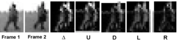
Motion filters operate on 5 images:

(3)

Figure 2: An example of the various shifted difference images used in our algorithm. The first two images are two typical frames with a low resolution pedestrian pictured.

The following images show the ,,,andimages described in the text. Notice that the right-shifted image difference () which corresponds to the direction of motion shown in the two frames has the lowest energy.

where and are images in time, andare image shift operators ( is shifted up by one pixel).

See Figure 2 for an example of these images.

One type of filter compares sums of absolute differences between and one ofU, L, R, D

where is one of and is a single box rectangular sum within the detection window. These filters extract information related to the likelihood that a particular region is moving in a given direction.

The second type of filter compares sums within the same motion image:

where is one of the rectangle filters shown in figure 1.

These features measure something closer to motion shear.

Finally, a third type of filter measures the magnitude of motion in one of the motion images:

where is one of andis a single box rectangular sum within the detection window.

We also use appearance filters which are simply rectangle filters that operate on the first input image, :

The motion filters as well as appearance filters can be evaluated rapidly using the “integral image” [14, 2] of

.

Because the filters shown in figure 1 can have any size, aspect ratio or position as long as they fit in the detection window, there are very many possible motion and appearance filters. The learning algorithm selects from this huge library of filters to build the best classifier for separating positive examples from negative examples.

A classifier,, is a thresholded sum of features:

if

otherwise

(1) A feature,, is simply a thresholded filter that outputs one of two votes.

if

otherwise (2)

where

is a feature threshold and is one of the motion or appearance filters defined above. The real-valued

and are computed during AdaBoost learning (as is the filter, filter thresholdand classifier threshold).

In order to support detection at multiple scales, the image shift operatorsmust be defined with respect to the detection scale. This ensures that measurements of motion velocity are made in a scale invariant way. Scale invariance is achieved during the training process simply by scaling the training images to a base resolution of 20 by 15 pixels. The scale invariance of the detection is achieved by operating on image pyramids. Initially the pyramids of and are computed. Pyramid representations of

are computed as follows:

whererefers to the the-th level of the pyramid. Classi- fiers (and features) which are learned on scaled 20x15 training images, operate on each level of the pyramid in a scale invariant fashion. In our experiments we used a scale factor of 0.8 to generate each successive layer of the pyramid and stopped when the image size was less than 20x15 pixels.

4 Training Process

The training process uses AdaBoost to select a subset of features and construct the classifier. In each round the learning algorithm chooses from a heterogenous set of filters, including the appearance filters, the motion direction filters, the motion shear filters, and the motion magnitude filters.

The AdaBoost algorithm also picks the optimal threshold for each feature as well as theandvotes of each feature.

The output of the AdaBoost learning algorithm is a classifier that consists of a linear combination of the selected features. For details on AdaBoost, the reader is referred to [12, 5]. The important aspect of the resulting classifier to

(4)

Figure 3: Cascade architecture. Input is passed to the first classifier with decides true or false (pedestrian or not pedestrian). A false determination halts further computation and causes the detector to return false. A true determination passes the input along to the next classifier in the cascade.

If all classifiers vote true then the input is classified as a true example. If any classifier votes false then computation halts and the input is classified as false. The cascade architecture is very efficient because the classifiers with the fewest features are placed at the beginning of the cascade, minimizing the total required computation.

note is that it mixes motion and appearance features. Each round of AdaBoost chooses from the total set of the various motion and appearance features, the feature with lowest weighted error on the training examples. The resulting classifier balances intensity and motion information in order to maximize detection rates.

Viola and Jones [14] showed that a single classifier for face detection would require too many features and thus be too slow for real time operation. They proposed a cascade architecture to make the detector extremely efficient (see figure 3). We use the same cascade idea for pedestrian detection. Each classifier in the cascade is trained to achieve very high detection rates, and modest false positive rates. Simpler detectors (with a small number of features) are placed earlier in the cascade, while complex detectors (with a large number of features are placed later in the cascade). Detection in the cascade proceeds from simple to complex.

Each stage of the cascade consists of a classifier trained by the AdaBoost algorithm on the true and false positives of the previous stage. Given the structure of the cascade, each stage acts to reduce both the false positive rate and the detection rate of the previous stage. The key is to reduce the false positive rate more rapidly than the detection rate.

A target is selected for the minimum reduction in false positive rate and the maximum allowable decrease in detection rate. Each stage is trained by adding features until the target detection and false positives rates are met on a validation set. Stages of the cascade are added until the overall target for false positive and detection rate is met.

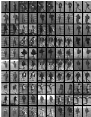
Figure 5: A small sample of positive training examples. A pair of image patterns comprise a single example for training.

5 Experiments

5.1 Dataset

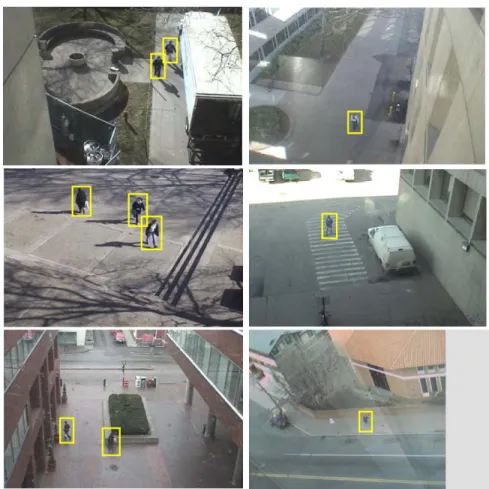
We created a set of video sequences of street scenes with all pedestrians marked with a box in each frame. We have eight such sequences, each containing around 2000 frames.

One frame of each sequence used for training along with the manually marked boxes is shown in figure 4.

5.1.1 Training Set

We used six of the sequences to create a training set from which we learned both a dynamic pedestrian detector and a static pedestrian detector. The other two sequences were used to test the detectors. The dynamic detector was trained on consecutive frame pairs and the static detector was trained on static patterns and so only uses the appearance filters described above. The static pedestrian detector uses the same basic architecture as the face detector described in [14].

Each stage of the cascade is a boosted classifier trained using a set of 2250 positive examples and 2250 negative examples. Each positive training example is a pair of 20 x 15 pedestrian images taken from two consecutive frames of a video sequence. Negative examples are similar image

(5)

Figure 4: Sample frames from each of the 6 sequences we used for training. The manually marked boxes over pedestrians are also shown.

pairs which do not contain pedestrians. Positive examples are shown in figure 5. During training, all example images are variance normalized to reduce contrast variations. The same variance normalization computation is performed during testing.

Each classifier in the cascade is trained using the original 2250 positive examples plus 2250 false positives from the previous stages of the cascade. The resulting classifier is added to the current cascade to construct a new cascade with a lower false positive rate. The detection threshold of the newly added classifier is adjusted so that the false negative rate is very low. The threshold is set using a validation set of image pairs.

Validation is performed using full images which contain marked postive examples. The validation set for these experiments contains 200 frame pairs. The threshold of the newly added classifier is set so that at least 99.5% of the pedestrians that were correctly detected after the last stage are still correctly detected while at least 10% of the false positives after the last stage are eliminated. If this target cannot be met then more features are added to the current

classifier.

The cascade training algorithm also requires a large set of image pairs to scan for false postives. These false positives form the negative training examples for the subsequent stages of the cascade. We use a set of 4600 full image pairs which do not contain pedestrians for this purpose. Since each full image contains about 50,000 patches of 20x15 pixels, the effective pool of negative patches is larger than 20 million.

The static pedestrian detector is trained in the same way on the same set of images. The only difference in the training process is the absence of motion information. Instead of image pairs, training examples consist of static image patches.

5.2 Training the Cascade

The dynamic pedestrian detector was trained using 54,624 filters which were uniformly subsampled from the much larger set of all filters that fit in a 20 x 15 pixel window.

The static detector was trained using 24,328 filters also

(6)

Figure 6: The first 5 filters learned for the dynamic pedestrian detector. The 6 images used in the motion and appearance representation are shown for each filter.

Figure 7: The first 5 filters learned for the static pedestrian detector.

uniformly subsampled from the total possible set. There are fewer filters in the static set because the various types of motion filters are not used.

The first 5 features learned for the dynamic detector are shown in figure 6. It is clear from these that the detector is taking advantage of the motion information in the examples. The first filter, for example, is looking for a difference in the motion near the left edge of the detection box com- pared to motion in the interior. This corresponds to the fact that our examples have the pedestrian roughly centered and so the motion is greatest in the interior of the detection box.

The second filter is acting on the first image of the input image pair. It corresponds to the fact that pedetrians tend to be in the middle of the detection box and stand out from the background. Four of the first 5 filters act on one of the motion images. This confirms the importance of using motion cues to detect pedestrians.

The first 5 features learned for the static detector are shown in figure 7. The first filter is similar to the second filter learned in the dynamic case. The second filter is similar but focuses on the legs. The third filter focuses on the torso.

0 1 2 3 4 5 6 7 8

x 10⁻⁵ 0.2

0.3 0.4 0.5 0.6 0.7 0.8 0.9 1

False positive rate

Detection rate

ROC curve for pedestrian detection on test sequence 1

dynamic detector static detector

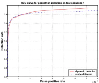
Figure 8: ROC curve on test sequence 1 for both the dynamic and static pedestrian detectors. Both detectors achieve a detection rate of about 80% with a false positive rate of about 1/400,000 (which corresponds to about 1 false positive every 2 frames for the 360x240 pixel frames of this sequence).

5.3 Detection Results

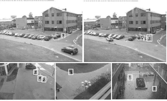
Some example detections for the dynamic detector are shown in figure 10. The detected boxes are displayed on the first frame of each image pair. Example detections for the static case are shown in figure 11. It is clear from these examples that the static detector usually has many more false positives than the dynamic detector. The top row of examples are taken from the PETS 2001 dataset. The PETS sequences were acquired independently using a different camera and a different viewpoint from our training sequences.

The detector seems to generalize to these new sequences quite well. The bottom row shows test performed using our own test data. The left two image sequences were not used during training. The bottom right image is a frame from the same camera and location used during training, though at a different time. This image shows that the dynamic detector works well under difficult conditions such as rain and snow, though these conditions did not occur in the training data.

We also ran both the static and dynamic detectors over test sequences for which ground truth is available. From these experiments the false positive rate (the number of false positives across all the frames divided by the total number of patches tested in all frames) and a false negative rate (the total number of false negatives in all frames divided by the total number of faces in all frames) were estimated.

Computation of a full ROC curve is not a simple mat- ter, since the false positive and negative rates depend on the threshold chosen for all layers of the cascade. By adjust-

(7)

0 1 2 3 4 5 6 x 10⁻⁵ 0.2

0.3 0.4 0.5 0.6 0.7 0.8 0.9 1

False positive rate

Detection rate

ROC curve for pedestrian detection on test sequence 2

dynamic detector static detector

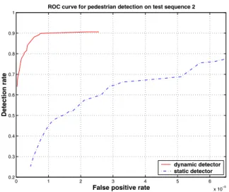
Figure 9: ROC curve on test sequence 2 for both the dynamic and static pedestrian detectors. The dynamic detector has much greater accuracy in this case. At a detection rate of 80%, the dynamic detector has a false positive rate of about 1/400,000 while the static detector has a false positive rate of about 1/15,000.

ing these thresholds one at a time we get a ROC curve for both the dynamic and static detectors. These ROC curves are shown in figures 8 and 9. The ROC curve for the dynamic case is an order of magnitude better on sequence 2 than the static case. On sequence 1, the dynamic detector is only slightly better than the static one. This is probably due to the fact that sequence 2 has some highly textured areas such as the tree and grass that are more likely to cause false positives in the static case.

6 Conclusions

We have presented a detection style algorithm which combines motion and appearance information to build a robust model of walking humans. This is the first approach that we are aware of that combines both motion and appearance in a single model. Our system robustly detects pedestrians from a variety of viewpoints with a low false positive rate.

The basis of the model is an extension of the rectangle filters from Viola and Jones to the motion domain. The advantage of these simple filters is their extremely low computation time. As a result, the pedestrian detector is very efficient. It takes about 0.25 seconds to detect all pedestrians in a 360 x 240 pixel image on a 2.8 GHz P4 processor.

About 0.1 seconds of that time is spent actually scanning the cascade over all positions and scales of the image and 0.15 seconds are spent creating the pyramids of difference images. Using optimized image processing routines we be-

lieve this can be further improved.

The idea of building efficient detectors that combine both motion and appearance cues will be applicable to other problems as well. Candidates include other types of human motion (running, jumping), facial expression classification, and possible lip reading.

References

[1] S. Avidan. Support vector tracking. InIEEE Conference on Computer Vision and Pattern Recognition, 2001.

[2] F. Crow. Summed-area tables for texture mapping. In Proceedings of SIGGRAPH, volume 18(3), pages 207–212, 1984.

[3] R. Cutler and L. Davis. Robust real-time periodic motion detection: Analysis and applications. InIEEE Patt. Anal.

Mach. Intell., volume 22, pages 781–796, 2000.

[4] V. Philomin D. Gavrila. Real-time object detection for

”smart” vehicles. InIEEE International Conference on Com- puter Vision, pages 87–93, 1999.

[5] Yoav Freund and Robert E. Schapire. A decision-theoretic generalization of on-line learning and an application to boosting. InComputational Learning Theory: Eurocolt ’95, pages 23–37. Springer-Verlag, 1995.

[6] D. D. Hoffman and B. E. Flinchbaugh. The interpretation of biological motion. Biological Cybernetics, pages 195–204, 1982.

[7] L. Lee. Gait dynamics for recognition and classification. Mit ai lab memo aim-2001-019, MIT, 2001.

[8] F. Liu and R. Picard. Finding periodicity in space and time. InIEEE International Conference on Computer Vision, pages 376–383, 1998.

[9] C. Papageorgiou, M. Oren, and T. Poggio. A general frame- work for object detection. InInternational Conference on Computer Vision, 1998.

[10] R. Polana and R. Nelson. Detecting activities.Journal of Vi- sual Communication and Image Representation, June 1994.

[11] H. Rowley, S. Baluja, and T. Kanade. Neural network-based face detection. InIEEE Patt. Anal. Mach. Intell., volume 20, pages 22–38, 1998.

[12] R. Schapire and Y. Singer. Improving boosting algorithms using confidence-rated predictions, 1999.

[13] H. Schneiderman and T. Kanade. A statistical method for 3D object detection applied to faces and cars. InInternational Conference on Computer Vision, 2000.

[14] P. Viola and M. Jones. Rapid object detection using a boosted cascade of simple features. InIEEE Conference on Com- puter Vision and Pattern Recognition, 2001.

(8)

Figure 10: Example detections for the dynamic detector. Note the rain and snow falling in the image on the lower right.

Figure 11: Example detections for the static detector.