Numerical Methods for Non-local Operators

Numerical Methods for Non-local Operators

Steffen B¨ orm

1:17, February 4, 2021

All rights reserved.

Contents

1 Introduction 5

2 One-dimensional model problem 9

2.1 Integral equation and discretization . . . . 9

2.2 Degenerate approximation . . . . 11

2.3 Error analysis . . . . 12

2.4 Hierarchical partition . . . . 15

2.5 Complexity . . . . 17

2.6 Approximation by interpolation . . . . 21

2.7 Interpolation error analysis . . . . 24

2.8 Improved interpolation error estimates . . . . 28

3 Multi-dimensional problems 37 3.1 Gravitational potentials . . . . 37

3.2 Approximation by interpolation . . . . 38

3.3 Error analysis . . . . 41

3.4 Cluster tree and block tree . . . . 47

3.5 Hierarchical matrices . . . . 53

3.6 Complexity estimates . . . . 54

3.7 Estimates for cluster trees and block trees . . . . 60

3.8 Improved interpolation error estimates . . . . 66

4 Low-rank matrices 73 4.1 Definition and basic properties . . . . 73

4.2 Low-rank approximation . . . . 78

4.3 Rank-revealing QR factorization . . . . 91

4.4 Rank-revealing LR factorization and cross approximation . . . . 93

4.5 Hybrid cross approximation . . . . 100

4.6 Global norm estimates . . . . 102

5 Arithmetic operations 107 5.1 Matrix-vector multiplication . . . . 107

5.2 Complexity of the matrix-vector multiplication . . . . 109

5.3 Truncation . . . . 113

5.4 Low-rank updates . . . . 115

5.5 Merging . . . . 118

5.6 Matrix multiplication . . . . 122

5.7 Complexity of the matrix multiplication . . . . 126

5.8 Inversion . . . . 133

5.9 Triangular factorizations . . . . 139

6 H

-matrices 155 6.1 Motivation . . . . 155

6.2 H

-matrices . . . . 159

6.3 Matrix-vector multiplication . . . . 163

6.4 Low-rank structure of H

-matrices . . . . 167

7 H

-matrix compression 173 7.1 Orthogonal projections . . . . 173

7.2 Adaptive cluster bases . . . . 176

7.3 Compression error . . . . 182

7.4 Compression of H-matrices . . . . 187

7.5 Compression of H

-matrices . . . . 190

Index 203

1 Introduction

Non-local operators appear naturally in a wide range of applications, e.g., in the inves- tigation of gravitational, electromagnetic or acoustic fields. Handling non-local interac- tions poses an interesting algorithmic challenge: we consider classical gravitational fields as an example. In a first step, we consider two stars located at positions x, x ˆ ∈ R

with masses m, m ˆ ∈ R

. The gravitational force exerted by the star at position x on the star at position ˆ x is given by

f ˆ = γ mm ˆ x − x ˆ kx − xk ˆ

where γ ∈ R

is the universal gravitational constant. If we consider only two interacting stars, we can evaluate this expression directly and efficiently and use it as the basis of simulations.

The situation changes significantly if we consider a larger number of stars: Let n ∈ N , and let x

, . . . , x

∈ R

be positions and m

, . . . , m

∈ R

masses of n different stars.

By the superposition principle, the gravitational forces exerted on a star at position ˆ x result from adding the individual forces, i.e., we have

f ˆ = γ m ˆ

n

X

j=1

m

x

− x ˆ kx

− xk ˆ

.

Now the evaluation of the force requires Θ(n) operations. Since even a small galaxy contains around 10

and the Milky Way is estimated to contain between 2 × 10

and 4 × 10

stars, evaluating ˆ f takes a long time. If we wanted to simulate the motion of all stars in the Milky Way, we would have to evaluate the forces exerted on each star by all other stars, leading to at least 2 × 10

operations. This is an amount of computational work that even modern parallel computers cannot handle: a single core of a processor might be able to compute 10

forces per second, so it would take at least 2×10

seconds, i.e., approximately 633 761 years. Even if we could parallelize the evaluation perfectly and had 633 761 processor cores at our disposal, one evaluation of the forces would still take a year, and standard time-stepping methods require a large number of evaluations to obtain a reasonably accurate simulation.

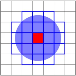
We can work around this problem by employing an approximation: let s ⊆ R

be a convex subdomain, and let

ˆ

s := {j ∈ I : x

∈ s}, I := [1 : n]

denote the indices of all stars located in s.

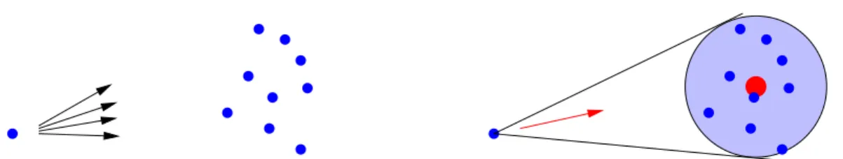
Figure 1.1: Replacing a cluster of stars by a “virtual star” that exerts approximately the same gravitational force

If the diameter of s is small compared to the distance from s to ˆ x, we have x

− x ˆ

kx

− xk ˆ

≈ x

− x ˆ

kx

− xk ˆ

for all j ∈ ˆ s,

where x

denotes the (suitably defined) center of s. Using this approximation, we obtain X

j∈ˆs

m

x

− x ˆ

kx

− xk ˆ

≈ X

j∈ˆs

m

x

− x ˆ kx

− xk ˆ

=



 X

j∈ˆs

m





| {z }

=:ms

x

− x ˆ

kx

− xk ˆ

= m

x

− x ˆ kx

− xk ˆ

.

If we have x

and m

at our disposal, evaluating this expression requires only O(1) operations. Essentially we approximate all stars in the region s by a single “virtual”

star at position x

of mass m

. Considering that s may contain millions or even billions of stars, replacing them by a single one significantly reduces the computational work.

In most cases, a single subdomain s cannot contain all stars and at the same time be sufficiently far from ˆ x. This problem can be solved by using a nested hierarchy of subdomains: given a subdomain s containing a number of stars, we check whether it is sufficiently far from ˆ x. If it is, we use our approximation. Otherwise, we split s into sub- domains and check these subdomains recursively. We can arrange the splitting algorithm in a way that guarantees that the diameters of the subdomains decay exponentially, and prove that O(log n) subdomains are sufficient to approximate the force acting at ˆ x.

This approach can be generalized and made more efficient, e.g., we can improve the

accuracy by using multiple virtual stars per subdomain s, we can reduce the computa-

tional work by constructing virtual stars for s from virtual stars of subdomains s

instead

of the original stars. The best methods employ hierarchies of source subdomains s and

target subdomains t that are both represented by virtual stars: in a first step, the stars

in the source subdomains are replaced by virtual stars. In a second step, the interactions

between virtual source stars in s and virtual target stars in t are computed. In a final

step, the forces acting on the virtual target stars in t are translated back to forces acting

on real target stars. This technique can reach almost linear complexity and is known as

a fast multipole method [22] or as a symmetric panel clustering method [30]. Its algebraic

counterpart is the H

-matrix representation [27, 8].

A particularly interesting application is the approximation of matrices resulting from the discretization of integral equations or partial differential equations: instead of using k virtual stars to approximate a gravitational field, we use k coefficients to approximate the effect of a submatrix. Considered from an algebraic point of view, this is equivalent to approximating a submatrix by a matrix of rank k, and this kind of approximation can be constructed efficiently for matrices appearing in a large number of practical applications.

Splitting a matrix hierarchically into submatrices that can be approximated by low rank leads to the concept of hierarchical matrices (or short H-matrices) [23, 26, 25, 21, 24]. These matrices are of particular interest, since they can be used to replace fully populated matrices in a wide range of applications using specialized algorithms for handling matrix products, inverses, or factorizations. This approach leads to very efficient and robust preconditioners for integral equations and elliptic partial differential equations, it can be used to evaluate matrix functions or to solve certain kinds of matrix equations.

Taking the concept of low-rank approximations a step further leads to H

-matrices [27, 8, 6] that handle multiple low-rank blocks simultaneously in order to reduce storage requirements and computational work even further.

Acknowledgements

I would like to thank Daniel Hans, Christina B¨ orst, Jens Liebenau, Jonathan Schilling,

Jan-Niclas Thiel, Bennet Carstensen, Jonas Lorenzen, Nils Kr¨ utgen, and Nico Wichmann

for helpful corrections.

2 One-dimensional model problem

We start with a one-dimensional model problem that shares many important properties with “real” applications, but is sufficiently simple to allow us to analyze both accuracy and complexity without the need for elaborate new tools

2.1 Integral equation and discretization

We consider the integral equation Z

0

g(x, y)u(y) dy = f(x) for all x ∈ [0, 1], (2.1) where the kernel function g is given by

g(x, y) :=

( − log |x − y| if x 6= y,

0 otherwise for all x, y ∈ [0, 1] (2.2)

and the right-hand side f and the solution u are in a suitable function spaces. Here log(z) denotes the natural logarithm of z ∈ R

, i.e., we have log(e

) = z.

In order to compute an approximation of the solution u, we consider a variational formulation: we choose a subspace V of L

[0, 1] for both the solution u and the right- hand side f and multiply (2.1) by test functions v ∈ V to obtain the following problem:

Find u ∈ V such that Z

0

v(x) Z

0

g(x, y)u(y) dy dx = Z

0

v(x)f (x) dx for all v ∈ V .

We will not investigate the appropriate choice of the space V here, although it is of course important for the existence and uniqueness of solutions.

We are only interested in the Galerkin discretization of the variational formulation:

we let n ∈ N and introduce piecewise constant basis functions ϕ

(x) :=

( 1 if x ∈ [(i − 1)/n, i/n]

0 otherwise for all i ∈ [1 : n], x ∈ [0, 1].

Following the standard Galerkin approach, the space V is replaced by V

:= span{ϕ

: i ∈ [1 : n]}

to obtain the following finite-dimensional variational problem:

Find u

∈ V

such that Z

0

v

(x) Z

0

g(x, y)u

(y) dy dx = Z

0

v

(x)f(x) dx for all v

∈ V

.

In order to compute u

, we express it in terms of the coefficient vector z ∈ R

corre- sponding to our basis, i.e., we have

u

=

n

X

j=1

z

ϕ

. Testing with basis vectors yields

n

X

j=1

z

Z

ϕ

(x) Z

0

g(x, y)ϕ

(y) dy dx = Z

0

ϕ

(x)f (x) dx for all i ∈ [1 : n], and this describes an n-dimensional linear system of equations.

Introducing the matrix G ∈ R

and the vector b ∈ R

by g

:=

Z

ϕ

(x) Z

0

g(x, y)ϕ

(y) dy dx for all i, j ∈ [1 : n], (2.3a) b

:=

Z

ϕ

(x)f (x) dx for all i ∈ [1 : n], (2.3b)

we can write this linear system in the compact form

Gz = b. (2.4)

Since G is an n-dimensional square matrix, we have to store n

coefficients. In order to make u

a reasonably accurate approximation of u, we typically have to choose n relatively large, so that storing n

coefficients is unattractive.

Since g(x, y) > 0 holds for almost all x, y ∈ [0, 1], all coefficients are non-zero, so standard data structures like sparse matrices or band matrices cannot be applied.

Remark 2.1 (Toeplitz matrix) G is a Toeplitz matrix, i.e., we have j − i = ` − k = ⇒ a

= a

for all i, j, k, ` ∈ [1 : n].

Toeplitz matrices can be embedded in circulant matrices, and circulant matrices can be diagonalized using the discrete Fourier transformation.

This means that we can use the fast Fourier transformation algorithm [10] to evalu- ate matrix-vector products in O(n log n) operations. Unfortunately, this approach relies heavily on the regular structure of our discretization and is typically not an option for more general problems.

Remark 2.2 (Wavelets) Another approach is to use wavelet basis functions [13, 9]

instead of piecewise constant functions.

This reduces the absolute value of most matrix elements significantly and thereby al-

lows us to approximate the entire matrix G by a sparse matrix that can be handled very

efficiently. This approach can be extended to more general geometries and integral opera-

tors [12, 14, 11], but the corresponding algorithm is more complicated than the technique

we will focus on here.

2.2 Degenerate approximation

2.2 Degenerate approximation

We are looking for a data-sparse approximation of the matrix G, i.e., a representation that requires us to store only a relatively small number of coefficients. In the case of the integral equation (2.1), we can take advantage of the fact that the kernel function g is analytic as long as we stay away from the singularity at x = y: if we have two intervals t = [a, b] and s = [c, d] with t ∩ s = ∅, the restriction g|

of g to the axis-parallel box t × s = [a, b] × [c, d] is an analytic function and can be approximated by polynomials.

For the sake of simplicity, we consider a straightforward Taylor expansion of the func- tion x 7→ g(x, y) for a fixed y ∈ s. For an order m ∈ N , the Taylor polynomial centered at x

∈ t is given by

˜

g

(x, y) :=

m−1

X

ν=0

(x − x

)

ν!

∂

g

∂x

(x

, y) for all x ∈ t, y ∈ s. (2.5) This is an example of a degenerate approximation, i.e., it is a sum of tensor products

˜

g

(x, y) =

m−1

X

ν=0

a

(x)b

(y) for all x ∈ t, y ∈ s (2.6) with

a

(x) := (x − x

)

ν! , b

(y) := ∂

g

∂x

(x

, y) for all ν ∈ [0 : m], x ∈ t, y ∈ s.

Degenerate approximations are useful because they immediately lead to data-sparse approximations: if we assume ˜ g

≈ g|

, we find

g

= Z

0

ϕ

(x) Z

0

g(x, y)ϕ

(y) dy dx = Z

(i−1)/n

Z

g(x, y) dy dx

≈ Z

(i−1)/n

Z

˜

g

(x, y) dy dx =

m−1

X

ν=0

Z

a

(x) dx Z

(j−1)/n

b

(y) dy for all i, j ∈ [1 : n] with

supp ϕ

= [(i − 1)/n, i/n] ⊆ t, supp ϕ

= [(j − 1)/n, j/n] ⊆ s. (2.7) We collect the indices of all row basis functions satisfying the first condition in a set

ˆ t := {i ∈ [1 : n] : supp ϕ

⊆ t},

and the indices of all column basis functions satisfying the second condition in ˆ

s := {j ∈ [1 : n] : supp ϕ

⊆ s},

therefore we should be able to replace g by ˜ g

in the integral (2.3a) for all row indices

i ∈ ˆ t and all column indices j ∈ ˆ s.

We obtain the approximation g

≈

m−1

X

ν=0

a

b

for all i ∈ ˆ t, j ∈ ˆ s

with the matrices matrices A

∈ R

, B

∈ R

, M := [0 : m − 1] given by a

:=

Z

ϕ

(x)a

(x) dx = Z

(i−1)/n

a

(x) dx for all i ∈ ˆ t, ν ∈ M, b

:=

Z

ϕ

(y)b

(y) dy = Z

(j−1)/n

b

(y) dy for all j ∈ ˆ s, ν ∈ M.

It is usually more convenient to write this approximation in the short form

G|

≈ A

B

, (2.8)

where B

denotes the adjoint (in this case the transposed) matrix of B

. If we store the factors A

and B

instead of G|

, we only require m(| ˆ t| + |ˆ s|) coefficients instead of

| ˆ t × ˆ s| = | t| |ˆ ˆ s|. If m is small, the factorized approximation can therefore be significantly more efficient than the original submatrix.

The range of the approximation A

B

is contained in the range of A

and therefore at most m-dimensional, therefore the approximation has at most a rank of m. Factorized low-rank approximations of this kind are a very versatile tool for dealing with non-local operators and play a crucial role in this book.

2.3 Error analysis

Since we are using an approximation of the kernel function g, we have to investigate the corresponding approximation error.

Reminder 2.3 (Taylor expansion) Let z

, z ∈ [a, b], and let f ∈ C

[a, b]. We have f(z) =

m−1

X

ν=0

(z − z

)

ν!

∂

f

∂z

(z

) + Z

0

(1 − τ )

(m − 1)!

∂

f

∂z

(z

+ τ (z − z

)) dτ (z − z

)

. Proof. Induction. The base case m = 1 is the fundamental theorem of calculus. The induction step is partial integration.

In the case of our approximation of the kernel function g, the statement of Re- minder 2.3 takes the form

g(x, y) − ˜ g

(x, y) = Z

0

(1 − τ )

(m − 1)!

∂

g

∂x

(x

+ τ (x − x

), y) dτ (x − x

)

.

In order to obtain a useful error estimate, we require the derivatives of g. These are

easily obtained, at least for our model problem.

2.3 Error analysis

xt

a b

c d

xt

a b c d

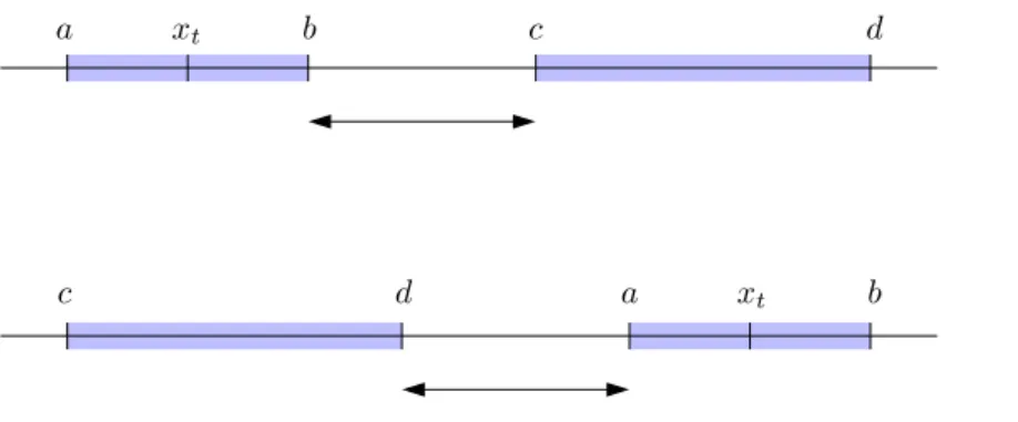
Figure 2.1: Distances and diameters of intervals Lemma 2.4 Let x, y ∈ R with x 6= y. We have

∂

g

∂x

(x, y) = (−1)

(m − 1)! (x − y)

,

∂

g

∂y

(x, y) = (m − 1)! (x − y)

for all m ∈ N.

Proof. Straightforward induction.

Since the kernel function g has singularities for x = y, the same holds for its derivatives, therefore the chances of bounding the error if the target interval t and the source interval s intersect are looking quite bleak. If we assume that t and s are disjoint, on the other hand, we can not only obtain error bounds, but these bounds even converge exponentially to zero as the order m increases.

Theorem 2.5 (Error estimate) Let x

= (b + a)/2 denote the midpoint of t = [a, b], let diam(t) = b − a denote its diameter and dist(t, s) = max{c − b, a − d, 0} the distance between t and s.

If dist(t, s) > 0, we have

|g(x, y) − g ˜

(x, y)| ≤ log(1 + η) η

η + 1

for all x ∈ t, y ∈ s with the admissibility parameter

η := diam(t)

2 dist(t, s) . (2.9)

Proof. Let dist(t, s) > 0, and let x ∈ t, y ∈ s. The triangle inequality and the equations for the derivatives provided by Lemma 2.4 yield

|g(x, y) − g ˜

(x, y)| ≤ Z

0

(1 − τ )

(m − 1)!

∂

g

∂x

(x

+ τ (x − x

), y)

dτ|x − x

|

= Z

0

(1 − τ )

(m − 1)!

(m − 1)!|x − x

|

|x

+ τ (x − x

) − y|

dτ

≤ Z

0

(1 − τ )

|x − x

| (|x

− y| − τ |x − x

|)

dτ. (2.10)

Due to dist(t, s) > 0, we have either c > b or a > d. In the first case (top in Figure 2.1), we have x, x

≤ b < c ≤ y. In the second case (bottom in Figure 2.1), we have y ≤ d <

a ≤ x, x

. This implies x

− y < 0 if c > b and x

− y > 0 if a > d, so we find

|x

− y| =

( y − x

= y − b + b − x

≥ c − b +

if c > b, x

− y = x

− a + a − y ≥

+ a − d if a > d,

and conclude |x

− y| ≥ diam(t)/2 + dist(t, s). Due to |x − x

| ≤ diam(t)/2, we obtain

|x − x

|

|x

− y| − τ |x − x

| ≤ diam(t)/2

dist(t, s) + (1 − τ ) diam(t)/2 . If diam(t) = 0 holds, the proof is complete.

Assuming now diam(t) > 0, we can introduce ζ := 1/η = 2 dist(t, s)

diam(t) , and write our estimate as

|x − x

|

|x

− y| − τ |x − x

| ≤ 1

2 dist(t, s)/ diam(t) + 1 − τ = 1 ζ + 1 − τ . The error estimate (2.10) takes the form

|g(x, y) − g ˜

(x, y)| ≤ Z

0

(1 − τ )

(ζ + 1 − τ )

dτ =

Z

σ

(ζ + σ)

dσ.

Due to

σ

ζ + σ ≤ 1

ζ + 1 for all σ ∈ [0, 1],

we arrive at

|g(x, y) − g ˜

(x, y)| ≤ 1

ζ + 1

Z

1

ζ + σ dσ = 1

ζ + 1

(log(ζ + 1) − log(ζ))

=

1/ζ 1 + 1/ζ

log(1 + 1/ζ ) = η

1 + η

log(1 + η).

This is the estimate we need.

If dist(t, s) > 0, we have

η = diam(t) 2 dist(t, s) < ∞

and the Taylor expansion ˜ g

(x, y) converges exponentially at a rate of η

η + 1 < 1

to g(x, y) for all x ∈ t and y ∈ s.

2.4 Hierarchical partition

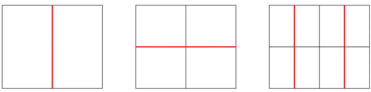
Figure 2.2: Simple cluster tree constructed by recursive bisection of the interval [0, 1]

2.4 Hierarchical partition

We can expect convergence only if we apply the approximation ˜ g

to subdomains t × s satisfying dist(t, s) > 0. In order to guarantee a certain rate of convergence, we have to ensure that the parameter η introduced in (2.9) is bounded.

Our approach is to “reverse” the roles of subdomain and admissibility parameter:

instead of choosing the paramter to fit the subdomains, we choose the subdomain to fit the parameter.

We fix η ∈ R

and check whether a given subdomain t × s satisfies the admissibility condition

diam(t) ≤ 2η dist(t, s). (2.11)

If it does, we can approximate the kernel function and obtain a factorized low-rank approximation. Otherwise, we split the subdomain, unless it is so small that we can afford storing the corresponding matrix directly.

In this example we use the choice η = 1/2, i.e., we consider a subdomain t×s admissible if diam(t) ≤ dist(t, s) holds. By Theorem 2.5, this leads to the error bound

|g(x, y) − g ˜

(x, y)| ≤ 3 log(3/2) 3

for all x ∈ t, y ∈ s, m ∈ N .

In general, the parameter η allows us to balance the rate of convergence against the number of subdomains, i.e., accuracy against computational work and storage.

For inadmissible subdomains, we use a simple splitting strategy based on bisection:

assume that t = [a, b] and s = [c, d] are inadmissible, i.e., that the condition (2.11) does not hold. We let

a

:= a, b

= a

:= b + a

2 , b

:= b,

c

:= c, d

= c

:= d + c

2 , d

:= d

and define

t

:= [a

, b

], t

:= [a

, b

], s

:= [c

, d

], s

:= [c

, d

],

i.e., we split t into two equal halves t

, t

, and s into two equal halves s

, s

.

Figure 2.3: Hierarchical subdivision of the domain [0, 1] × [0, 1]

Now we check whether the Cartesian products t

× s

, t

× s

, t

× s

, and t

× s

are admissible and proceed by recursion if they are not.

Our construction leads to a subdivision of [0, 1] into subintervals of the form t

:= [(α − 1)2

, α2

] for all ` ∈ N

, α ∈ [1 : 2

].

Each interval t

is split into

t

= [(α − 1)2

, (α − 1/2)2

] and t

= [(α − 1/2)2

, α2

].

We call these subintervals the sons of t

and arrive at a tree structure, cf. Figure 2.2, describing the subdivision of [0, 1] = t

. The Cartesian product [0, 1] × [0, 1] is split into Cartesian products t × s of pairs of elements of this tree.

Since we only split the domain, there are always subdomains t × s that include the diagonal {(x, y) ∈ [0, 1] × [0, 1] : x = y} and therefore do not satisfy the admissibility condition (2.11). In order to handle these subdomains, we stop splitting at a given maximal depth p ∈ N

of the recursion and store the remaining matrix entries directly.

The resulting decomposition of [0, 1]×[0, 1] into admissible and inadmissible subdomains can be seen in Figure 2.3.

The next step is to construct the approximation of the matrix G, i.e., to integrate the

products of basis functions and approximated kernel functions. In order to keep this task

as simple as possible, we assume that n = 2

holds with q ∈ N

, q ≥ p. This property

guarantees that the support [(i − 1)/n, i/n] of a basis function ϕ

is either completely

2.5 Complexity contained in one of our subintervals t or that the intersection is a null set, so that the integral vanishes.

Under these conditions, we have ˆ t

= [(α − 1)2

+ 1 : α2

], t

= [

{supp ϕ

: i ∈ ˆ t

} for all ` ∈ [0 : p], α ∈ [1 : 2

].

Storing the submatrices G|

for inadmissible domains t × s on level ` = p requires

| ˆ t| |ˆ s| = 4

coefficients, since | ˆ t| = |ˆ s| = 2

. As long as q is not significantly larger than p, this amount of storage is acceptable.

For admissible domains t × s on level `, we use the approximation (2.8) and store

| ˆ t| m = 2

m coefficients for the matrix A

and |ˆ s| m = 2

m coefficients for the matrix B

.

Remark 2.6 (Rank) If we replace g by g ˜

, we obtain an approximation G e ∈ R

of the matrix G. Solving G e x e = b instead of Gx = b leads to an error of

kx − xk e

kxk ≤ κ(G) 1 − κ(G)

kG − Gk e kGk .

In typical situations, we expect the condition number κ(G) to grow like n

for a constant c > 0, while the discretization error converges like n

for a constant d > 0.

In order to ensure that our approximation of the matrix adds only an additional error on the same order as the discretization error, we need the relative matrix error

to converge like n

. Due to our admissibility condition and Theorem 2.5, an order of m ∼ log(n) is sufficient to guarantee this property.

2.5 Complexity

Let us now consider the storage requirements of our approximation of the matrix G.

If t × s is admissible, we store the matrices A

and B

, and we have already seen that this requires m(| ˆ t| + |ˆ s|) coefficients. If t × s is not admissible, we store G|

in the standard way, and this requires 4

coefficients. In order to obtain an estimate for the approximation of the entire matrix, we have to know how many admissible and inadmissible domains appear in our decomposition of the domain [0, 1] × [0, 1].

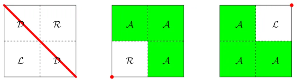
In our model situation, the construction of the domains is very regular and all domains t × s fall into one of the following for categories: we call t × s

• diagonal if t = s,

• right-neighbouring if max t = min s,

• left-neighbouring if min t = max s, and

• admissible otherwise.

R

L D

D

A

A A

R

L

A A

A

Figure 2.4: Diagonal, right-neighbouring, and left-neighbouring inadmissible domains with corresponding splitting patterns

By our construction, cf. Figure 2.4, a diagonal subdomain t ×s is split into two diagonal subdomains t

× s

and t

× s

, one right-neighbouring subdomain t

× s

and one left-neighbouring subdomain t

× s

.

A right-neighbouring subdomain t × s is split into a right-neighbouring subdomain t

× s

and three admissible subdomains t

× s

, t

× s

and t

× s

.

A left-neighbouring subdomain t × s is split into a left-neighbouring subdomain t

× s

and three admissible subdomains t

× s

, t

× s

and t

× s

.

Admissible subdomains are not split.

We can collect the subdomains of one of the four types on each level: for all ` ∈ [0 : p], we define

D

:=

( {[0, 1] × [0, 1]} if ` = 0, {t

× s

, t

× s

: t × s ∈ D

} otherwise, R

:=



 

 

∅ if ` = 0,

{t

× s

: t × s ∈ D

}

∪{t

× s

: t × s ∈ R

} otherwise, L

:=



 

 

∅ if ` = 0,

{t

× s

: t × s ∈ D

}

∪{t

× s

: t × s ∈ L

} otherwise, A

:=



 

 

∅ if ` = 0,

{t

× s

, t

× s

, t

× s

: t × s ∈ R

}

∪{t

× s

, t

× s

, t

× s

: t × s ∈ L

} otherwise.

These definitions lead to a recurrence relation for the cardinalities of the sets.

Lemma 2.7 (Cardinalities) We have

|D

| = 2

, |R

| = 2

− 1, |L

| = 2

− 1,

|A

| =

( 0 if ` = 0,

6(2

− 1) otherwise for all ` ∈ [0 : p].

2.5 Complexity Proof. By induction.

For ` = 0, the equations follow directly from our definitions.

Assume now that the equations hold for ` ∈ [0 : p − 1]. By definition, we have

|D

| = 2|D

| = 2 · 2

= 2

,

|L

| = |D

| + |L

| = 2

+ 2

− 1 = 2

− 1,

|R

| = |D

| + |R

| = 2

+ 2

− 1 = 2

− 1,

|A

| = 3|L

| + 3|R

| = 6(2

− 1).

This completes the induction.

Theorem 2.8 (Storage requirements) Let n = 2

, and let p denote the depth of the cluster tree. The approximation of the matrix G requires

6m(p − 2)n + (3n + 12m − 2

)2

coefficients.

Proof. The number of coefficients required for the admissible subdomains is

p

X

`=0

X

t×s∈A`

(| ˆ t| + |ˆ s|)m =

p

X

`=1

6(2

− 1)(2

+ 2

)m =

p

X

`=1

12(2

− 1)2

m

=

p

X

`=1

12(2

− 2

)m = 12m

p

X

`=1

2

− 12m

p

X

`=1

2

= 6mp2

− 12m2

p

X

`=1

2

= 6mpn − 12m2

(2

− 1)

= 6mpn − 12m2

+ 12m2

= 6mpn − 12mn + 12m2

= 6m(p − 2)n + 12m2

. The inadmissible subdomains require

X

t×s∈Dp∪Lp∪Rp

| ˆ t| |ˆ s| = (|D

| + |L

| + |R

|)4

= (2

+ 2

+ 2

− 2)4

= (3 · 2

− 2)4

= 3 · 2

2

− 2

2

= (3n − 2

)2

coefficients. Adding both results yields the required equation.

Although exact, the result of Theorem 2.8 is not particularly instructive.

We can obtain a more convenient upper bound if we assume that the order m is not too

high compared to the number of basis functions n and that we subdivide clusters only as

long as they contain more than 2m indices. The second assumption can be guaranteed

by stopping the splitting process at the right time. The first assumption is manageable

since Remark 2.6 leads us to expect m ∼ log(n), i.e., for even moderately-sized matrix

dimensions n, the order m should be far smaller than n.

Corollary 2.9 (Storage requirements) Let 4m ≤ n and m < 2

≤ 2m.

Then our approximation requires less than 6mpn coefficients.

Proof. The estimate provided by Theorem 2.8 gives rise to the upper bound 6m(p − 2)n + (3n + 12m − 2

)2

< 6m(p − 2)n + (3n + 12m − 2m)2m

= 6m(p − 2)n + 6mn + 20m

< 6m(p − 2)n + 6mn + 24m

≤ 6m(p − 2)n + 6mn + 6mn = 6mpn for the number of coefficients.

Remark 2.10 (Setup) In order to construct the matrices A

and B

of our approxi- mation, we can take advantage of the fact that the recurrence equations

a

(x) =

( 1 if ν = 0,

x−x_t

ν

a

(x) otherwise, for all x ∈ t, ν ∈ [0 : m], b

(y) =



 

 

− log |x

− y| if ν = 0,

−

t−y

if ν = 1,

−

t−y

b

(y) otherwise

for all y ∈ s, ν ∈ [0 : m]

allow us to evaluate a

and b

very efficiently. Since a

is an antiderivative of a

and b

is an antiderivative of −b

, all integrals appearing in A

and B

, and therefore all coefficients, can be computed in O(m(| ˆ t| + |ˆ s|)) operations. In particular, we need only O(1) operations per coefficient.

For the inadmissible domains, we can compute the coefficients g

by using a second antiderivative of g.

In total we require O(1) operations for each coefficient, and Corollary 2.9 yields that we only require O(mpn) operations to set up the entire matrix approximation.

Remark 2.11 (Matrix-vector multiplication) Once we have constructed the ap- proximation of G, multiplying it by a vector x ∈ R

and adding the result to y ∈ R

is straightforward: for each subdomain t × s, we multiply x|

by A

B

and add the result to y|

. If we first compute the auxiliary vector z = B

x|

and then A

z, we only require 2m(| ˆ t| + |ˆ s|) operations.

In order to obtain a bound for the total complexity, we note that for each stored coefficient exactly one multiplication and one addition are carried out. Corollary 2.9 immediately yields that less than

12mpn operations

are required for the complete matrix-vector multiplication: our approximation not only

saves storage, but also time.

2.6 Approximation by interpolation

2.6 Approximation by interpolation

For more general kernel functions g, it may be challenging to find useable equations for the derivatives required by the Taylor expansion and to come up with an efficient algorithm for computing the integrals determining the coefficients of A

and B

.

In these situations, interpolation offers an elegant and practical alternative: we choose a degree m ∈ N

and denote the set of polynomials of degree m by

Π

:=

( x 7→

m

X

i=0

a

x

: a

, . . . , a

∈ R )

.

Given a function f ∈ C[a, b] and distinct interpolation points ξ

, . . . , ξ

∈ [a, b], we look for a polynomial p ∈ Π

satisfying the equations

p(ξ

) = f (ξ

) for all i ∈ [0 : m]. (2.12) Under suitable conditions, p is a good approximation of f , and interpolation can be used to obtain a degenerate approximation of the kernel function g.

Lemma 2.12 (Lagrange polynomials) The Lagrange polynomials for the distinct interpolation points ξ

, . . . , ξ

∈ [a, b] are given by

`

(x) :=

m

Y

µ=0 µ6=ν

x − ξ

ξ

− ξ

for all x ∈ C , ν ∈ [0 : m]. (2.13)

All of these polynomials are elements of Π

and satisfy

`

(ξ

) =

( 1 if ν = µ,

0 otherwise for all ν, µ ∈ [0 : m]. (2.14) Proof. As products of m linear factors, the Lagrange polynomials are in Π

.

Let ν, µ ∈ [0 : m]. If ν = µ, all factors in (2.13) are equal to one, and so is the product.

If ν 6= µ, one of the factors is equal to zero and the product vanishes.

Using Lagrange polynomials, the interpolating polynomial of (2.12) takes the form p =

m

X

ν=0

f (ξ

)`

. (2.15)

Applying this equation to x 7→ g(x, y) with a fixed y ∈ [c, d] yields

˜

g

(x, y) :=

m

X

ν=0

`

(x)g(ξ

, y),

and this is again a degenerate approximation of g, but it requires us only to be able to

evaluate g, not its derivatives.

Remark 2.13 (Setup) Using interpolation to approximate g leads to the matrices A

∈ R

and B

∈ R

, M = [0 : m], with entries

a

= Z

0

ϕ

(x)`

(x) dx, (2.16)

b

= Z

0

ϕ

(y)g(ξ

, y) dy for all i ∈ ˆ t, j ∈ s, ν ˆ ∈ M. (2.17) The first integral can be computed by using a quadrature rule that is exact for polynomials of degree m.

For the second integral, we can use the antiderivative in simple situations like the model problem or also rely on quadrature, since the function y 7→ g(ξ

, y) is smooth: the admissibility condition guarantees that ξ

∈ t is sufficiently far from y ∈ s.

In order to construct an approximation of the entire matrix G by interpolation, we require interpolation points for all intervals t appearing in our decomposition of the domain [0, 1] × [0, 1].

It is a good idea to start with interpolation points in a fixed reference interval and transform them to all the other intervals, since this approach allows us to obtain uniform error estimates for all subdomains.

We choose the reference interval [−1, 1] and interpolation points ξ

, . . . ξ

∈ [−1, 1].

Inspired by (2.15), we define an operator that maps a function f to its interpolating polynomial.

Definition 2.14 (Interpolation operator) The linear operator I : C[−1, 1] → Π

, f 7→

m

X

ν=0

f(ξ

)`

, is called the interpolation operator for the interpolation points ξ

, . . . , ξ

.

In order to obtain interpolation operators for a general interval [a, b], we use the bijective linear mapping

Φ

: C → C , x ˆ 7→ b + a

2 + b − a 2 x, ˆ

that maps [−1, 1] to [a, b] and can be used to turn a function f ∈ C[a, b] into a function f ˆ := f ◦ Φ

∈ C[−1, 1]. Interpolating this function and using Φ

to map the result back to [a, b] yields the transformed interpolation operator

I

: C[a, b] → Π

, f 7→ I[f ◦ Φ

] ◦ Φ

.

For our purposes, it would be very useful to be able to represent the transformed in-

terpolation operator I

in the same form as I using suitable interpolation points and

Lagrange polynomials.

2.6 Approximation by interpolation Reminder 2.15 (Identity theorem) Let p ∈ Π

. If p(ξ

) = 0 holds for m+1 distinct points ξ

, . . . , ξ

∈ R, we have p = 0.

Proof. We consider the linear mapping

Ψ : Π

→ R

, p 7→





 p(ξ

)

.. . p(ξ

)





 .

Due to Lemma 2.12, Ψ is surjective, i.e., its rank is m + 1. Our definition implies dim Π

≤ m + 1, and the rank-nullity theorem yields that Ψ is injective.

Lemma 2.16 (Transformed interpolation) We define the transformed interpolation points and corresponding Lagrange polynomials

ξ

:= Φ

(ξ

), `

(x) := Y

µ=0 µ6=ν

x − ξ

ξ

− ξ

for all ν ∈ [0 : m], x ∈ C . We have `

= `

◦ Φ

for all ν ∈ [0 : m] and therefore

I

[f ] =

m

X

ν=0

f (ξ

)`

for all f ∈ C[a, b].

Proof. Let ν ∈ [0 : m]. Since Φ

is bijective, it suffices to prove `

◦ Φ

= `

. We have

`

◦ Φ

(ξ

) = `

(ξ

) =

( 1 if ν = µ,

0 otherwise for all µ ∈ [0 : m].

This means that `

◦ Φ

and `

∈ Π

take identical values in the distinct points ξ

, . . . , ξ

. Since both are polynomials of degree m, the identity theorem (cf. Re- minder 2.15) yields `

◦ Φ

= `

.

Now we can proceed as in the case of the Taylor expansion: we apply interpolation to the function x 7→ g(x, y) for a fixed y ∈ s to find

g(x, y) ≈ g ˜

(x, y) :=

m

X

ν=0

`

(x)g(ξ

, y) for all x ∈ t, y ∈ s. (2.18) Reminder 2.17 (Chebyshev interpolation) Using the Chebyshev points

ξ

:= cos

π 2ν + 1 2m + 2

for all ν ∈ [0 : m], (2.19)

for interpolation is particularly attractive, since they lead both to a numerically stable

algorithm and good error estimates.

2.7 Interpolation error analysis

Let us now consider the analysis of the interpolation error.

Reminder 2.18 (Interpolation error) Let ξ

, . . . , ξ

∈ [−1, 1] be distinct interpola- tion points and the node polynomial

ω(x) :=

m

Y

ν=0

x − ξ

for all x ∈ R . (2.20)

Let f ∈ C

[−1, 1]. For every x ∈ [−1, 1], there is an η ∈ [−1, 1] with f (x) − I[f](x) = ω(x) f

(η)

(m + 1)! . (2.21)

Proof. [31] If x ∈ {ξ

, . . . , ξ

}, the equation holds trivially for all η ∈ [−1, 1]. Otherwise, we have ω(x) 6= 0 and can find R ∈ R with 0 = f (x) − I[f ](x) − R ω(x).

This means that the function g(y) := f (y) − I[f ](y) − R ω(y) vanishes in the m + 2 distinct points ξ

, . . . , ξ

, x, and the mean value theorem of differential calculus yields that there is an η ∈ [−1, 1] such that g

(η) = 0. Due to I[f ] ∈ Π

and ω

= (m + 1)!, this implies the equation.

Using the maximum norm

kf k

:= max{|f(x)| : x ∈ [a, b]} for all f ∈ C[a, b], we can write (2.21) in the compact form

kf − I[p]k

≤ kωk

kf

k

(m + 1)! .

In order to investigate the transformed interpolation operator, we consider a function f ∈ C

[a, b] and introduce again ˆ f := f ◦ Φ

∈ C

[−1, 1] to find

kf − I

[f]k

= kf ◦ Φ

− I

[f ] ◦ Φ

k

= k f ˆ − I[ ˆ f ]k

≤ kωk

k f ˆ

k

(m + 1)! . The chain rule yields

f ˆ

=

b − a 2

f

◦ Φ

and we conclude

kf − I

[f ]k

≤ kωk

b − a 2

kf

k

(m + 1)! . (2.22)

2.7 Interpolation error analysis To apply this result to the kernel function, we fix y ∈ s and apply the estimate to f (x) := g(x, y) to find

|g(x, y) − g ˜

(x, y)| ≤ kωk

b − a 2

kf

k

(m + 1)! for all x ∈ t.

According to Lemma 2.4, we have

|f

(x)| =

∂

g

∂x

(x, y)

≤ m!

dist(t, s)

for all x ∈ t, so the interpolation error satisfies

kg − g ˜

k

≤ kωk

m + 1

diam(t) 2 dist(t, s)

. If the admissibility condition (2.11) holds, this estimate takes the form

kg − ˜ g

k

≤ kωk

m + 1 η

.

Let us now consider Chebyshev interpolation (cf. Reminder 2.17). Using Chebyshev points implies ω(x) = 2

cos((m + 1) arccos(x)) for all x ∈ [−1, 1], and in particular kωk

= 2

. Our error estimates take the form

kf − I

[f ]k

≤ 2

b − a 4

kf

k

(m + 1)! for all f ∈ C

[a, b], (2.23a) kg − ˜ g

k

≤ 2

m + 1 η

2

. (2.23b)

Compared to Taylor expansion (cf. Theorem 2.5), we can see that the Chebyshev inter- polation error converges at a better rate if we have η < 1, e.g., at a rate of 1/4 instead of 1/3 for η = 1/2.

Even for large values of η, we can prove that Chebyshev interpolation leads to almost the same rate of convergence as Taylor expansion: Chebyshev interpolation is stable, i.e., we have

kI[f ]k

≤ Λ

kf k

for all f ∈ C[−1, 1], (2.24) where the stability constant (or Lebesgue number ) satisfies

Λ

≤ 2

π log(m + 1) + 1 ≤ m + 1 for all m ∈ N

(2.25)

(cf. [29]). The stability estimate (2.24) gives rise to a best-approximation result for

Lagrange interpolation.

Lemma 2.19 (Best approximation) We have

kf − I[f ]k

≤ (1 + Λ

)kf − pk

for all f ∈ C[−1, 1], p ∈ Π

, kf − I

[f ]k

≤ (1 + Λ

)kf − pk

for all f ∈ C[a, b], p ∈ Π

. Proof. Let f ∈ C[−1, 1] and p ∈ Π

. Due to the identity theorem for polynomials (cf.

Reminder 2.15), the interpolation operator is a projection into Π

, so we have

I[p] = p. (2.26)

Combining the triangle inequality and the stability estimate (2.24) yields

kf − I[f ]k

= kf − p + I[p] − I[f]k

= kf − p + I[p − f ]k

≤ kf − pk

+ kI[p − f ]k

≤ kf − pk

+ Λ

kp − fk

. This is the first estimate.

Let now f ∈ C[a, b] and p ∈ Π

. We define ˆ f := f ◦ Φ

and ˆ p := p ◦ Φ

∈ Π

and apply the first estimate to obtain

kf − I

[f ]k

= kf ◦ Φ

− I

[f] ◦ Φ

k

= k f ˆ − I[ ˆ f]k

≤ (1 + Λ

)k f ˆ − pk ˆ

= (1 + Λ

)kf − pk

. This is the second estimate.

Theorem 2.20 (Interpolation error) If the admissibility condition (2.11) holds, the interpolation error can be bounded by

kg − g ˜

k

≤ (1 + Λ

) log(1 + η) η

η + 1

. Proof. Let y ∈ s and

f : t → R , x 7→ g(x, y).

Let p ∈ Π

denote the Taylor polynomial of order m. Due to Theorem 2.5, we have kf − pk

≤ log(1 + η)

η η + 1

. Now we can apply Lemma 2.19 to conclude

|g(x, y) − g ˜

(x, y)| = |f (x) − I

[f ](x)| ≤ (1 + Λ

)kf − pk

≤ (1 + Λ

) log(1 + η) η

η + 1

for all x ∈ t, and since y has been chosen arbitrarily, this is already the required result.

Due to (2.25), the stability constant Λ

grows only very slowly as m increases, so the

interpolation error converges almost as quickly as the Taylor approximation error.