Analysing Plant Closure Effects Using Time-Varying Mixture-of-Experts Markov Chain Clustering
Sylvia Fr¨uhwirth-Schnatter∗ Stefan Pittner† Andrea Weber‡ Rudolf Winter-Ebmer§
December 8, 2017
Abstract
In this paper, we study data on discrete labor market transitions from Austria. In particular, we follow the careers of workers who experience a job displacement due to plant closure and observe – over a period of forty quarters – whether these workers manage to return to a steady career path. To analyse these discrete-valued panel data, we apply a new method of Bayesian Markov chain clustering analysis based on inhomogeneous first order Markov transition processes with time-varying transition matrices. In addition, a mixture- of-experts approach allows us to model the probability of belonging to a certain cluster as depending on a set of covariates via a multinomial logit model. Our cluster analysis identifies five career patterns after plant closure and reveals that some workers cope quite easily with a job loss whereas others suffer large losses over extended periods of time.
Keywords: Transition data, Markov Chain Monte Carlo, Multinomial Logit, Panel data, Inhomogeneous Markov chains
1 Introduction
Long-term career outcomes after job loss due to a plant closure – where all workers are auto- matically displaced – are an often researched topic in labor economics, see e.g. Jacobson et al.
(1993), Fallick (1996), Ruhm (1991) or more recently, for Austria, Ichino et al. (2016). Such a situation ideally allows us to observe how an economy absorbs exogenous shocks and how individuals react to perturbations to their stable career path. A plant closure has the advantage that displaced workers are neither predominantly ones who are dismissed nor those changing jobs voluntarily: a plant closure is close to an exogenous event where everybody gets displaced.
In the present paper, we study the evolution of career patterns after a job displacement due to plant closure in Austria. To observe the full recovery process after the employment shock, we follow workers over a period of 10 years. Using administrative data from social security registers, we represent career patterns by quarterly transitions between four different labor market states:
being employed, sick, out of labor force, or retired. A particular focus in our analysis is on
∗Institute for Statistics and Mathematics, Vienna University of Economics and Business
†Institute for Statistics and Mathematics, Vienna University of Economics and Business
‡CEU Budapest and WIFO, Vienna
§Department of Economics, Johannes Kepler University Linz and IHS, Vienna
heterogeneity in the career patterns due to observed or unobserved characteristics. The idea is that not all workers manage to return to stable employment paths after job displacement but that there are some types who recover faster or at slower rate and some whose career pattern changes completely.
To capture the impact of unobserved heterogeneity on transition patterns, we apply a model based clustering approach to identify cluster groups with similar career patterns after job dis- placement. The assumption is that the members of each group react in a common (group- specific) way within the group, but differently across groups. To identify cluster groups of workers that follow similar transition patterns in our data set, which is a collection of several thousands of discrete-valued time series, we apply model-based clustering in the spirit of Ban- field and Raftery (1993); Fraley and Raftery (2002); McNicholas and Murphy (2010); Gollini and Murphy (2014), among many others. A popular method of model-based clustering of discrete- valued time series is based on separate Markov chain models for the latent subpopulations; see Fr¨uhwirth-Schnatter (2011) for a recent review. Under this approach, each subpopulation has group-specific initial and transition probabilities of the Markov chain, which distinguishes it from frailty models where a subject-specific effect for each individual is introduced (Diggle et al.
(2002)).
Typically, a time-homogeneous first order Markov chain, characterized by group-specific tran- sition matrices, is assumed as a clustering kernel, implying that the transition process within each cluster is stationary and reactions to a shock are only temporary. However, for our data the transition process is not necessarily stationary over time which poses a challenge to standard Markov chain clustering. An obvious reason for non-stationarity are the shocks to the stationary transition processes caused by an event out of the workers’ control, such as job displacement.
In this case, the patterns of transition during the recovery phase may differ significantly from stationary transitions and we expect that after a plant closure the intrinsically stable transition process of workers in and out of jobs might be disturbed for a period of time. Moreover, individ- ual transitions will be shaped by changes over the life cycle – e.g. when it comes to transitions towards sick leave or retirement as workers age over time. To meet these challenges, we employ a more flexible method of Markov chain clustering, by introducing time-inhomogeneous first order Markov transition processes with time-varying transition matrices as clustering kernels.
To capture the role of observed heterogeneity and to obtain a better understanding of which workers in our data are inclined towards which career pattern, we assume that time-invariant or predetermined characteristics of a displaced worker may be correlated with group membership, i.e. persons with specific observable characteristics might be more likely to belong to a cer- tain cluster than to the other clusters. To this aim, we follow the so-called mixture-of-experts approach introduced by Peng et al. (1996), and allow the probability of belonging to a cer- tain subpopulation to depend on individual covariates.1 From a statistical viewpoint, within a mixture-of-experts approach a multinomial logit model is applied to model the probability to belong to a certain cluster. In our application, these probabilities depend on pre-displacement characteristics such as the worker’s age at job displacement, the years of labor market experience,
1Successful previous applications of this approach include, among many others, model-based clustering of rank data (Gormley and Murphy, 2008), model-based clustering of time series of continuous outcomes (Fr¨uhwirth- Schnatter and Kaufmann, 2008; Ju´arez and Steel, 2010) and model-based clustering of discrete-valued time series (Fr¨uhwirth-Schnatter et al., 2012).
the occupational type (i.e. blue versus white collar), and the income in the quarter preceding the job displacement.
To assess the effect of the job displacement shock on the change in career patterns relative to a counterfactual scenario without plant closure, we aim at comparing the post-displacement outcomes in each cluster group with a control group of workers who do not experience a plant closure. This involves the identification of a counterfactual group of non-displaced workers for each cluster group based on their unobserved characteristics. We propose a novel method to construct the counterfactual career patterns, based on the assumption that the full shock of job displacement is captured in the distribution of labor market states in the first quarter after displacement. This allows us to simulate group membership of non-displaced workers using the same clustering model that we estimated for displaced workers.
Our empirical analysis leads to the following main findings. First, applied to our sample of displaced workers, the time-varying Markov chain clustering approach identifies five distinct career patterns after plant closure. The group specific career patterns reveal a variety of different shock-absorption mechanisms, which are typically ignored in the literature. In particular, we find that almost 50% of workers cope relatively easily with job displacement, whereas others suffer considerable losses over extended periods of time. Second, modeling time-varying transition patterns is crucial in our application, as the adjustment processes show extensive variation by cluster group and over time. Third, using the time-varying mixture-of-experts Markov chain clustering approach, we find that observable characteristics are not evenly distributed across cluster groups, but individuals with different observable characteristics are found in different groups. For example, group membership strongly varies by age, occupation, or earnings prior to job displacement. Fourth, the comparison of career patterns of displaced workers with a control group of workers who do not experience a plant closure shows that – relative to the counterfactual scenario of non-displaced workers – displaced workers are less likely to be employed in the short run, but eventually employment rates of both groups converge to each other. Again, we find important heterogeneity by cluster groups.
Our paper contributes to several strands of the literature. In the field of labor economics, we contribute to the literature on the effects of job displacement and plant closures. Typical studies in this literature examine either short-term or long-term effects on employment or earnings and document that closing or downsizing plants leads to large and long-lasting effects on employment rates and earnings (Couch et al., 2010; Huttunen et al., 2011; Eliason and Storrie, 2004). Other studies investigate related outcomes such as health, mortality, fertility (Del Bono et al., 2012) or spillovers to family members (Sullivan and von Wachter, 2009). Winter-Ebmer (2016) gives a survey of recent papers. But there are no papers looking systematically at career patterns or labor market transitions and, in particular, on heterogeneous effects in such transitions. While existing studies focus on average effects of job displacement as well as effect heterogeneity by cer- tain observable characteristics, our paper reveals an important role of unobserved heterogeneity in terms of the speed and type of labor market adjustment.
Our paper may also be instructive to the applied literature modeling transitions between discrete states over time in fields other than labor economics. Discrete transition patterns over time are of interest in many areas of applied research such as demography, finance, mathemat- ical biology or genetics. Examples of topics to which these models are applied span a wide range: transitions between demographic states over the life cycles of individuals or households,
transitions between organisational characteristics, stock market participation or trading status of firms, changes in climate conditions across regions over time, or transitions of genetic deter- minants over generations of different species. These transition processes are typically captured by observations of unit-specific time series of discrete states over time.
We further contribute to the literature on finite mixtures of Markov chain modelling, where approaches similar to ours have been developed and applied in rather diverse contexts, such as clustering web-site users (Cadez et al., 2003; Dias and Vermunt, 2007), clustering sensor data from mobile robots (Ramoni et al., 2002), bond ratings migration (Frydman, 2005) or cluster- ing employees according to their wage dynamics (Pamminger and Fr¨uhwirth-Schnatter, 2010;
Pamminger and T¨uchler, 2011); see also Goodman (1961) for an early discussion of the closely related mover-stayer model. Alternative, but related approaches to our clustering approach in the context of longitudinal data are based on finite mixtures of hidden Markov models (HMM), which were applied by Altman (2007) to panels of count data, by Maruotti and Rocci (2012) to panels of categorical data, by Bartolucci et al. (2014) to panels of ordinal time series and by Shirley et al. (2010) to a panel of alcohol consumption. While the hidden Markov model cap- tures heterogeneity along the time axis, heterogeneity at the individual level is captured through an individual random effect with either a discrete (Maruotti and Rocci, 2012) or a continuous distribution (Altman, 2007). Bartolucci et al. (2014) consider an extension, where the individual random effect follows a first order Markov process. However, these approaches have some limi- tations in our context: While these models allow switching between different states, marginally they imply a stationary process within each cluster, whereas the time-varying Markov chain clus- tering approach is able to capture time-inhomogeneity in the marginal distribution also within each cluster.
The paper proceeds as follows. The next section introduces the empirical problem and the data from Austrian social security registers. Section 3 discusses the time-varying mixture-of- experts Markov chain clustering approach as well as Bayesian statistical inference. Estimation results and implications for labor market careers after job displacement are discussed in Sec- tion 4. We first comment on model selection and posterior assignment of individual cluster memberships. Then we interpret the different clusters of labor market transition processes and discuss the relationship between cluster membership and observable individual characteristics.
Finally, we compare labor market trajectories of displaced workers with those of a control group of individuals who do not experience a plant closure.
2 Data Description
Our empirical analysis is based on administrative register data from the Austrian Social Secu- rity Database (ASSD), which combines detailed longitudinal information on employment and earnings of all private sector workers in Austria (Zweim¨uller et al., 2009). The data set includes the universe of private sector workers in Austria covered by the social security system. All employment spells record the identifier of the firm at which the worker is employed.
From the universe of employment records and employer identifiers, we can infer the char- acteristics of a firm’s workforce at any point in time. Importantly for our application, we can observe firm entries and exits. Specifically, we define a firm’s exit as the point in time when the
last employee leaves a firm. This is a fully data-driven definition, which in some cases identifies employer exits that do not correspond to a plant closure, for example due to a firm takeover or due to an administrative reassignment of the employer identifier. In these cases, we observe that a large group of employees continues their employment with a new identifier. To get a more precise definition of plant closure, we therefore drop an observation from the set of firm exits, if more than 50% of the employees continue under a single new employer identification number. As this method relying on worker flows does not work well for firms with high seasonal employment fluctuations, we exclude the construction and tourism sectors from our analysis.
This leaves only a very small number of seasonal workers from other industries.
For the definition of our sample of displaced workers, we concentrate on all male workers employed during the years 1982 to 1988, who were experiencing a job displacement due to plant closure in this period. We do not consider female workers in the present study, because we do not have information on working time. We follow the displaced workers’ detailed labor market careers for 4 years prior to job displacement and for 10 years afterwards. We further restrict the sample to workers displaced from firms that have more than 5 employees at least once during the period 1982 to 1988 and to workers who have at least one year of tenure prior to displacement. Moreover, we select workers who were between 35 and 55 years of age at the time of job displacement, leading to the analysis window being located before the official retirement age of 65 years in Austria. This procedure identifies 5,841 workers displaced by plant closures between 1982 and 1988. (Our panel is unbalanced, in the sense that we do not have 40 quarterly observations for each individual. This is due to problems with merging observations from several administrative sub-registers to create the longitudinal careers. Section 3 explains how our estimation procedure deals with unbalanced panel observations. A very small number of 320 individuals die during the observation period. Quarterly observations after death are coded as retired, which we regard as an absorbing state.)
To compare labor market careers after job loss with a counterfactual situation without job displacement, we extract a control group of workers who were employed during the years 1982 to 1988 in firms which did not close down. Our aim is to select controls who are very similar to the displaced group in terms of their pre-displacement labor market careers and observable individual characteristics. We therefore apply the following selection procedure. We start with the entire population of 1,087,705 male workers employed during the years 1982 to 1988 from which we draw a weighted sample of 5,841 workers, who are similar to the displaced group in terms of pre- displacement characteristics. Weights are constructed based on a logit regression estimating the probability of being displaced in the full set of displaced workers and potential controls (Imbens, 2004). The ASSD offers a rich set of covariates for this propensity score weighting procedure.
In particular, we control for employment and earnings information in the 4 years prior to job displacement as well as age, occupational type, firm size, and industry affiliation. Sampling weights based on the logit model assure that the distribution of pre-displacement characteristics is similar among displaced and control observations.
To model employment careers we proceed by constructing a quarterly time series of labor market states for each individual. Specifically, we define the following categories: 1 denotes employed, 2 sick leave, 3 out of labor force (registered as unemployed or otherwise out of labor force), 4 retired (claiming government pension benefits). Retirement is coded as an absorbing state as virtually nobody in Austria returns to employment once he/she enters the public pension
system. These time series of labor market states are the basis of our empirical Markov chain clustering method.
To study characteristics that are correlated with different career patterns after job loss, we focus on variables which are pre-determined at the time of plant closure. The set of variables includes the worker’s age at job displacement, the years of labor market experience, the oc- cupational type (i.e. blue versus white collar), and the income in the quarter preceding the job displacement. Moreover, we control for firm size and industry. To capture possibly non- linear effects, we transform all these variables into discrete categories; for summary statistics see Table 1.
Worker’s age (in years)
Age 35–39 28 %
Age 40–44 28 %
Age 45–49 23 %
Age 50–55 21 %
Worker’s professional experience (in days)
Experience ≤1675 days 33 %
Experience from 1676 to 3938 days 31 %
Experience ≥3939 days 36 %
Worker’s income at time of plant closure
Income in lowest tertile 14 %
Income in middle tertile 32 %
Income in highest tertile 54 %
Firm’s attributes
Firm size ≤10 42 %
Firm size from 11 to 100 41 % Firm size >100 17 % Economic sector: service 31 % Economic sector: industry 32 % Economic sector: seasonal 2 % Economic sector: unknown 35 %
White-collar workers 56 % Blue-collar workers 44 %
Table 1: Descriptive statistics for the control variables of all displaces persons in the mixture- of-experts model to explain group membership.
3 Time-varying Mixture-of-Experts Markov Chain Clustering
As for many data sets available for empirical labor market research, the structure of the indi- vidual level transition data introduced in Section 2 takes the form of a discrete-valued panel data. The categorical outcome variableyit assumes one out of four states, labeled by{1,2,3,4}, and is observed for N individuals i= 1, . . . , N over Ti quarters for a maximum of 10 years, i.e.
Ti ≤40 quarters. Moreover, we restrict ourselves to Ti ≥ 4. For each individual i, we model the state of the outcome variable yit in period t to depend on the past state yi,t−1 through a time-inhomogeneous first order Markov transition model.
To capture the presence of unobserved heterogeneity in the dynamics in our discrete-valued panel data, we apply model-based clustering based on Markov transition models. The central assumption in model-based clustering is that theN time series in the panel arise fromHhidden classes; see Fr¨uhwirth-Schnatter (2011) for a review. Within each class, sayh, all time series can be characterized by the same data generating mechanism, called a clustering kernel, which is defined in terms of a probability distribution for the time seriesyi ={yi1, . . . , yi,Ti}, depending on an unknown class-specific parameter ϑh. A latent cluster indicator Si taking a value in the set{1, . . . , H} is introduced for each time series yi to indicate which class the individual i
belongs to, i.e. p(yi|Si,ϑ1, . . . ,ϑH) = p(yi|ϑSi). Note that we cluster the entire employment profile jointly; henceSi is constant for each worker over the entire observation period.
To address serial dependence among the observations for each individual i, model-based clustering of time series data is typically based on dynamic clustering kernels derived from first order Markov processes, where the clustering kernel p(yi|ϑh) = QTi
t=1p(yit|yi,t−1,ϑh) is formu- lated conditional on the initial stateyi0, which in our application is equal to 1 (employed) for all individuals. For discrete-valued time series, persistence is typically captured by assuming that yi follows a time-homogeneous Markov chain of order one. Applications of time-homogeneous Markov Chain clustering to analyze individual wage careers in the Austrian labor market include Pamminger and Fr¨uhwirth-Schnatter (2010), Pamminger and T¨uchler (2011), and Fr¨uhwirth- Schnatter et al. (2012).
However, the assumption that the long-run career paths of workers who experienced plant closure follow a time-homogeneous Markov chain is not realistic (see Ichino et al. (2016), Figure 2). A descriptive investigation of the evolution of the employment rate over time after plant closure reveals that the employment rate does not converge to a steady state, but rather declines steadily with distance from plant closure. Homogeneity would imply that all state probabilities, including the employment rate, converge to a steady state, both within each cluster as well as marginalized over all clusters. To obtain a non-stationary pattern, we need to assume that the transition probabilities between the various states change with distance from plant closure.
Furthermore, it is to be expected that there is a lot of heterogeneity in this time-varying pattern across workers.
To capture this non-stationary feature of our data, we apply Markov chain clustering based on a time-inhomogeneous first order Markov chain model with class-specific time-varying tran- sition matrices ϑh = (πh,ξh1, . . . ,ξh,10) as clustering kernel. More specifically, we assume that the transition behavior changes with distance from plant closure. Since the initial state is employment (i.e. yi0 = 1) for all workers, the first transition is described by the row vector πh = (πh,1, . . . , πh,4), containing the cluster-specific probability distribution ofyi1, the state at the end of the first quarter after plant closure. The transition matrixξh1describes the transition behavior between the various states in quarter two to four after plant closure, while the remain- ing transition matricesξhy,y= 2, . . . ,10, describe the transition behavior for all four quarters in yeary after plant closure. Since the fourth state, namely retirement, is an absorbing state, each of these time-varying transition matrices ξhy consists of three rows ξhy,j· = (ξhy,j1, . . . , ξhy,j4), j= 1,2,3, representing a probability distribution over the states{1,2,3,4}, i.e. P4
k=1ξhy,jk= 1.
Hence the clustering kernel reads:
p(yi|ϑh) =p(yi,−1|yi1,ξh1, . . . ,ξh,10)p(yi1|Si =h,πh), (1) where yi,−1 = {yi2, . . . , yi,Ti} denotes the truncated time series, excluding state yi1. The dis- tribution of yi,−1 is given by a sequence of time-varying transition matrices changing every year:
p(yi,−1|yi1,ξh1, . . . ,ξh,10) =
10
Y
y=1 3
Y
j=1 4
Y
k=1
ξhy,jkNiy,jk, (2)
with transition probabilities ξh1,jk = Pr(yit = k|yi,t−1 = j, Si = h, t ∈ {2,3,4}), and ξhy,jk = Pr(yit =k|yi,t−1 =j, Si =h, t∈ {4(y−1) + 1, . . . ,4y}) for y = 2, . . . ,10. For each time series yi,−1, the cluster-specific sampling distribution (2) depends on the number of transitions from state j to state k observed in each year, i.e. Ni1,jk = #{yi,t−1 = j, yit = k|t ∈ {2,3,4}} and Niy,jk = #{yi,t−1 =j, yit =k|t∈ {4(y−1) + 1, . . . ,4y}} fory = 2, . . . ,10. If Ti <40, then all transition counts are zero for all unobserved quarters.
The choice of the distribution for the state yi1 at the end of the first quarter in (1) has to address the problem with initial conditions in non-linear dynamic models with unobserved het- erogeneity, see e.g. Heckman (1981) and Wooldridge (2005). Skrondal and Rabe-Hesketh (2014) provides an excellent review of different approaches in the context of dynamic/transition models for binary data with unobserved heterogeneity where this problem was first discussed by Aitkin and Alf´o (1998). This strand of literature focuses on the case where unobserved heterogeneity is captured through an individual random effect following a continuous distribution. However, as discussed in Fr¨uhwirth-Schnatter et al. (2012), this problem is also relevant for dynamic models whereSi follows a discrete distribution; hence in particular for model-based clustering based on transition models. As for the continuous case, the key issue is to allow for dependence between the initial state yi1 and the discrete-valued latent variable Si. In Fr¨uhwirth-Schnatter et al.
(2012), this dependence has been achieved by allowing the prior distribution ofSi to depend on yi1. In the present paper, we suggest an alternative approach, based on factorizing the joint dis- tribution ofyi1 and Si asp(yi1, Si|·) =p(yi1|Si,·)p(Si|·), where the state distributionp(yi1|Si,·) in the first quarter after plant closure is allowed to be different across the clusters:
p(yi1|Si =h,πh) =
4
Y
k=1
πh,kIi,k, (3)
whereπh,k = Pr(yi1=k|Si =h),πh = (πh,1, . . . , πh,4), and Ii,k =I{yi1 =k}is an indicator for a worker’s state at the end of the first quarter after plant closure.
Following the mixture-of-experts approach introduced for Markov chain clustering methods by Fr¨uhwirth-Schnatter et al. (2012), the distributionp(Si|·) is influenced by exogenous covari- ates X = (X1, . . . , Xr). For each individual i, exogenous covariates (xi1, . . . , xir) observed for X influence the probability to belong to a certain cluster through a multinomial logit (MNL) model:
Pr(Si =h|β2, . . . ,βH,X=xi) = exp (xiβh) 1 +PH
l=2exp (xiβl), h= 1, . . . , H, (4) where the row vector xi = (1, xi1, . . . , xir) includes a constant intercept in addition to the exogenous covariates. For identifiability reasonsβ1=0, which means thath= 1 is the baseline class andβh is the effect on the log-odds ratio relative to the baseline.
For estimation, we pursue a Bayesian approach. For a fixed number H of clusters, Markov chain Monte Carlo (MCMC) methods are used, to estimate the latent cluster indicators S = (S1, . . . , SN) along with the unknown cluster-specific parametersθH = (ϑ1, . . . ,ϑH,β2, . . . ,βH) from the datay= (y1, . . . ,yN). To sample from the posterior distributionp(θH,S|y), we extend the sampler introduced in Fr¨uhwirth-Schnatter et al. (2012) to time-inhomogeneous mixture-of- experts Markov chain clustering; see Appendix A for computational details.
4 Analysing Plant Closure Effects
To identify clusters of individuals with similar career patterns after plant closure, we apply Markov chain clustering for 2 up to 6 clusters. All computations are based on the prior distri- butions introduced in Appendix A. For each number H of clusters we simulate 15 000 MCMC draws after a burn-in of 10 000 draws and use them for all posterior inference reported below.2
In the following, we start with a description of model selection and posterior classification.
Second, we discuss the cluster-specific post-displacement career patterns that are implied by the estimated transition processes. Third, we describe the correlation between cluster membership and workers’ characteristics. Finally, we compare the career paths of the displaced workers with workers in the control group who did not experience a job loss.
4.1 Model Selection
H 2 3 4 5 6
AIC 112160.9 110381.0 109113.4 107567.6 108057.0 BIC 113575.5 112549.6 112036.0 111244.2 112487.7 AWE 114402.1 114188.3 114159.6 114539.8 116356.4 Table 2: Various statistical criteria to select the number H of clusters.
Statistical model selection criteria such as AIC, BIC and the AWE criterion, as discussed e.g. in Fr¨uhwirth-Schnatter (2011), are applied to select the numberH of clusters, see Table 2.
As in previous studies (e.g. Pamminger and Fr¨uhwirth-Schnatter (2010); Fr¨uhwirth-Schnatter et al. (2012)), these statistical criteria are ambiguous and do not give a clear answer, with AIC and BIC supporting a five cluster solution, while AWE selects a model with four clusters. In addition, following another related study (Fr¨uhwirth-Schnatter et al., 2016), we found it useful to select H such that the resulting clusters are sufficiently distinct, both in statistical terms as well as in terms of allowing a meaningful economic interpretation.
As explained in detail in Subsection 4.4, we can conveniently interpret five distinct clusters of career patterns, which are characterized by a combination of mobility/persistence and attach- ment to the labor force – i.e. employment levels: cluster Low-attached and cluster Highly attached are characterized by low and high levels of attachment to the labor market, respec- tively, with high persistence in the corresponding states; cluster Mobile + low-attached and clusterMobile + highly attached are characterized by a much higher level of mobility together with low and high levels of attachment to the labor market, respectively; and, finally, in clusterRetiringretirement is the predominant state. In a six-cluster model, the distinction between the different clusters is less clear. On the other hand, cluster solutions with less than five clusters lead to clusters that were still rather inhomogeneous in terms of the career patterns allocated to these clusters. Therefore, we concentrate in the following on the five cluster solution
2The computing time for all 25 000 draws is approx. 15 minutes forH = 2, 1 hour and 2 minutes forH = 3, 1 hour and 33 minutes forH = 4, 2 hours and 21 minutes for H= 5 and 4 hours and 45 minutes forH = 6 on a Lenovo Thinkpad T410s laptop equipped with 4 GB RAM and an Intel Core i5 processor with 2.67 GHz.
chosen by AIC and BIC, because this solution also leads to meaningful interpretations from an economic point of view.
employed sick out of labor force retirement
Low−attached
employed sick out of labor force retirement
Highly attached
employed sick out of labor force retirement
Mobile + low−attach ed
employed sick out of labor force retirement
Mobile + highly atta ched
0 10 20 30 40
employed sick out of labor force retirement
0 10 20 30 40 0 10 20 30 40 0 10 20 30 40
Retiring
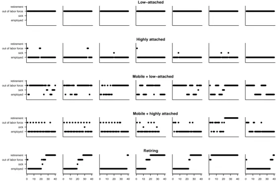
0 10 20 30 40 0 10 20 30 40 0 10 20 30 40
Figure 1: Employment profiles of typical cluster members within each cluster, showing the 10th, 25th, 50th, 70th, 100th, 200th and 350th highest classification probabilities.
4.2 Posterior Classification
As mentioned at the end of Section 3, we estimate the latent cluster indicatorsS= (S1, . . . , SN) jointly with the unknown cluster-specific parameters θH = (ϑ1, . . . ,ϑH,β2, . . . ,βH), by sam- pling from the posterior distribution p(θH,S|y). Parameter estimation is then based on the marginal posterior distribution p(θH|y) which is integrated over the unknown latent cluster in- dicatorsS. Within full conditional Gibbs sampling, soft clustering is performed implicitly (see classification rule (8) in Appendix A) and each worker impacts the estimates of all cluster-specific transition matrices, weighted according to his probability to belong to a certain cluster.
To obtain a first understanding of the transition patterns in the various clusters, the posterior draws are post-processed and hard clustering is performed for all individuals. Individuals are assigned to the five clusters of career-patterns using the posterior classification probabilities tih(θ5) = Pr(Si =h|yi,X =xi,θ5) given by eq. (8) in Appendix A. The posterior expectation ˆtih = E(tih(θ5)|y) of these probabilities is estimated by evaluating and averaging tih(θ5) over all MCMC draws of θ5. Each worker is then allocated to that cluster ˆSi, which exhibits the maximum posterior probability, i.e. ˆSi is defined such that ˆti,Sˆi = maxhˆtih. This decision rules minimizes the misclassification risk for each worker, see e.g. Fr¨uhwirth-Schnatter (2006, Section 7.1). The closer ˆti,Sˆ
i is to 1, the higher is the segmentation power for individual i.
Typical group members are visualized in Figure 1 for each cluster through their individual time series. The career patterns in Figure 1 are fairly similar within each cluster, but very different across clusters.
Low−attached: 21 %
Highly attached:
44 %
Mobile + low−attached: 8 % Mobile + highly attached: 7 %
Retiring: 20 %
Low−attached: 16 % Highly attached:
55 %
Mobile + low−attached: 4 % Mobile + highly attached: 4 %
Retiring: 21 %
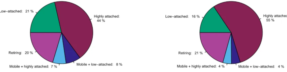
Figure 2: Group sizes for the five cluster solution. The cluster sizes are calculated based on the posterior classification probabilities. Left hand side: workers experiencing plant closure (displaced); right hand side: workers from the control group not experiencing plant closure
Based on the posterior classification probabilities of cluster membership for each of the N workers, we compute the average size of each cluster. The corresponding shares of individuals in each cluster are shown in the left hand graph of Figure 2. The displaced workers in our sample are relatively unevenly distributed across the five clusters: 21 % of the persons belong to clusterLow-attached, 44 % to clusterHighly attached, 8 % to clusterMobile + low- attached, 7 % to cluster Mobile + highly attached, and 20 % to cluster Retiring. 4.3 Analyzing Career Mobility
To analyze career mobility patterns in the five different clusters we investigate for each clus- ter the posterior distribution of the time-varying cluster-specific transition matrices ϑh = (πh,ξh1, . . . ,ξh,10) forh= 1, . . . ,5. For all workers in our sample, the transition process starts with the shock of job displacement due to plant closure. Thus the vector πh defines, for each cluster, the worker’s state distribution πh,1 = πh at the end of the first quarter after plant closure. The corresponding posterior expectation E(πh,1|y) is shown for each cluster in Figure 3 att= 1.
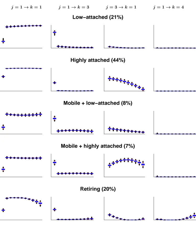
The time-varying cluster-specific transition matrices are visualized in Figure 4, with each of the five rows corresponding to a specific cluster. The four columns of Figure 4 correspond to transition probabilities of particular interest, namely persistence in the employment state (i.e. j = 1 → k = 1), transition from employment to out of labor force (i.e. j = 1 → k = 3), transition from out of labor force back to employment (i.e. j = 3 → k = 1), and transition from employment to retirement (i.e. j = 1→ k = 4). Each single plot in Figure 4 shows how the posterior distribution of the transition probability ξhy,jk from j → k changes in cluster h over time as the yearly distance from plant closure y = 1, . . . ,10 increases. Note that each posterior distributionp(ξhy,jk|y) is represented by box plots of the corresponding MCMC draws.
Furthermore, numerical estimates and standard deviations for the initial distributionπh as well as the above selected transition probabilitiesξhy,jk are reported in Table 3.
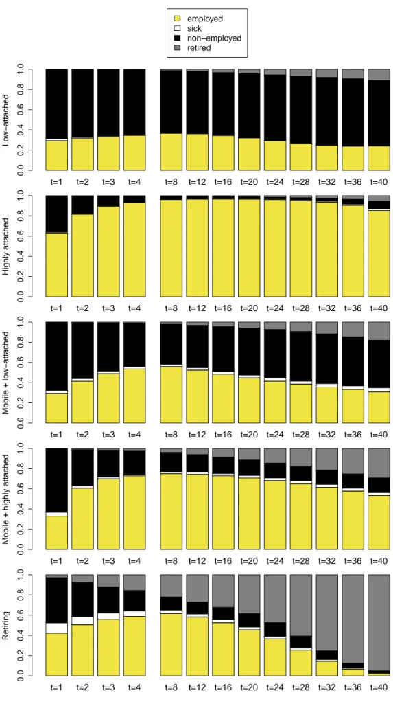
To evaluate the long-term effect of the job loss experienced by all workers, the state distri- bution πh,t was computed also for all subsequent quarters t = 2, . . . ,40, individually for each cluster. Given the distribution of states at the end of the first quarter, described by πh, each state distribution πh,t is computed by taking into account that the transition process evolves according to a time-inhomogenous Markov process:
πh,t =πhξh,1→t, h= 1, . . . , H. (5)
Starting fromξh,1→2:=ξh1, the transition matrixξh,1→tfrom the first to theqth quarter in year y, i.e. t= 4(y−1)+q, can be computed fort= 3, . . . ,40 recursively from the sequence of cluster- specific time-inhomogenous transition matrices throughξh,1→t=ξh,1→(t−1)ξhy. Figure 3 shows the evolution of the posterior expectations E(πh,t|y) of the cluster-specific state distribution over distance tfrom plant closure.3
4.4 Understanding the Clusters
In this subsection we present a synthesis of posterior inference in Figure 1 to Figure 4 and Table 3 and interpret the estimated transition processes after job displacement for the different clusters. The figures highlight remarkable differences across clusters in the state distribution at the end of the first quarter, as well as in the subsequent transition patterns. We will now discuss these career patterns cluster by cluster.
Cluster Highly attached is the largest one with about 44% of the observations. Workers in this cluster have a relatively high probability to be employed again within one quarter after plant closure (63%), whereas this probability is considerably smaller for all other clusters. Only 35.9% of the cluster members are still out of labor force one quarter after plant closure. For workers in this cluster, the probability to remain employed is close to 1 over the whole 10 years (98.9% five and 97.8% ten years after plant closure). As a consequence, for workers in this cluster the risk of another job loss is very small (0.7% five and 1.5% ten years after plant closure). In the unlikely event that these workers lose their job, they have quite a good chance to move back into employment within one quarter, however, with increasing distance from plant closure, this chance declines and is as small as 7.1% after 10 years.
Workers in cluster Low-attached, the second largest one containing about 21% of the sample, are less successful than workers in cluster Highly attached in finding a new job in the first quarter after plant closure (only about 30%) and the majority (68.4%) are still out of labor force. Similar numbers can be observed for workers in clusterMobile + low-attached and cluster Mobile + highly attached. Overall, workers in these three clusters suffer from the plant closure at least in the short run. However, what distinguishes workers in clusterLow- attached from workers in the other two clusters is the subsequent transition behavior. Most strikingly, among workers in clusterLow-attachedthe chance of moving from out of labor force back into employment is extremely low in the years following plant closure and even decreases,
3The posterior expectation is estimated by computingπh,t fort= 1, . . . ,40 for all 15 000 MCMC draws and averaging the resulting draws ofπh,t for each quartertand each clusterh.
being equal to only 1.3% five and 1% ten years after plant closure. Members of this cluster hardly ever move back into employment after having lost their job due to plant closure and suffer from plant closure also in the long run.
While the clustersMobile + low-attachedandMobile + highly attachedare similar to cluster Low-attached in the short-run after plant closure, they different from this cluster substantially in their subsequent transition pattern between out of labor force and employment.
Workers in these two clusters recover more easily from job displacement and have about the same probability of remaining employed, which is nearly constant over time and, on average, equal to 82%. They have a similar transition pattern from employment back to out of the labor force, which again is nearly constant over time and is, on average, equal to about 15%. Obviously, members in these two clusters have a good chance to move back into the labor market after plant closure, but they are at a high risk to lose their job again. Workers in these two clusters which are characterized by frequent switches between employment and being out of labor force suffer from an intrinsically high risk of being out of labor force that appears to be unrelated to plant closure.
The main distinction between cluster Mobile + highly attached and cluster Mobile + low-attachedis the transition pattern from out of labor force back into employment and how it evolves with distance from plant closure. This difference leads to career paths that are quite distinctive. For workers in cluster Mobile + highly attached, the chance of moving back into the labor market is higher than in the other cluster and even increases in the first five years after plant closure. The corresponding transition probability is as large as 74% five years and still equal to 54% ten years after plant closure. This leads to career patterns that are characterized by frequent transitions between employment and out of labor force, see also some typical members of this cluster in Figure 1. For cluster Mobile + low-attached, the transition probability from out of labor force back into employment is much smaller and declines, being only 15% five years and as small as 7.8% ten years after plant closure. Workers in both clusters switch between employment and being out of labor force; however, workers in cluster Mobile + low-attached have a much higher risk to remain out of labor force. As a consequence, this leads to much longer spells of being out of labor force than for workers in cluster Mobile + highly attached, where this duration is very short, see again Figure 1.
Finally, workers in cluster Retiring are less successful than workers in cluster Highly attachedto find a job in the first quarter after plant closure (42.2%), but more successful than workers in the other clusters. In cluster Retiring immediate transition into retirement after plant closure happens with positive probability (2.7%), whereas this probability is practically zero for all other clusters. Workers in this cluster also have a much higher risk (10.1%) to be on sick leave immediately after plant closure. In addition, we find an increasing transition probability from employment into retirement which is as large as 18.7% ten years after plant closure, whereas this probability practically remains zero for all other clusters. As a consequence, the probability to remain employed, which is relatively high in the first years after plant closure, declines in later years and is the smallest among all clusters (72.2%) after 10 years.
t=1 t=2 t=3 t=4 t=8 t=12 t=16 t=20 t=24 t=28 t=32 t=36 t=40 Low−attached 0.00.20.40.60.81.0
employed sick
non−employed retired
t=1 t=2 t=3 t=4 t=8 t=12 t=16 t=20 t=24 t=28 t=32 t=36 t=40 Highly attached 0.00.20.40.60.81.0
t=1 t=2 t=3 t=4 t=8 t=12 t=16 t=20 t=24 t=28 t=32 t=36 t=40 Mobile + low−attached 0.00.20.40.60.81.0
t=1 t=2 t=3 t=4 t=8 t=12 t=16 t=20 t=24 t=28 t=32 t=36 t=40 Mobile + highly attached 0.00.20.40.60.81.0
t=1 t=2 t=3 t=4 t=8 t=12 t=16 t=20 t=24 t=28 t=32 t=36 t=40 Retiring 0.00.20.40.60.81.0
Figure 3: Posterior expectation of the distributionπh,t over the 4 states (1 = employed, 2 = sick leave, 3 = out of labor force, 4 = retired) after a period of t quarters in the various clusters (workers experiencing plant closure).
j = 1→k = 1 j = 1→k = 3 j = 3→k = 1 j = 1→k = 4
Low−attached (21%)
Highly attached (44%)
Mobile + low−attached (8%)
Mobile + highly attached (7%)
Retiring (20%)
Figure 4: Visualization of the posterior distribution of four selected time-varying transition probabilities from state j to state k in the various clusters, with each row corresponding to a specific cluster. The first box plot in columns 1, 2 and 4 displays the posterior distribution of the state probability πh,k at the end of the first quarter after plant closure for each cluster h.
The remaining ten box plots display the posterior distribution of the transition probabilities ξhy,jk over the years y= 1,2, . . . ,10 for each cluster h. 1 = employed, 2 = sick leave, 3 = out of
The importance of using a time-inhomogeneous rather than a time-homogeneous Markov chain clustering method for our application can be best seen in Figure 3, which shows for each cluster how the state distribution evolves over time. The largest changes can be seen in the clusters Retiringand Mobile + low-attached, which is due to the varying importance of the states employment and retirement. The inhomogeneous modeling approach deals with such non-linear patterns in a very flexible way. Our time series data, where a stable equilibrium process is shocked by a plant closure, require flexibility in particular at the beginning. The importance of allowing for a separate transition process in the first quarter can clearly be seen in the large turbulence in the first year in Figure 3.
h πh,1 πh,2 πh,3 πh,4
Low-attached 0.292 (0.021) 0.021 (0.005) 0.684 (0.022) 0.002 (0.002) Highly attached 0.630 (0.011) 0.010 (0.002) 0.359 (0.011) 0.001 (0.001) Mobile + low-attached 0.294 (0.026) 0.030 (0.010) 0.672 (0.028) 0.003 (0.004) Mobile + highly attached 0.330 (0.026) 0.038 (0.012) 0.627 (0.027) 0.005 (0.006) Retiring 0.422 (0.016) 0.101 (0.009) 0.449 (0.016) 0.027 (0.005)
yeary j = 1→k= 1 j= 1→k= 3 j= 3→k= 1 j= 1→k= 4 Low-attached
y= 1 0.918 (0.009) 0.077 (0.009) 0.062 (0.005) 0.001 (0.001) y= 5 0.956 (0.006) 0.037 (0.005) 0.013 (0.002) 0.005 (0.001) y= 10 0.974 (0.006) 0.024 (0.005) 0.010 (0.002) 0.000 (0.000)
Highly attached
y= 1 0.978 (0.002) 0.019 (0.001) 0.545 (0.022) 0.000 (0.000) y= 5 0.989 (0.001) 0.007 (0.001) 0.416 (0.022) 0.000 (0.000) y= 10 0.978 (0.001) 0.015 (0.001) 0.071 (0.019) 0.000 (0.000)
Mobile + low-attached
y= 1 0.860 (0.014) 0.130 (0.013) 0.232 (0.020) 0.001 (0.001) y= 5 0.817 (0.012) 0.158 (0.010) 0.154 (0.013) 0.001 (0.001) y= 10 0.856 (0.018) 0.117 (0.016) 0.078 (0.009) 0.001 (0.001)
Mobile + highly attached
y= 1 0.841 (0.012) 0.146 (0.012) 0.506 (0.024) 0.003 (0.001) y= 5 0.821 (0.008) 0.158 (0.007) 0.740 (0.019) 0.003 (0.001) y= 10 0.822 (0.013) 0.146 (0.011) 0.540 (0.037) 0.005 (0.002)
Retiring
y= 1 0.938 (0.007) 0.021 (0.004) 0.221 (0.012) 0.021 (0.005) y= 5 0.955 (0.004) 0.024 (0.003) 0.011 (0.003) 0.000 (0.000) y= 10 0.722 (0.031) 0.052 (0.012) 0.040 (0.009) 0.187 (0.027) Table 3: Posterior expectations E(πh,k|y) and, in parenthesis, posterior standard deviations SD (πh,k|y) of the state probability πh,k at the end of the first quarter after plant closure for all statesk= 1, . . . ,4 as well as posterior expectations E(ξhy,jk|y) and, in parenthesis, posterior standard deviations SD (ξhy,jk|y) of selected transition probabilities ξhy,jk for selected years y in the various clusters. 1 = employed, 2 = sick leave, 3 = out of labor force, 4 = retired.
4.5 The Impact of Observables on Group Membership
After having established differences in labor market careers following plant closure across five different clusters of workers, we now investigate how individual characteristics relate to cluster membership. From a social policy point of view, it is interesting to understand if the character- istics of a particular worker make him more prone to belong to a specific cluster. In particular, we would like to answer questions such as: Is the career adjustment after plant closure easier for younger workers than for older workers? Who might be forced into early retirement? Do blue collar workers have a higher risk to belong to the most disadvantaged cluster Low-attached than white collar workers?
The mixture-of-experts approach allows to answer these and similar questions, since we specify the probability of an individual to belong to a certain cluster by the multinomial logit (MNL) model given in equation (4). The regression framework flexibly controls for the impact of six covariates in the MNL model, namely age at the time of plant closure, experience, broad occupational status (i.e. blue versus white collar), income, firm size, and the economic sector, each with dummy coding. More specifically, we introduce five age groups (35-39, 40-44, 45- 49, 50-55), three levels of experience (low, medium, high), a dummy for white-collar workers, three levels of income before plant closure (low, medium, high) based on the tertiles of the general income distribution at time of plant closure, three categories of firm size (1-10, 11-100, and more than 100 employees), and four broad economic sectors (service, industry, remaining seasonal business (outside of hotel and construction), unknown); see also Table 1. Alternatively, it would be possible to include all continuous covariates in the mixture-of-experts approach without discretization, as exemplified by a related paper on mothers’ long-run career patterns after first birth (Fr¨uhwirth-Schnatter et al., 2016) which uses a time-homogeneous mixture-of- experts Markov chain clustering approach.
Bayesian inference for the regression parameters βh in the MNL model (4) is summarized in Table 4, which reports the posterior expectation and the posterior standard deviation of all regression parameters relative to the baseline, which is equal to cluster Low-attached.
To visualize the main results, Figure 5 shows to which extent the probability of belonging to each of the five clusters is related to each individual covariate Xj; see also Table 5. For this evaluation, all covariates in X apart from Xj are set to their mean values observed in the sample. The probability Pr(Si = h|β2, . . . ,βH,X) that a worker with certain predetermined characteristicsXbelongs to clusterhis computed for all MCMC draws and the reported values are averages over all MCMC draws. Since the probabilities Pr(Si =h|β2, . . . ,βH,X) act as a
“prior” probabilities in the Bayes’ classification rule (8), as outlined in Appendix A, the various diagrams in Figure 5 can be interpreted as providing the prior probability that a worker belongs to any of the five clusters based solely on characteristics Xknown before plant closure.
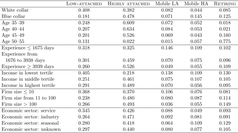
A worker’s broad occupational status is highly related to cluster membership; see Figure 5, panel (a), as well as Table 5. Most strikingly, blue collar workers have about half the risk of white collar workers (18% versus 41%) to belong to cluster Low-attached, which suffers most from plant closure. This is a specific feature of plant closure events, see also Schwerdt et al. (2010). Not surprisingly, white collar workers have a small prior probability to belong to cluster Mobile + highly attached(4%).
With respect to age at the time of plant closure, we see in Figure 5, panel (b), as well as in
Highly attached Mobile Mobile Retiring + low-attached + highly attached
Intercept -1.522 (0.177) -0.762 (0.249) -3.002 (0.261) -4.114 (0.294)
Age 35–39 (basis)
Age 40–44 0.220 (0.106) 0.334 (0.163) 0.201 (0.175) 0.307 (0.323)
Age 45–49 0.061 (0.118) 0.160 (0.186) 0.001 (0.196) 2.398 (0.246)
Age 50–55 -2.740 (0.388) -0.988 (0.436) 0.725 (0.236) 4.410 (0.249)
Experience ≤1675 days (basis) Experience from
1676 to 3938 days 0.404 (0.107) -0.687 (0.163) -0.318 (0.164) -0.010 (0.172) Experience ≥3939 days 0.687 (0.108) -0.891 (0.190) -0.490 (0.176) 0.272 (0.163)
Blue collar 1.045 (0.111) 0.665 (0.183) 2.020 (0.179) 1.212 (0.166)
Income in lowest tertile (basis)
Income in middle tertile 1.235 (0.156) -0.134 (0.197) 0.469 (0.191) 0.274 (0.202) Income in highest tertile 1.146 (0.153) -0.352 (0.186) -0.334 (0.213) 0.022 (0.201) Firm size ≤10 (basis)
Firm size from 11 to 100 0.701 (0.100) 0.163 (0.159) 0.578 (0.155) 0.787 (0.157) Firm size >100 0.617 (0.142) -0.761 (0.286) -0.002 (0.233) 0.941 (0.190) Economic sector: service (basis)
Economic sector: industry 0.368 (0.114) 0.314 (0.173) 0.785 (0.193) 0.253 (0.173) Economic sector: seasonal -0.224 (0.318) -0.065 (0.490) 0.588 (0.534) 0.282 (0.465) Economic sector: unknown 0.188 (0.103) -0.110 (0.164) 1.017 (0.179) 0.542 (0.165)
Table 4: Multinomial logit model to explain cluster membership in a particular cluster (base- line: Low-attached); the numbers are the posterior expectation and, in parenthesis, the posterior standard deviation of the various regression coefficients.
Table 5 that workers younger than 45 years have similar probabilities to belong to the various clusters. In particular, their probability to belong to clusterRetiringis low, but this probability strongly increases with age. Individuals with higher age more often belong to clusterRetiring, and this probability is particularly high (77%) for the oldest group, aged 50-55. At the same time, the probability of being in cluster Highly attached reduces with age and is negligible for the oldest age group. The probability to belong to cluster Mobile + highly attached is practically independent of age and the probability of belonging to cluster Low-attachedis slightly decreasing with age.
Work experience is less strongly related to cluster membership than age; see Figure 5, panel (c), and Table 5. We see that the five clusters are quite evenly distributed among individuals with low level of work experience. On the other hand, higher experience levels are correlated with a higher probability to belong to cluster Highly attached and a lower probability to belong to cluster Mobile + low-attached. Interestingly, the probability of belonging to cluster Retiringis practically independent of the amount of work experience.
The influence of pre-displacement income, measured in tertiles of the income distribution, can be studied in Figure 5, panel (d); see also Table 5. Low income workers have a particularly high probability to belong to cluster Low-attached and, at the same time, a comparably low probability to belong to cluster Highly attached. For the other income groups, cluster
membership resembles that of medium and high experience.
Figure 5, panel (e) and (f), as well as Table 5 show that cluster membership also varies with the size and industry affiliation of the firms from which workers are displaced. The groups with the largest portion in clusterLow-attachedare workers from small firms and from the service sector. The largest portion in clusterMobile + highly attachedis exhibited by the workers of medium size firms and workers from seasonal business outside of hotel and construction.
Low-attached Highly attached Mobile LA Mobile HA Retiring
White collar 0.408 0.382 0.082 0.044 0.085
Blue collar 0.181 0.478 0.071 0.145 0.125
Age 35–39 0.248 0.609 0.072 0.052 0.018
Age 40–44 0.207 0.634 0.084 0.053 0.021
Age 45–49 0.201 0.526 0.069 0.043 0.160
Age 50–55 0.131 0.022 0.015 0.057 0.775
Experience ≤1675 days 0.318 0.325 0.146 0.109 0.102
Experience from
1676 to 3938 days 0.301 0.459 0.070 0.075 0.096
Experience ≥3939 days 0.260 0.526 0.049 0.055 0.109
Income in lowest tertile 0.405 0.218 0.138 0.109 0.130
Income in middle tertile 0.251 0.461 0.075 0.107 0.105
Income in highest tertile 0.291 0.489 0.070 0.056 0.095
Firm size≤10 0.368 0.370 0.106 0.076 0.081
Firm size from 11 to 100 0.238 0.480 0.080 0.087 0.114
Firm size> 100 0.266 0.493 0.036 0.055 0.149
Economic sector: service 0.345 0.426 0.088 0.049 0.093
Economic sector: industry 0.264 0.471 0.092 0.081 0.091
Economic sector: seasonal 0.280 0.418 0.064 0.109 0.129
Economic sector: unknown 0.297 0.440 0.080 0.077 0.105
Table 5: Displaced workers: cluster membership probabilities for a single covariate. All other covariates are set to their mean values observed in the sample.
4.6 Comparison to the control group
After analyzing the career paths of displaced workers in the five different clusters, we now turn to a comparison of the careers of displaced workers with the control group of workers not affected by a plant closure. This gives us some insights in the counterfactual situation that would have arisen, if the plant closure had not taken place. The literature on job displacements typically compares mean post-displacement outcomes among displaced workers with those in a control group of non-displaced worker (Jacobson et al., 2005). Our objective is more complex, as we want to create a separate counterfactual scenario for each cluster group and compare the mean outcome in each group with the counterfactual. To achieve this goal, we propose a novel method that relies on posterior classification of control individuals based on the clustering model that we estimated for the displaced workers. In the following, we describe the corresponding classification of the controls and the simulation of the counterfactual career patterns in each cluster.
White collar Blue collar Prior probability to belong to a certain class 0.00.20.40.60.81.0
Low−attached Highly attached Mobile + low−attached Mobile + highly attached Retiring
35−39 40−44 45−49 50−55
Prior probability to belong to a certain class 0.00.20.40.60.81.0
Low−attached Highly attached Mobile + low−attached Mobile + highly attached Retiring
(a) (b)
Low Medium High
Prior probability to belong to a certain class 0.00.20.40.60.81.0
Low−attached Highly attached Mobile + low−attached Mobile + highly attached Retiring
Low Medium High
Prior probability to belong to a certain class 0.00.20.40.60.81.0
Low−attached Highly attached Mobile + low−attached Mobile + highly attached Retiring
(c) (d)
Low Medium High
Prior probability to belong to a certain class 0.00.20.40.60.81.0
Low−attached Highly attached Mobile + low−attached Mobile + highly attached Retiring
Service Industry Seasonal N/A
Prior probability to belong to a certain class 0.00.20.40.60.81.0
Low−attached Highly attached Mobile + low−attached Mobile + highly attached Retiring
(e) (f)
Figure 5: Impact of each covariate on the probability of a worker to belong to a certain cluster:
(a) occupational state, (b) age, (c) experience, (d) income at time of plant closure, (e) firm size, (f) firm’s economic sector (for each single covariate, all other covariates are set to their mean values observed in the sample). For each covariate, the probabilities of belonging to, respectively, cluster Low-attached, Highly attached, Mobile + low-attached, Mobile + highly attachedand Retiring are stacked from bottom to the top.