IHS Economics Series Working Paper 324
October 2016
Analysing Plant Closure Effects Using Time-Varying Mixture-of- Experts Markov Chain Clustering
Sylvia Frühwirth-Schnatter
Stefan Pittner
Andrea Weber
Rudolf Winter-Ebmer
Impressum Author(s):
Sylvia Frühwirth-Schnatter, Stefan Pittner, Andrea Weber, Rudolf Winter-Ebmer Title:
Analysing Plant Closure Effects Using Time-Varying Mixture-of-Experts Markov Chain Clustering
ISSN: 1605-7996
2016 Institut für Höhere Studien - Institute for Advanced Studies (IHS) Josefstädter Straße 39, A-1080 Wien
E-Mail: o ce@ihs.ac.at ffi Web: ww w .ihs.ac. a t
All IHS Working Papers are available online: http://irihs. ihs. ac.at/view/ihs_series/
This paper is available for download without charge at:
https://irihs.ihs.ac.at/id/eprint/4078/
Analysing Plant Closure Effects Using Time-Varying Mixture-of-Experts Markov Chain Clustering
Sylvia Fr¨uhwirth-Schnatter ∗ Stefan Pittner † Andrea Weber ‡ Rudolf Winter-Ebmer §
September 3, 2016
Abstract
In this paper, we study data on discrete labor market transitions from Austria. In particular, we follow the careers of workers who experience a job displacement due to plant closure and observe – over a period of forty quarters – whether these workers manage to return to a steady career path. To analyse these discrete-valued panel data, we develop and apply a new method of Bayesian Markov chain clustering analysis based on inhomogeneous first order Markov transition processes with time-varying transition matrices. In addition, a mixture-of-experts approach allows us to model the prior probability to belong to a certain cluster in dependence of a set of covariates via a multinomial logit model. Our cluster analysis identifies five career patterns after plant closure and reveals that some workers cope quite easily with a job loss whereas others suffer large losses over extended periods of time.
Keywords: Transition data, Markov Chain Monte Carlo, Multinomial Logit, Panel data, Inhomogeneous Markov chains
1 Introduction
Long-term career outcomes after job loss due to a plant closure – where all workers are auto- matically displaced – are an often researched topic in labor economics, see e.g. Jacobson et al.
(1993), Fallick (1996), Ruhm (1991) or more recently, for Austria, Ichino et al. (2016). Such a situation ideally allow us to observe how an economy absorbs exogenous shocks and how indi- viduals react to perturbations to their stable career path. A plant closure has the advantage that displaced workers are neither predominantly ones who are dismissed nor those changing jobs voluntarily: a plant closure is close to an exogenous event where everybody gets displaced.
In the present paper, we consider data on discrete labor market transitions from Austria.
In particular, we follow the careers of workers who experience a job displacement due to plant closure and observe – over a period of forty quarters – whether these workers manage to return to a steady career path. We can classify labor market states by quarter as being employed, sick, out of labor force, or retired.
∗ Institute for Statistics and Mathematics, Vienna University of Economics and Business
† Institute for Statistics and Mathematics, Vienna University of Economics and Business
‡ Department of Economics, Vienna University of Economics and Business and WIFO, Vienna
§ Department of Economics, Johannes Kepler University Linz and IHS, Vienna
Modelling transitions between discrete states over time is of interest not only in labor eco- nomics, but in many other areas of applied research such as demography, finance, mathematical biology or genetics. Examples of topics to which these models are applied span a wide range:
transitions between demographic states over the life cycles of individuals or households, tran- sitions between organisational characteristics, stock market participation or trading status of firms, changes in climate conditions across regions over time, or transitions of genetic determi- nants over generations of different species. These transition processes are typically captured by observations of unit-specific time series of discrete states over a longitudinal component.
When analyzing the effect of plant closure on career patterns in our specific application, we expect that unobserved heterogeneity in the response to job displacement from plant closure is present in the data. To account for unobserved heterogeneity and to identify subgroups of workers that follow similar transition patterns in our data set, which is a collection of several thousands of discrete-valued time series, we apply model-based clustering, see Banfield and Raftery (1993); Fraley and Raftery (2002); McNicholas and Murphy (2010); Gollini and Murphy (2014) among many others. For model-based clustering of discrete-valued time series, typically first order Markov chain models are used to model transitions between states and separate clusters are distinguished by different transition matrices, see Fr¨ uhwirth-Schnatter (2011) for a recent review.
Two important questions arise in this context. First, time-invariant or predetermined char- acteristics of a displaced worker may be correlated with group membership, i.e. persons with specific characteristics are more likely to belong to a certain cluster than to the other clus- ters. This issue can easily be addressed through the mixture-of-experts approach introduced by Peng et al. (1996), which allows to model the prior probability to belong to a specific cluster in dependence of covariates, see e.g. Gormley and Murphy (2008) for an application to model- based clustering of rank data, Fr¨ uhwirth-Schnatter and Kaufmann (2008) and Ju´ arez and Steel (2010) for an application to model-based clustering of time series of continuous outcomes and Fr¨ uhwirth-Schnatter et al. (2012) for an application to model-based clustering of discrete-valued time series. To obtain a better understanding which workers in our data set are inclined toward which career pattern, such a mixture-of-experts approach based on a multinomial logit model is applied to model the prior probability to belong to a certain cluster in dependence of control variables, such as the worker’s age at job displacement, the years of labor market experience, the occupational type (i.e. blue versus white collar), and the income in the quarter preceding the job displacement.
Second, previous approaches of Markov chain clustering of discrete-valued time series are typically based on time-homogeneous first order Markov chains, see e.g. Cadez et al. (2003);
Ramoni et al. (2002); Frydman (2005); Pamminger and Fr¨ uhwirth-Schnatter (2010). However, for our data the transition process is not necessarily stationary over time which poses an obvious challenge to time-invariant transition processes. An obvious reason for non-stationarity are the shocks to the stationary transition processes caused by an event out of the workers’ control, such as job displacement. In this case, the patterns of transition during the recovery phase may differ significantly from stationary transitions and we expect that after a plant closure the intrinsically stable transition process of workers in and out of jobs might be disturbed for a period of time.
Moreover, individual transitions will be shaped by changes over the life cycle – e.g. when it
comes to transitions towards sick leave or retirement as workers age over time.
To meet these challenges, we develop and apply a new method of Markov chain clustering and extend previous work on modelling transitions between labor market states through time- homogeneous Markov chain clustering. We extend the approach of Fr¨ uhwirth-Schnatter et al.
(2012) who introduced mixture-of-experts homogeneous Markov chain clustering for this type of time series by introducing inhomogeneous first order Markov transition processes with time- varying transition matrices as clustering kernels.
For our plant closure data, this new method of model-based cluster analysis identifies five career patterns after plant closure and reveals that some workers cope quite easily with a job loss whereas others suffer large losses over extended periods of time. By addressing this unobserved heterogeneity explicitly, our paper contributes to the labor economics literature by revealing a variety of different shock-absorption patterns across multiple clusters, while previous research concentrated only on average effects of job displacements
The paper proceeds as follows. The next section introduces the empirical problem and the data from Austrian social security registers. Section 3 introduces the time-varying Markov chain clustering model and discusses Bayesian statistical inference. Estimation results and im- plications for labor market careers after job displacement are discussed in Section 4. We first comment on model selection and posterior assignment of individual cluster memberships. Then we interpret the different clusters of labor market transition processes and discuss the relation- ship between cluster membership and observable individual characteristics. Finally, we compare labor market trajectories of displaced workers with those of a control group of individuals who do not experience a plant closure.
2 Data Description
Our empirical analysis is based on administrative register data from the Austrian Social Secu- rity Database (ASSD), which combines detailed longitudinal information on employment and earnings of all private sector workers in Austria (Zweim¨ uller et al., 2009). The data set includes the universe of private sector workers in Austria covered by the social security system. All employment spells record the identifier of the firm at which the worker is employed.
From the universe of employment records and employer identifiers, we can infer the char- acteristics of a firm’s workforce at any point in time. Importantly for our application, we can observe firm entries and exits. Specifically, we define a firm’s exit as the point in time when the last employee leaves a firm. This is a fully data-driven definition, which in some cases identifies employer exits that do not correspond to a plant closure, for example due to a firm takeover or due to an administrative reassignment of the employer identifier. In these cases, we observe that a large group of employees continue their employment with a new identifier. To get a more precise definition of plant closure, we therefore drop an observation from the set of firm exits, if more than 50% of the employees continue under a single new employer identification number. As this method relying on worker flows does not work well for firms with high seasonal employment fluctuations, we exclude the construction and tourism sectors from our analysis.
For the definition of our sample of displaced workers, we concentrate on all male workers
employed during the years 1982 to 1988, who were experiencing a job displacement due to plant
closure in this period. We follow these workers’ detailed labor market careers for 4 years prior
to job displacement and for 10 years afterwards. We further restrict the sample to workers displaced from firms that have more than 5 employees at least once during the period 1982 to 1988 and who have at least one year of tenure prior to displacement. Moreover, we select workers who were between 35 and 55 years of age at the time of job displacement, leading to the analysis windows being located before the official retirement age of 65 years in Austria. This procedure identifies 5,841 workers displaced by plant closures between 1982 and 1988.
To compare labor market careers after job loss with a counterfactual situation without job displacement, we extract a control group of workers who were employed during the years 1982 to 1988 in firms which do not close down. Our aim is to select controls who are very similar to the displaced group in terms of their pre-displacement labor market careers and observable individual characteristics. We therefore apply the following selection procedure. We start with the entire population of 1,087,705 male workers employed during the years 1982 to 1988 from which we draw a weighted sample of 5,841 workers, who are similar to the displaced group in terms of pre- displacement characteristics. Weights are constructed based on a logit regression estimating the probability of being displaced in the full set of displaced workers and potential controls (Imbens, 2004). The ASSD offers a rich set of covariates for this propensity score weighting procedure.
In particular, we control for employment and earnings information in the 4 years prior to job displacement as well as age, occupational type, firm size, and industry affiliation. Sampling weights based on the logit model assure that the distribution of pre-displacement characteristics is similar among displaced and control observations.
To model employment careers we proceed by constructing a quarterly time series of labor market states for each individual. Specifically, we define the following categories: 1 denotes employed, 2 sick leave, 3 out of labor force (registered as unemployed or otherwise out of labor force), 4 retired (claiming government pension benefits). Retirement is coded as an absorbing state as virtually nobody in Austria returns to employment once he/she enters the public pension system. These time series of labor market states are the basis of our empirical Markov chain clustering method.
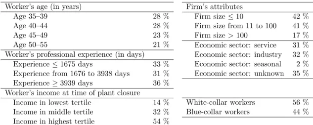
To study characteristics that are correlated with different career patterns after job loss, we focus on variables which are pre-determined at the time of plant closure. Control variables include the worker’s age at job displacement, the years of labor market experience, the occu- pational type (i.e. blue versus white collar), and the income in the quarter preceding the job displacement. Moreover, we control for firm size and industry. For computational reasons we transform all these variables into discrete categories; for summary statistics see Table 1.
3 Time-varying Mixture-of-Experts Markov Chain Clustering
As for many data sets available for empirical labor market research, the structure of the indi- vidual level transition data introduced in Section 2 takes the form of a discrete-valued panel data. The categorical outcome variable y it assumes one out of four states, labeled by { 1, 2, 3, 4 } , and is observed for N individuals i = 1, . . . , N over T i quarters for a maximum of 10 years, i.e.
T i ≤ 40 quarters. Moreover, we restrict ourselves to T i ≥ 4. For each individual i, we model
the state of the outcome variable y it in period t to depend on the past state y i,t−1 through a
time-inhomogeneous first order Markov transition model.
Worker’s age (in years)
Age 35–39 28 %
Age 40–44 28 %
Age 45–49 23 %
Age 50–55 21 %
Worker’s professional experience (in days)
Experience ≤ 1675 days 33 %
Experience from 1676 to 3938 days 31 %
Experience ≥ 3939 days 36 %
Worker’s income at time of plant closure
Income in lowest tertile 14 %
Income in middle tertile 32 %
Income in highest tertile 54 %
Firm’s attributes
Firm size ≤ 10 42 %
Firm size from 11 to 100 41 % Firm size > 100 17 % Economic sector: service 31 % Economic sector: industry 32 % Economic sector: seasonal 2 % Economic sector: unknown 35 %
White-collar workers 56 % Blue-collar workers 44 %
Table 1: Descriptive statistics for the control variables of all displaces persons in the mixture- of-experts model to explain group membership.
To capture the presence of unobserved heterogeneity in the dynamics in our discrete-valued panel data, we apply model-based clustering based on Markov transition models. The central assumption in model-based clustering is that the N time series in the panel arise from H hidden classes; see Fr¨ uhwirth-Schnatter (2011). Within each class, say h, all time series can be char- acterized by the same data generating mechanism, called a clustering kernel, which is defined in terms of a probability distribution for the time series y i = { y i1 , . . . , y i,T i } , depending on an unknown class-specific parameter ϑ h . A latent cluster indicator S i taking a value in the set { 1, . . . , H } is introduced for each time series y i to indicate which class the individual i belongs to, i.e. p(y i | S i , ϑ 1 , . . . , ϑ H ) = p(y i |ϑ S i ).
To address serial dependence among the observations for each individual i, model-based clustering of time series data is typically based on dynamic clustering kernels derived from first order Markov processes, where the clustering kernel p(y i |ϑ h ) = T i
t=1 p(y it | y i,t−1 , ϑ h ) is formu- lated conditional on the initial state y i0 , which in our application is equal to 1 (employed) for all individuals. For discrete-valued time series, persistence is typically captured by assuming that y i follows a time-homogeneous Markov chain of order one. Applications of time-homogeneous Markov Chain clustering to analyze individual wage careers in the Austrian labor market include Pamminger and Fr¨ uhwirth-Schnatter (2010), Pamminger and T¨ uchler (2011), and Fr¨ uhwirth- Schnatter et al. (2012).
However, the assumption that the long-run career paths of workers who experienced plant closure follow a time-homogeneous Markov chain is not realistic (see Ichino et al. (2016), Fig- ure 2). A descriptive investigation of the evolution of the employment rate over distance to plant closure reveals that the employment rate does not converge to a steady state, but rather declines steadily with increasing distance to plant closure. Homogeneity would imply that the employment rate as well as all other state probabilities converge to a steady state within the observation period, both within each cluster as well marginalized over all clusters.
To obtain such a non-stationary pattern, we need to assume that the transition probabilities
between the various states change with distance to plant closure. Furthermore, it is to be
expected that there is a lot of heterogeneity in this time-varying pattern across workers.
To capture this non-stationary feature of our data, we develop in the present paper Markov chain clustering based on a time-inhomogeneous first order Markov chain model with class- specific time-varying transition matrices ϑ h = ( π h , ξ h1 , . . . , ξ h10 ) as clustering kernel. More specifically, we assume that the transition behavior changes with distance to plant closure. Since the initial state is employment (i.e. y i0 = 1) for all workers, the first transition is described by the row vector π h = (π h,1 , . . . , π h,4 ), containing the cluster-specific probability distribution of the states y i1 at the end of the first quarter after plant closure. The transition matrix ξ h1 describes the transition behavior between the various states in quarter two to four after plant closure, while the remaining transition matrices ξ hy , y = 2, . . . , 10, describe the transition behavior for all four quarters in year y after plant closure. Since the fourth state, namely retirement, is an absorbing state, each of these time-varying transition matrices ξ hy consists of three rows ξ hy,j· = (ξ hy,j1 , . . . , ξ hy,j4 ), j = 1, 2, 3, representing a probability distribution over the states { 1, 2, 3, 4 } , i.e. 4
k=1 ξ hy,jk = 1. Hence the clustering kernel reads:
p(y i |ϑ h ) = p(y i,−1 | y i1 , ξ h1 , . . . , ξ h10 )p(y i1 | S i = h, π h ), (1) where the truncated time series y i,−1 = { y i2 , . . . , y i,T i } is described by time-varying transition matrices changing every year:
p(y i,−1 | y i1 , ξ h1 , . . . , ξ h10 ) = 10 y=1
3 j=1
ξ hy,jk N iy,jk , (2)
with transition probabilities ξ h1,jk = Pr(y it = k | y i,t−1 = j, S i = h, t ∈ { 2, 3, 4 } ), and ξ hy,jk = Pr(y it = k | y i,t−1 = j, S i = h, t ∈ { 4(y − 1) + 1, . . . , 4y } ) for y = 2, . . . , 10. For each time series y i,−1 , the cluster-specific sampling distribution (2) depends on the number of transitions from state j to state k observed in each year, i.e. N i1,jk = # { y i,t−1 = j, y it = k | t ∈ { 2, 3, 4 }} and N iy,jk = # { y i,t−1 = j, y it = k | t ∈ { 4(y − 1) + 1, . . . , 4y }} for y = 2, . . . , 10. If T i < 40, then all transition counts are zero for all unobserved quarters.
The choice of the distribution for the state y i1 at the end of the first quarter in (1) has to address the problem with initial conditions in non-linear dynamic models with unobserved heterogeneity, see e.g. Heckman (1981) and Wooldridge (2005). This issue is relevant for cases, where unobserved heterogeneity is either captured through an individual effect S i following a continuous distribution, but, as discussed in Fr¨ uhwirth-Schnatter et al. (2012), also for models where S i follows a discrete distribution as for model-based clustering based on transition models.
The key issue is to allow for dependence between the initial state y i1 and the latent variable S i , which can be achieved by allowing the prior distribution of S i to depend on y i1 , an approach that has been pursued for the analysis of labor market entry and earnings dynamics in Fr¨ uhwirth- Schnatter et al. (2012).
In the present paper, we factorize the joint distribution of y i1 and S i in a different way as
p(y i1 , S i |· ) = p(y i1 | S i , π S i )p(S i |β 2 , . . . , β H , x i ), where the entire initial state distribution changes
across the clusters, i.e.:
p(y i1 | S i = h, π h ) = 4 k=1
π h,k I i,k , (3)
where π h,k = Pr(y i1 = k | S i = h) and I i,k = I { y i1 = k } is an indicator for a worker’s state at the end of the first quarter after plant closure.
Following the mixture-of-experts approach introduced for Markov chain clustering methods by Fr¨ uhwirth-Schnatter et al. (2012), the prior distribution of the latent indicator S i is influenced by exogenous covariates and is modeled as following a multinomial logit (MNL) model:
Pr(S i = h |β 2 , . . . , β H , x i ) = exp (x i β h ) 1 + H
l=2 exp (x i β l ) , h = 1, . . . , H, (4) where the row vector x i = (1, x i1 , . . . , x ir ) includes the constant 1 for the intercept in addition to the exogenous covariates (x i1 , . . . , x ir ). For identifiability reasons β 1 = 0, which means that h = 1 is the baseline class and β h is the effect on the log-odds ratio relative to the baseline.
For estimation, we pursue a Bayesian approach. For a fixed number H of clusters, Markov chain Monte Carlo (MCMC) methods are used, to estimate the latent cluster indicators S = (S 1 , . . . , S N ) along with the unknown cluster-specific parameters θ H = ( ϑ 1 , . . . , ϑ H , β 2 , . . . , β H ) from the data y = (y 1 , . . . , y N ). To sample from the posterior distribution p( θ H , S | y), we extend the sampler introduced in Fr¨ uhwirth-Schnatter et al. (2012) to time-inhomogeneous mixture-of- experts Markov chain clustering; see Appendix A for computational details.
4 Analysing Plant Closure Effects
To identify clusters of individuals with similar career patterns after plant closure, we apply Markov chain clustering for 2 up to 6 clusters. All computations are based on the prior distri- butions introduced in Appendix A. For each number H of clusters we simulate 15 000 MCMC draws after a burn-in of 10 000 draws and use them for all posterior inference reported below. 1
In the following, we start with a description of model selection and posterior classification.
Second, we discuss the cluster-specific post-displacement career patterns that are implied by the estimated transition processes. Third, we describe the correlation between cluster membership and workers’ characteristics. Finally, we compare the career paths of displaced workers with a control group who did not experience a job loss.
4.1 Model Selection
Statistical model selection criteria such as the AIC, the BIC or the AWE criterion as discussed e.g. in Fr¨ uhwirth-Schnatter (2011) could be applied to the present data to select the number H of clusters, however, these statistical criteria typically are not unambiguous and do not give a clear answer. For this reason, we select the number of clusters based on the economic interpretability
1 The computing time for all 25 000 draws is approx. 15 minutes for H = 2, 1 hour and 2 minutes for H = 3, 1
hour and 33 minutes for H = 4, 2 hours and 21 minutes for H = 5 and 4 hours and 45 minutes for H = 6 on a
Lenovo Thinkpad T410s laptop equipped with 4 GB RAM and an Intel Core i5 processor with 2.67 GHz.
of the different results. We choose the model where the clusters are sufficiently distinct, both in statistical terms as well as in terms of allowing a meaningful economic interpretation. As we will discuss below, we can conveniently interpret five distinct clusters of career patterns, which are characterized by a combination of mobility/persistence and attachment to the labor force: a Low-attached as well as a Highly attached cluster are characterized by low and high levels of attachment to the labor market, respectively, with high persistence in the corresponding states;
a Mobile + low-attached and a Mobile + highly attached cluster are characterized by a much higher level of mobility together with low and high levels of attachment to the labor market, respectively; and, finally, a cluster of Retiring , where retirement is the predominant state.
/RZíDWWDFKHG
+LJKO\DWWDFKHG
0RELOHORZíDWWDFK
HG
0RELOHKLJKO\DWWD
FKHG
0RVWW\SLFDOJURXS PHPEHUQXPEHU
0RVWW\SLFDOJURXS PHPEHUQXPEHU
0RVWW\SLFDOJURXS PHPEHUQXPEHU
5HWLULQJ
0RVWW\SLFDOJURXS PHPEHUQXPEHU
0RVWW\SLFDOJURXS PHPEHUQXPEHU
0RVWW\SLFDOJURXS PHPEHUQXPEHU
0RVWW\SLFDOJURXS PHPEHUQXPEHU
Figure 1: Employment profiles of typical cluster members within each cluster, showing the 10th, 25th, 50th, 70th, 100th, 200th and 350th highest classification probabilities. 1 = employed, 2 = sick, 3 = out of labor force, 4 = retirement.
In a six-cluster model, the distinctions between different clusters are less clear. Therefore, in the following, we concentrate on the five-cluster solution chiefly because this solution led to meaningful interpretations from an economic point of view.
4.2 Posterior Classification
Individuals are assigned to the five clusters of career-patterns using the posterior classification
probabilities t ih ( θ 5 ) = Pr(S i = h | y i , θ 5 ) given by eq. (8) in the Appendix. The posterior
expectation ˆ t ih = E(t ih ( θ 5 ) | y) of these probabilities is estimated by evaluating and averaging
t ih ( θ 5 ) over all MCMC draws of θ 5 . Each worker is then allocated to that cluster S ˆ i , which
exhibits the maximum posterior probability, i.e. ˆ S i is defined in such a way that ˆ t i, S ˆ
i = max h ˆ t ih . The closer ˆ t i, S ˆ
i is to 1, the higher is the segmentation power for individual i.
/RZíDWWDFKHG
+LJKO\DWWDFKHG
0RELOHORZíDWWDFKHG 0RELOHKLJKO\DWWDFKHG
5HWLULQJ
/RZíDWWDFKHG +LJKO\DWWDFKHG
0RELOHORZíDWWDFKHG 0RELOHKLJKO\DWWDFKHG
5HWLULQJ
Figure 2: Group sizes for the five cluster solution. The cluster sizes are calculated based on the posterior classification probabilities. Left hand side: workers experiencing plant closure (displaced); right hand side: workers not experiencing plant closure (controls)
To obtain a first understanding of the transition patterns in the various clusters, typical group members are selected for each cluster and their individual time series are plotted in Figure 1.
The career patterns are fairly similar within each cluster, but very different across clusters.
Based on the posterior classification probabilities of cluster membership for each of the N workers, we compute the average size of each cluster. The corresponding shares of individuals in each cluster are shown in the left hand graph of Figure 2. The displaced workers in our sample are relatively unevenly distributed across the five clusters: 21 % of the persons belong to the Low-attached , 44 % to the Highly attached , 8 % to the Mobile + low-attached , 7 % to the Mobile + highly attached , and 20 % to the Retiring cluster.
4.3 Analyzing Career Mobility
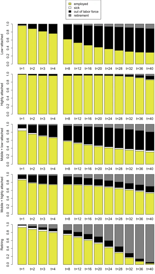
To analyze career mobility patterns in the five different clusters we investigate for each clus- ter the posterior distribution of the time-varying cluster-specific transition matrices ϑ h = ( π h , ξ h1 , . . . , ξ h10 ) for h = 1, . . . , 5. For all workers in our sample, the transition process starts with the shock of loosing employment due to plant closure. Thus the vector π h defines, for each cluster, the worker’s state distribution π h,1 = π h at the end of the first quarter after plant closure. The corresponding posterior expectation E( π h,1 | y) is shown for each cluster in Figure 3 at t = 1.
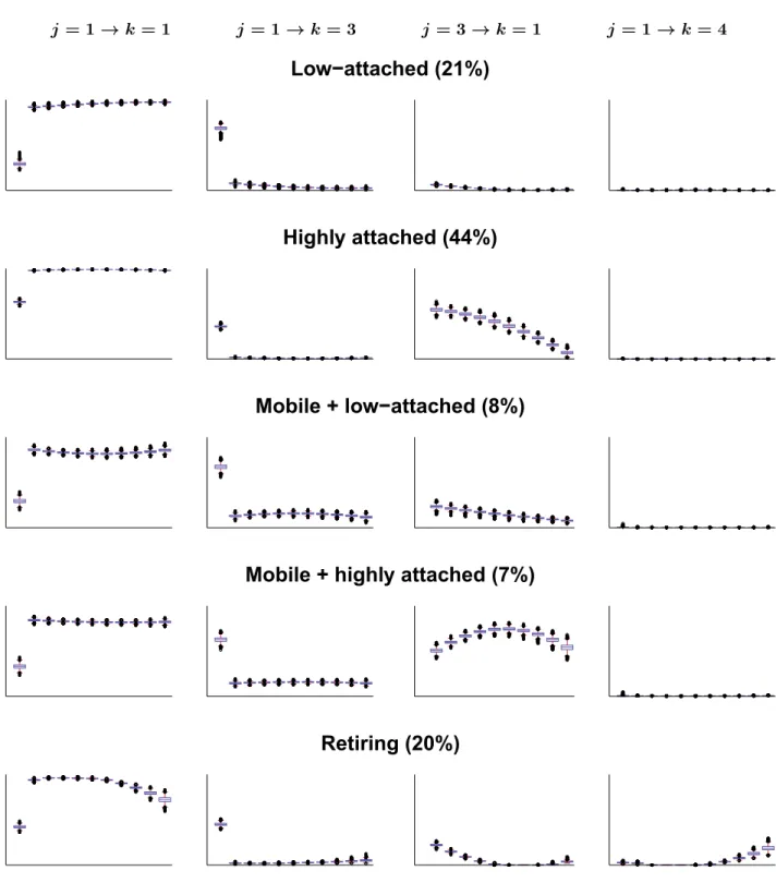
The time-varying cluster-specific transition matrices are visualized in Figure 4 for selected
transition probabilities of particular interest. In particular, the columns of Figure 4 display the
probabilities of following events: persistence in the employment state (i.e. j = 1 → k = 1),
transition from employment to out of labor force (i.e. j = 1 → k = 3), transition from out
of labor force back to employment (i.e. j = 3 → k = 1), and transition from employment to
retirement (i.e. j = 1 → k = 4). For each of the corresponding transition probabilities ξ hy,jk ,
the marginal posterior distribution p(ξ hy,jk | y) is represented for each of the five clusters by a
sequence of ten box plots of the corresponding MCMC draws, over the yearly distance to plant closure y = 1, . . . , 10.
The numerical estimates and standard deviations for the initial distribution π h as well as the above selected transition probabilities ξ hy,jk are reported in Table 2.
h π h,1 π h,2 π h,3 π h,4
Low-attached 0.292 (0.021) 0.021 (0.005) 0.684 (0.022) 0.002 (0.002) Highly attached 0.630 (0.011) 0.010 (0.002) 0.359 (0.011) 0.001 (0.001) Mobile + low-attached 0.294 (0.026) 0.030 (0.010) 0.672 (0.028) 0.003 (0.004) Mobile + highly attached 0.330 (0.026) 0.038 (0.012) 0.627 (0.027) 0.005 (0.006) Retiring 0.422 (0.016) 0.101 (0.009) 0.449 (0.016) 0.027 (0.005)
year y j = 1 → k = 1 j = 1 → k = 3 j = 3 → k = 1 j = 1 → k = 4 Low-attached
y = 1 0.918 (0.009) 0.077 (0.009) 0.062 (0.005) 0.001 (0.001) y = 5 0.956 (0.006) 0.037 (0.005) 0.013 (0.002) 0.005 (0.001) y = 10 0.974 (0.006) 0.024 (0.005) 0.010 (0.002) 0.000 (0.000)
Highly attached
y = 1 0.978 (0.002) 0.019 (0.001) 0.545 (0.022) 0.000 (0.000) y = 5 0.989 (0.001) 0.007 (0.001) 0.416 (0.022) 0.000 (0.000) y = 10 0.978 (0.001) 0.015 (0.001) 0.071 (0.019) 0.000 (0.000)
Mobile + low-attached
y = 1 0.860 (0.014) 0.130 (0.013) 0.232 (0.020) 0.001 (0.001) y = 5 0.817 (0.012) 0.158 (0.010) 0.154 (0.013) 0.001 (0.001) y = 10 0.856 (0.018) 0.117 (0.016) 0.078 (0.009) 0.001 (0.001)
Mobile + highly attached
y = 1 0.841 (0.012) 0.146 (0.012) 0.506 (0.024) 0.003 (0.001) y = 5 0.821 (0.008) 0.158 (0.007) 0.740 (0.019) 0.003 (0.001) y = 10 0.822 (0.013) 0.146 (0.011) 0.540 (0.037) 0.005 (0.002)
Retiring
y = 1 0.938 (0.007) 0.021 (0.004) 0.221 (0.012) 0.021 (0.005) y = 5 0.955 (0.004) 0.024 (0.003) 0.011 (0.003) 0.000 (0.000) y = 10 0.722 (0.031) 0.052 (0.012) 0.040 (0.009) 0.187 (0.027) Table 2: Posterior expectations E(π h,k | y) and, in parenthesis, posterior standard deviations SD (π h,k | y) of the state probability π h,k at the end of the first quarter after plant closure for all states k = 1, . . . , 4 as well as posterior expectations E(ξ hy,jk | y) and, in parenthesis, posterior standard deviations SD (ξ hy,jk | y) of selected transition probabilities ξ hy,jk for selected years y in the various clusters. 1 = employed, 2 = sick, 3 = out of labor force, 4 = retirement.
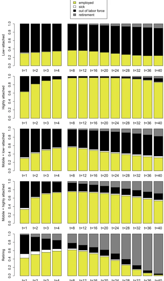
To evaluate the long-term effect of the job loss experienced by all workers, the state distri- bution π h,t was computed also for all subsequent quarters t = 2, . . . , 40, individually for each cluster. Given the distribution of states at the end of the first quarter, described by π h , each state distribution π h,t is computed by taking into account that the transition process evolves according to a time-inhomogenous Markov process:
π h,t = π h ξ h,1→t , h = 1, . . . , H. (5)
Starting from ξ h,1→2 := ξ h1 , the transition matrix ξ h,1→t from the first to the qth quarter in year
y, i.e. t = 4(y − 1)+q, can be computed for t = 3, . . . , 40 recursively from the sequence of cluster- specific time-inhomogenous transition matrices by ξ h,1→t = ξ h,1→(t−1) ξ hy . Figure 3 shows the evolution of the posterior expectations E( π h,t | y) of the cluster-specific state distribution over distance t to plant closure. 2
4.4 Understanding the Clusters
In this subsection we present a synthesis of posterior inference in Figure 1 to Figure 4 and Table 2 and interpret the estimated transition processes after job displacement for the different clusters. The figures highlight remarkable differences across clusters in the state distribution at the end of the first quarter, as well as in the subsequent transition patterns. We will now discuss these career patterns cluster by cluster.
Highly attached is the largest cluster with about 44% of the observations. Workers in this cluster have a relatively high probability to be employed again within one quarter after plant closure (63%), whereas this probability is considerably smaller for all other clusters. Only 35.9% of the cluster members are out of labor force one quarter after plant closure. For workers in this cluster, the probability to remain employed is close to 1 over the whole 10 years (98.9%
five and 97.8% ten years after plant closure). As a consequence, for workers in this cluster the risk of another job loss is very small (0.7% five and 1.5% ten years after plant closure). In the unlikely event that these workers loose their job, they have quite a good chance to move back into employment within one quarter, however, with increasing distance to plant closure, the chance declines and is as small as 7.1% after 10 years.
Workers in the Low-attached cluster, the second largest cluster covering about 21% of the sample, are less successful than Highly attached in finding a new job in the first quarter after plant closure (only about 30%) and the majority (68.4%) are still out of labor force. The pattern in the first quarter after plant closure is similar for workers in the Mobile + low-attached and Mobile + highly attached clusters. Workers in these three clusters obviously suffer from the plant closure, at least in the short run.
What distinguishes workers in Low-attached from Mobile + low-attached and Mo- bile + highly attached is the subsequent transition behavior. Most strikingly, among Low- attached workers the chance of moving from out of labor force back into employment is ex- tremely low in the years following plant closure and even decreases, being equal to only 1.3%
five and 1% ten years after plant closure. In contrast, workers in Mobile + low-attached and Mobile + highly attached recover more easily from job displacement. Members of Low-attached hardly ever move back into employment after having lost their job due to plant closure. However, in the unlikely event, that workers in this cluster find a job, they have quite a good chance to keep their job, and this chance is larger than for Mobile + low-attached and Mobile + highly attached .
While Mobile + low-attached and Mobile + highly attached are similar to Low- attached immediately after plant closure, they show a subsequent transition pattern between out of labor force and employment that is quite different. Both clusters have about the same probability of remaining employed, which is nearly constant over time and, on average, equal
2 The posterior expectation is estimated by computing π h,t for t = 1 , . . . , 40 for all 15 000 MCMC draws and
averaging the resulting draws of π h,t over all draws for each quarter t .
to 82%. They have a similar transition pattern from employment back into out of labor force, which again is nearly constant over time and is, on average, equal to about 15%. Members in both clusters have a good chance to move back into the labor market after plant closure, but they are at a high risk to loose their job again. These two clusters suffer from an intrinsically high risk of being out of labor force that appears to be unrelated to plant closure.
The main distinction between Mobile + low-attached and Mobile + highly attached is how the transition probability from out of labor force back into employment evolves with distance to plant closure. For workers in Mobile + highly attached the chance of moving back into the labour market is higher than in Mobile + low-attached and even increases in the first five years after plant closure. The corresponding transition probability is as large as 74% five years and still equal to 54% ten years after plant closure. This leads to career patterns that are characterized by frequent transitions between employment and out of labor force, see also the typical members in Figure 1.
While Mobile + low-attached is similar to Mobile + highly attached in several respects, it is mainly the transition pattern from out of labor force back into employment that leads to career paths that are quite distinctive from Mobile + highly attached . Evidently, for Mobile + low-attached the transition probability from out of labor force back into employment is much smaller than in Mobile + highly attached and even declines over distance to plant closure. The corresponding transition probability is only 15% five years and as small as 7.8% ten years after plant closure. Workers in this cluster also switch between employment and being out of labor force; however, they have a much higher risk to remain out of labor force than workers in Mobile + highly attached . As a consequence, this leads to much longer spells of being out of labor force than for workers in Mobile + highly attached , where this duration is very short, see again Figure 1.
Workers in the Retiring cluster are more successful than Low-attached , Mobile + low- attached , and Mobile + highly attached to find a job in the first quarter after plant closure (42.2%), but less successful than Highly attached . This is the only cluster where immediate transition into retirement after plant closure happens with positive probability (2.7%), whereas this probability is practically 0 for all other clusters. Workers in this cluster also have a much higher risk (10.1%) to be on sick leave immediately after plant closure than workers in all other clusters. In addition, this cluster is characterized by an increasing transition probability from employment into retirement which is as large as 18.7% ten years after plant closure. For all other clusters, this probability practically remains zero. As a consequence, the probability to remain employed, which is relatively high in the first five or six years after plant closure, declines in later years and is the smallest among all clusters (72.2%) after 10 years.
The importance of using a time-inhomogeneous rather than a time-homogeneous Markov
process for our application can be best seen in Figure 3 where the transition matrices change
over time in all clusters. The largest changes can be seen in the clusters Retiring and Mo-
bile + low-attached , which is due to the varying importance of the states employment and
retirement. The inhomogeneous modeling approach deals with such non-linear patterns in a
very flexible way. Our time series data, where a stable equilibrium process is shocked by a
plant closure, require flexibility in particular at the beginning. The importance of allowing for
a separate transition process in the first quarter can clearly be seen in the large turbulence in
the first year in Figure 3.
W W W W W W W W W W W W W
/R ZíDWWDFKHG
HPSOR\HG VLFN
RXWRIODERUIRUFH UHWLUHPHQW
W W W W W W W W W W W W W +LJKO\DWWDFKHG
W W W W W W W W W W W W W 0RELOHOR Z íDWWDFKHG
W W W W W W W W W W W W W 0RELOHKLJKO\DWWDFKHG
W W W W W W W W W W W W W
5HWLU LQJ
Figure 3: Posterior expectation of the distribution π h,t over the 4 states (1 = employed, 2 = sick,
3 = out of labor force, 4 = retirement) after a period of t quarters in the various clusters (workers
experiencing plant closure).
j = 1 → k = 1 j = 1 → k = 3 j = 3 → k = 1 j = 1 → k = 4
/RZíDWWDFKHG
+LJKO\DWWDFKHG
0RELOHORZíDWWDFKHG
0RELOHKLJKO\DWWDFKHG
5HWLULQJ
Figure 4: Visualization of the posterior distribution of 4 selected time-varying transition prob-
abilities from state j to state k in the various clusters, obtained by time-inhomogeneous Markov
chain clustering. The first box plot in columns 1, 2 and 4 displays the posterior distribution
of the state probability π h,k at the end of the first quarter after plant closure for each cluster
h. The remaining 10 box plots display the posterior distribution of the transition probabilities
ξ over the years y = 1, 2, . . . , 10 for each cluster h. 1 = employed, 2 = sick, 3 = out of labor
Highly attached Mobile Mobile Retiring + low-attached + highly attached
Intercept -1.522 (0.177) -0.762 (0.249) -3.002 (0.261) -4.114 (0.294)
Age 35–39 (basis)
Age 40–44 0.220 (0.106) 0.334 (0.163) 0.201 (0.175) 0.307 (0.323)
Age 45–49 0.061 (0.118) 0.160 (0.186) 0.001 (0.196) 2.398 (0.246)
Age 50–55 -2.740 (0.388) -0.988 (0.436) 0.725 (0.236) 4.410 (0.249)
Experience ≤ 1675 days (basis) Experience from
1676 to 3938 days 0.404 (0.107) -0.687 (0.163) -0.318 (0.164) -0.010 (0.172) Experience ≥ 3939 days 0.687 (0.108) -0.891 (0.190) -0.490 (0.176) 0.272 (0.163)
Blue collar 1.045 (0.111) 0.665 (0.183) 2.020 (0.179) 1.212 (0.166)
Income in lowest tertile (basis)
Income in middle tertile 1.235 (0.156) -0.134 (0.197) 0.469 (0.191) 0.274 (0.202) Income in highest tertile 1.146 (0.153) -0.352 (0.186) -0.334 (0.213) 0.022 (0.201) Firm size ≤ 10 (basis)
Firm size from 11 to 100 0.701 (0.100) 0.163 (0.159) 0.578 (0.155) 0.787 (0.157) Firm size > 100 0.617 (0.142) -0.761 (0.286) -0.002 (0.233) 0.941 (0.190) Economic sector: service (basis)
Economic sector: industry 0.368 (0.114) 0.314 (0.173) 0.785 (0.193) 0.253 (0.173) Economic sector: seasonal -0.224 (0.318) -0.065 (0.490) 0.588 (0.534) 0.282 (0.465) Economic sector: unknown 0.188 (0.103) -0.110 (0.164) 1.017 (0.179) 0.542 (0.165)
Table 3: Multinomial logit model to explain cluster membership in a particular cluster (base- line: Low-attached ); the numbers are the posterior expectation and, in parenthesis, the posterior standard deviation of the various regression coefficients.
4.5 The Impact of Observables on Group Membership
After having established differences in labor market careers following plant closure across five different clusters of workers, we are setting out to investigate how individual characteristics relate to cluster membership. From a social policy point of view, it is interesting to understand if the characteristics of a particular worker make him more prone to belong to a specific cluster.
In particular, we would like to answer questions such as: Is the career adjustment after plant closure easier for younger workers than for older workers? Who might be forced into early retirement? Do blue collar workers have a higher risk to belong to the Low-attached cluster than white collar workers?
The mixture-of-experts approach allows to answer these and similar questions, since we
specify the prior probability of an individual to belong to a certain cluster by the multinomial
logit (MNL) model given in equation (4). The regression framework controls for the impact of
six covariates in the MNL model, namely age at the time of plant closure, experience, broad
occupational status (i.e. blue versus white collar), income, firm size, and the economic sector,
each with dummy coding. More specifically, we introduce five age groups (35-39, 40-44, 45-
49, 50-55), three levels of experience (low, medium, high), a dummy for white-collar workers,
three levels of income before plant closure (low, medium, high) based on the tertiles of the
general income distribution at time of plant closure, three categories of firm size (1-10, 11-100, and more than 100 employees), and four broad economic sectors (service, industry, remaining seasonal business (outside of hotel and construction), unknown); see also Table 1.
Bayesian inference for the regression parameters β h in the MNL model is summarized in Table 3, which reports the posterior expectation and the posterior standard deviation of all regression parameters relative to the baseline, which is equal to Low-attached .
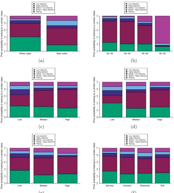
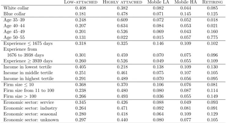
To visualize the main results, Figure 5 shows to which extent the prior probabilities of belonging to each of the five clusters are related to individual covariates; see also Table 4. For this evaluation, all other control variables are set to their mean values observed in the sample.
The prior probability that a worker with certain predetermined characteristics belongs to any cluster is computed for all MCMC draws and the reported values are the average over all the MCMC draws. The diagrams can, therefore, be interpreted as giving the prior probability that a worker belongs to one of these five clusters based solely on his known characteristics before plant closure.
A worker’s broad occupational status is highly related to group membership; see Figure 5, panel (a), as well as Table 4. Not surprisingly, white collar workers have a small prior probability to belong to Mobile + highly attached (4%). Most strikingly, blue collar workers have about half the risk of white collar workers to belong to Low-attached (18% versus 41%), which is a specific feature of plant closure events, see also Schwerdt et al. (2010).
With respect to age at the time of plant closure, we see in Figure 5, panel (b), as well as in Table 4 that all workers younger than 45 years have similar prior probabilities to belong to the various clusters. Not surprisingly, young workers have a low probability to belong to the Retiring cluster, but this probability strongly increases with age. While individuals with higher ages often belong to the Retiring cluster, their probability of being in Highly attached is reduced. For the oldest group, aged 50-55, the probability to be in the Retiring cluster is particularly high (77%), while the probability to belong to Highly attached is negligible.
The probability to belong to Mobile + highly attached is practically independent of age and the probability of belonging to Low-attached is slightly decreasing with age.
Work experience is less strongly related to group membership than age; see Figure 5, panel (c), and Table 4. We see that the five clusters are most evenly distributed among individuals with low levels of work experience. There is not much variation in cluster membership for individuals with low levels of experience, while at high levels of experience Highly attached and Mobile + low-attached dominate. In particular, higher experience levels are correlated with higher probability to belong to Highly attached and lower probability to belong to Mobile + low- attached . Interestingly, the probability of belonging to Retiring is practically independent of the amount of work experience. The pattern of distribution of cluster membership by tertiles of pre-displacement income resembles that of experience; see Figure 5, panel (d), and Table 4.
Figure 5, panel (e) and (f), as well as Table 4 show that group membership also varies with the size and industry affiliation of the firms from which workers are displaced. The groups with the largest Low-attached portion are workers from small firms and from the service sector.
The largest portion of the Mobile + highly attached cluster is exhibited by the workers of
medium size firms and workers from seasonal business outside of hotel and construction.
:KLWHFROODU %OXHFROODU 3ULRUSUREDELOLW\WREHORQJWRDFHUWDLQFODVV
/RZíDWWDFKHG +LJKO\DWWDFKHG 0RELOHORZíDWWDFKHG 0RELOHKLJKO\DWWDFKHG 5HWLULQJ
í í í í
3ULRUSUREDELOLW\WREHORQJWRDFHUWDLQFODVV
/RZíDWWDFKHG +LJKO\DWWDFKHG 0RELOHORZíDWWDFKHG 0RELOHKLJKO\DWWDFKHG 5HWLULQJ
(a) (b)
/RZ 0HGLDQ +LJK
3ULRUSUREDELOLW\WREHORQJWRDFHUWDLQFODVV
/RZíDWWDFKHG +LJKO\DWWDFKHG 0RELOHORZíDWWDFKHG 0RELOHKLJKO\DWWDFKHG 5HWLULQJ
/RZ 0HGLDQ +LJK
3ULRUSUREDELOLW\WREHORQJWRDFHUWDLQFODVV
/RZíDWWDFKHG +LJKO\DWWDFKHG 0RELOHORZíDWWDFKHG 0RELOHKLJKO\DWWDFKHG 5HWLULQJ
(c) (d)
/RZ 0HGLDQ +LJK
3ULRUSUREDELOLW\WREHORQJWRDFHUWDLQFODVV
/RZíDWWDFKHG +LJKO\DWWDFKHG 0RELOHORZíDWWDFKHG 0RELOHKLJKO\DWWDFKHG 5HWLULQJ
6HUYLFH ,QGXVWU\ 6HDVRQDO 1$
3ULRUSUREDELOLW\WREHORQJWRDFHUWDLQFODVV
/RZíDWWDFKHG +LJKO\DWWDFKHG 0RELOHORZíDWWDFKHG 0RELOHKLJKO\DWWDFKHG 5HWLULQJ
(e) (f)
Figure 5: Impact of each covariate on the prior probability of a worker to belong to a certain
cluster: (a) occupational state, (b) age, (c) experience, (d) income at time of plant closure, (e)
firm size, (f) firm’s economic sector (for each single covariate, all other covariates are set to their
mean values observed in the sample).
Low-attached Highly attached Mobile LA Mobile HA Retiring
White collar 0.408 0.382 0.082 0.044 0.085
Blue collar 0.181 0.478 0.071 0.145 0.125
Age 35–39 0.248 0.609 0.072 0.052 0.018
Age 40–44 0.207 0.634 0.084 0.053 0.021
Age 45–49 0.201 0.526 0.069 0.043 0.160
Age 50–55 0.131 0.022 0.015 0.057 0.775
Experience ≤ 1675 days 0.318 0.325 0.146 0.109 0.102
Experience from
1676 to 3938 days 0.301 0.459 0.070 0.075 0.096
Experience ≥ 3939 days 0.260 0.526 0.049 0.055 0.109
Income in lowest tertile 0.405 0.218 0.138 0.109 0.130
Income in middle tertile 0.251 0.461 0.075 0.107 0.105
Income in highest tertile 0.291 0.489 0.070 0.056 0.095
Firm size ≤ 10 0.368 0.370 0.106 0.076 0.081
Firm size from 11 to 100 0.238 0.480 0.080 0.087 0.114
Firm size > 100 0.266 0.493 0.036 0.055 0.149
Economic sector: service 0.345 0.426 0.088 0.049 0.093
Economic sector: industry 0.264 0.471 0.092 0.081 0.091
Economic sector: seasonal 0.280 0.418 0.064 0.109 0.129
Economic sector: unknown 0.297 0.440 0.080 0.077 0.105
Table 4: Displaced persons: Prior cluster probabilities for a single covariate. All other control variables are set to their mean values observed in the sample.
4.6 Comparison to the control group
After analyzing the career paths of displaced workers that are described by the five separate clusters, we turn to a comparison of the careers of displaced workers with a control group of workers not affected by a plant closure. This gives us some insights in the counterfactual situation that would have arisen if the plant closure had not taken place. To evaluate the counterfactual career trajectories for each cluster, we perform a posterior classification of controls based on the clustering model that was estimated for the displaced workers. In the following, we describe the corresponding classification of the controls and the simulation of the counterfactual career patterns in each cluster.
The selection of the control group as a weighted sample with similar pre-displacement char-
acteristics as the displaced group has been described in Section 2. The weighting procedure
ensures that displaced and controls are similar with respect to the covariates, which determine
prior group membership through the mixture-of-experts model specified in equation (4). The
only feature that distinguishes the two groups is the experience of a plant closure. It is evident
from Figure 3 that this shock has a dramatic effect on the state distribution π h of displaced
workers at the end of the first quarter, with a very high rate of being out of labor force for
practically all clusters. We thus have to take this event into account when simulating the career
trajectories of control group members.
Our main modelling assumption is that the state distribution π h at the end of the first quarter incorporates the entire effect of this shock. This means that the subsequent transition behaviour is independent from whether a person in this cluster experienced plant closure or not. The subsequent transition behaviour is characterized by the sequence of cluster-specific time-inhomogenous transition matrices ξ h = ( ξ h1 , . . . , ξ h,10 ) and the person’s given state at the end of the first quarter. While the typical career transitions are assumed to be the same for all persons within each cluster, regardless of whether the person experienced plant closure or not, it is to be expected that the state distribution at the end of the first quarter after (potential) plant closure is different for the displaced and the controls. Since the initial state y i0 is employment, i.e. y i0 = 1, also for all controls, the first transition of the controls is described by a row vector π c h = (π c h,1 , . . . , π h,4 c ) being different from π h and containing the probability distribution over all states at the end of the first quarter after plant closure for the controls. Our assumption implies that beyond the first quarter, the transition matrices ξ h1 , . . . , ξ h,10 , which were estimated from the displaced sample, can be used to classify the controls into the five clusters.
Based on this cluster model, the cluster assignment for control person i with observed individual time series denoted by y i c is performed by computing the posterior distribution t c ih ( θ 5 ) = Pr(S i c = h | y c i , θ 5 ) of the class indicator S i c over the 5 clusters by means of Bayes’
rule:
t c ih ( θ 5 ) ∝ p(y c i,−1 | y i1 c , ξ h )p(y i1 c | S i c = h, π c h )Pr(S i c = h |β 2 , . . . , β H , x c i ), h = 1, . . . , 5. (6) In (6), p(y i,−1 c | y c i1 , ξ h ) is the clustering kernel based on a time-inhomogeneous first order Markov chain as introduced in (2), whereas the cluster-specific state distribution π c h = (π c h,1 , . . . , π c h,4 ) for controls at the end of the first quarter after (potential) plant closure gives:
p(y c i1 | S i c = h, π c h ) = 4 k=1
π c h,k C i,k ,
with π h,k c = Pr(y c i1 = k | S i c = h) and C i,k = I { y i1 c = k } being an indicator for a non-displaced worker’s initial state. Pr(S i c = h |β 2 , . . . , β H , x c i ) is the prior class assignment distribution in- troduced in (4), which is based on the individual characteristics x c i of the control person under consideration.
Rather than estimating ( ξ 1 , . . . , ξ 5 , β 2 , . . . , β 5 ) again for the control panel, we use the MCMC draws obtained for the displaced persons to assign the individuals from the control panel to the five clusters of career patterns during an MCMC-type algorithm. Only the cluster-specific state distributions at the end of the first quarter are estimated by sampling π c h for each cluster from a Dirichlet distribution, π c h | S c , y ∼ D g 0,1 + C 1 h , . . . , g 0,4 + C 4 h
, where C k h =
i:S i =h C i,k is the total number of (non-displaced) workers in cluster h being in state k at the end of the first quarter after potential plant closure and π c h ∼ D (g 0,1 , . . . , g 0,4 ) follows a Dirichlet prior with hyperparameters analogous to those in Appendix A.
We assign individuals from the control panel using the posterior expectation ˆ t c ih = E(t c ih ( θ 5 ) | y c i ).
ˆ t c ih is estimated by evaluating and averaging t c ih ( θ 5 ) as given by (6) using the 15 000 MCMC
draws of ( ξ 1 , . . . , ξ 5 , β 2 , . . . , β 5 ) obtained for the panel of displaced workers and the 15 000
MCMC draws of π c h obtained for the panel of controls.
W W W W W W W W W W W W W
/R ZíDWWDFKHG
HPSOR\HG VLFN
RXWRIODERUIRUFH UHWLUHPHQW
W W W W W W W W W W W W W +LJKO\DWWDFKHG
W W W W W W W W W W W W W 0RELOHOR Z íDWWDFKHG
W W W W W W W W W W W W W 0RELOHKLJKO\DWWDFKHG
W W W W W W W W W W W W W
5HWLU LQJ
Figure 6: Posterior expectation of the distribution π c h,t over the 4 states (1 = employed, 2 = sick,
3 = out of labor force, 4 = retirement) after a period of t quarters in the various clusters (control
ííííí
/R ZíDWWDFKHG
íí
4XDUWHUW
/R ZíDWWDFKHG
HPSOR\HG VLFN RXWRIODERUIRUFH UHWLUHPHQW
ííííí
+LJKO\DWWDFKHG
íí
4XDUWHUW
+LJKO\DWWDFKHG
ííííí
0RELOHOR ZíDWWDFKHG
íí
4XDUWHUW
0RELOHOR ZíDWWDFKHG
ííííí
0RELOH+LJKO\$WWDFKHG
íí
4XDUWHUW
0RELOH+LJKO\$WWDFKHG
ííííí
5HWLU LQJ
íí