Weak convergence of a pseudo maximum likelihood estimator for the extremal index

SFB 823

Weak convergence of a

pseudo maximum likelihood estimator for the extremal index

Discussion Paper

Nr. 47/2016

ESTIMATOR FOR THE EXTREMAL INDEX

BETINA BERGHAUS AND AXEL B ¨UCHER

Abstract. The extremes of a stationary time series typically occur in clusters. A primary measure for this phenomenon is the extremal index, representing the recipro- cal of the expected cluster size. Both a disjoint and a sliding blocks estimator for the extremal index are analyzed in detail. In contrast to many competitors, the estima- tors only depend on the choice of one parameter sequence. We derive an asymptotic expansion, prove asymptotic normality and show consistency of an estimator for the asymptotic variance. Explicit calculations in certain models and a finite-sample Monte Carlo simulation study reveal that the sliding blocks estimator is outperforming other blocks estimators, and that it is competitive to runs- and inter-exceedance estimators in various models. The methods are applied to a variety of financial time series.

Key words. Clusters of extremes, extremal index, stationary time series, mixing coefficients, block maxima.

1. Introduction

An adequate description of the extremal behavior of a time series is important in many applications, such as in hydrology, finance or actuarial science (see, e.g., Section 1.3 in the monograph Beirlant et al., 2004). The extremal behavior can be characterized by the tail of the marginal law of the time series and by the serial dependence; that is, by the tendency that extremal observations tend to occur in clusters. A primary measure of extremal serial dependence is given by the extremal index θ ∈ [0,1], which can be interpreted as being equal to the reciprocal of the mean cluster size. The underlying theory was worked out in Leadbetter (1983); Leadbetter et al. (1983); O’Brien (1987);

Hsing et al. (1988);Leadbetter and Rootz´en (1988).

Estimating the extremal index based on a finite stretch from the time series has been extensively studied in the literature. Common approaches are based on the blocks method, the runs method and the inter-exceedance times method (see Beirlant et al., 2004, Section 10.3.4, for an overview). The first two methods usually depend on two parameters to be chosen by the statistician: a threshold sequence and a cluster iden- tification scheme parameter (such as a block length). In contrast, inter-exceedance type-estimators are attractive since they only depend on a threshold sequence. Some references are Hsing(1993);Smith and Weissman (1994); Weissman and Novak(1998);

Ferro and Segers(2003);S¨uveges(2007);Robert(2009);Robert et al.(2009), among oth- ers. The present paper is on a slight modification of a blocks estimator due toNorthrop (2015), which, remarkably, only depends on a cluster identification parameter. This makes the estimator practically appealing in comparison to other blocks methods.

Date: August 5, 2016.

1

In many papers on estimating the extremal index, either no asymptotic theory is given (such as inS¨uveges,2007;Northrop,2015), or the asymptotic theory is incomplete in the sense that theory is developed for a non-random threshold sequence, while in practice a random sequence must be used (as, e.g., in Weissman and Novak, 1998;

Robert et al., 2009). As pointed out in the latter paper, “the mathematical treatment of such random threshold sequences requires complicated empirical process theory”. In the present paper, the mathematical treatment is comprehensive, working out all the arguments needed from empirical process theory.

Let us proceed by motivating and defining the estimator: throughout, X1, X2, . . . denotes a stationary sequence of real-valued random variables with stationary cumulative distribution function (cdf)F. The sequence is assumed to have an extremal indexθ ∈ (0,1]: for anyτ >0, there exists a sequence un=un(τ) such that limn→∞nF¯(un) =τ and such that

n→∞lim P(M_1:n≤u_n) =e^−θτ. (1.1) Here, ¯F = 1−F and M_1:n= max(X₁, . . . , X_n).

For simplicity, we assume that F is continuous and define a sequence of standard uniform random variables byU_s =F(X_s). Forx∈(0,1), letu_n=F^←(x^1/n), whereF^← denotes the generalized inverse of the cdfF. ThennF¯(un) =n(1−x^1/n)→ −log(x) as n→ ∞ and therefore, by (1.1)

P(N_1:nⁿ ≤x) =P(M_1:n≤u_n)→e^θlogx=x^θ, (1.2) whereN_1:n=F(M_1:n) = max{U₁, . . . , U_n}. In other words,N_1:nⁿ asymptotically follows a beta-distribution with parameters (θ,1), inspiringNorthrop(2015) to estimateθby the maximum likelihood estimator for the beta-distribution, based on a sample of estimated block maxima (see below). A slight modification of this estimator can be worked out by considering a further transformation toZ1:n=n(1−N1:n). Equation (1.2) immediately implies that

P(Z_1:n≥x) =P(N_1:nⁿ ≤ {1−x/n}ⁿ)→exp(−θx), n→ ∞, (1.3) that is,Z_1:n asymptotically follows the exponential distribution with parameter θ.

Now suppose that we observe a stretch of length n from the time series (Xs)s≥1. Divide the sample into k_n blocks of length b_n, and for simplicity assume that n=b_nk_n (otherwise, the final block would consist of less than b_n observations and should be omitted). Fori= 1, . . . , kn, let

Mni=M_{((i−1)bn+1):(ibn)}= max{X_(i−1)bn+1, . . . , X_ibn}

denote the maximum over the Xs from the ith block. Also, let Nni = F(Mni) = max{U_(i−1)bn+1, . . . , U_ibn}andZni =bn(1−N_ni). Ifbnis sufficiently large, then, by (1.3), the (unobservable) random variablesZ_n1, . . . , Z_nk form an approximate sample from the Exponential(θ)-distribution. Moreover, as common when working with block maxima of a time series, they may be considered as asymptotically independent, which suggests to estimateθ by the maximum-likelihood estimator for the Exponential(θ) distribution:

θ˜n= 1

k_n

kn

X

i=1

Zni

−1

.

Note that ˜θ_n should not be considered an estimator, as it is based on the unknown cdf F. Subsequently, we call ˜θ_n an oracle forθ.

In practice, the Us are not observable, whence they need to be replaced by their observable counterparts giving rise to the definitions

Nˆ_ni= ˆF_n(M_ni) and Zˆ_ni=b_n(1−Nˆ_ni), where ˆFn(x) =n⁻¹Pn

s=11(Xs ≤x) denotes the empirical cdf ofX1, . . . , Xn. We obtain the estimator

θˆn= ˆθ_n^dj= 1 k_n

kn

X

i=1

Zˆni

−1

, (1.4)

which is, up to an error of ordero_P(k^−1/2_n ), equal to the estimator{−_k¹

n

Pkn

i=1log( ˆN_ni^bn)}⁻¹ considered in Northrop (2015) (where no asymptotic theory is given). While deriving the asymptotic distribution of the oracle ˜θ_n may appear tractable (essentially, a cen- tral limit theorem for rowwise dependent triangular arrays is to be shown, followed by an argument using the delta method), asymptotic theory on the estimator ˆθn is sub- stantially more difficult due to the additional serial dependence induced by the rank transformation (which on top of that operates between blocks instead of within blocks).

A central contribution of the present paper is the derivation of the asymptotic distri- bution of ˆθn. It will turn out that the impact of the rank transformation is non-negligible, resulting in different asymptotic variances of ˆθn and the corresponding oracle ˜θn. We also present asymptotic theory for a modification of ˆθ_n based on sliding block maxima.

The asymptotic expansions derived in this paper also suggest an estimator for the as- ymptotic variance of ˆθ_n, which is the second main contribution. A third contribution consists of a bias reduction method to improve the finite-sample approximation.

The remaining parts of this paper are organized as follows: in Section 2, we present mathematical preliminaries needed to formulate and derive the asymptotic distributions of the estimators forθ. Consistency and asymptotic normality is then shown in Section3.

In Section4, we propose a simple device to reduce the bias of the estimators. Estimators of the asymptotic variance are handled in Section 5. Examples are worked out in detail in Section6, while finite-sample results and a case study are presented in Section7and8, respectively. The complete proof of the main result for the disjoint blocks estimator is given is Section 9, and additional proofs are postponed to a supplementary material (Appendices A andB).

2. Mathematical preliminaries

The serial dependence of the time series (X_s)_swill be controlled via mixing coefficients.

For two sigma-fields F₁,F₂ on a probability space (Ω,F,P), let α(F₁,F₂) = sup

A∈F₁,B∈F₂

|P(A∩B)−P(A)P(B)|.

In time series extremes, one usually imposes assumptions on the decay of the mixing coefficients between sigma-fields generated by {X_i1(X_s > F^←(1−ε_n)) : s ≤ `} and {X<sub>s</sub>1(Xs > F<sup>←</sup>(1−εn)) : s ≥ `+k}, where εn → 0 is some sequence reflecting the fact that only the dependence in the tail needs to be restricted (see, e.g., Rootz´en,

2009). For our purposes, we need slightly more to control even the dependence between the smallest of all block maxima (see also Condition 2.1(v) below). More precisely, for −∞ ≤ p < q ≤ ∞ and ε ∈ (0,1], let B^ε_p:q denote the sigma algebra generated by U_s^ε:=U_s1(U_s>1−ε) withs∈ {p, . . . , q}and define, for `≥1,

αε(`) = sup

k∈N

α(B^ε_1:k,B_k+`:∞^ε )

Note that the coefficients are increasing inε, whence they are bounded by the standard alpha-mixing coefficients of the sequenceUs, which can be retrieved for ε= 1. In Con- dition2.1(iii) below, we will impose a condition on the decay of the mixing coefficients for small values ofε.

The extremes of a time series may be conveniently described by the point process of normalized exceedances. The latter is defined, for a Borel set A ⊂ E := (0,1] and a numberx∈[0,∞), by

N_n^(x)(A) =

n

X

s=1

1(s/n∈A, Us>1−x/n).

Note that Nn^(x)(E) = 0 iff N1:n ≤1−x/n; the probability of that event converging to e^−θx under the assumption of the existence of extremal indexθ.

Fix m ≥ 1 and x1 > · · · > xm > 0. For 1 ≤ p < q ≤ n, let F_p:q,n^(x1,...,xm) denote the sigma-algebra generated by the events {U_i >1−x_j/n} forp ≤ i≤q and 1 ≤j ≤ m.

For 1≤`≤n, define

α_n,`(x₁, . . . , x_m) = sup{|P(A∩B)−P(A)P(B)|:

A∈ F_1:s,n^(x1,...,xm), B∈ F<sub>s+`:n,n</sub><sup>(x1,...,xm)</sup>,1≤s≤n−`}.

The condition ∆_n({u_n(x_j)}_1≤j≤m) is said to hold if there exists a sequence (`_n)_n with

`n = o(n) such that αn,`n(x1, . . . , xm) = o(1) as n → ∞. A sequence (q_n)n with qn = o(n) is said to be ∆n({u_n(xj)}_1≤j≤m)-separating if there exists a sequence (`n)n with

`n=o(qn) such that nq<sub>n</sub><sup>−1</sup>α<sub>n,`n</sub>(x1, . . . , xm) =o(1) as n→ ∞. If ∆_n({u_n(xj)}_1≤j≤m) is met, then such a sequence always exists, simply take q_n=bmax{nα^1/2_n,`

n,(n`_n)^1/2}c.

By Theorems 4.1 and 4.2 in Hsing et al. (1988), if the extremal index exists and the ∆(un(x))-condition is met (m = 1), then a necessary and sufficient condition for weak convergence ofNn^(x) is convergence of the conditional distribution ofNn^(x)(Bn) with B_n= (0, q_n/n] given that there is at least one exceedance of 1−x/n in{1, . . . , q_n} to a probability distribution π on N, that is,

n→∞lim P(N_n^(x)(B_n) =j|N_n^(x)(B_n)>0) =π(j) ∀j≥1,

whereqnis some ∆(un(x))-separating sequence. Moreover, in that case, the convergence in the last display holds for any ∆(u_n(x))-separating sequence q_n. If the ∆(u_n(x))- condition holds for any x > 0, thenπ does not depend on x (Hsing et al., 1988, Theo- rem 5.1).

A multivariate version of the latter results is stated in Perfekt (1994), see also the summary in Robert (2009), page 278, and the thesis Hsing (1984). Suppose that the extremal index exists and that the ∆(u_n(x₁), u_n(x₂))-condition is met for any x₁ ≥

x₂ ≥ 0, x₁ 6= 0. Moreover assume that there exists a family of probability measures {π^(σ)₂ :σ∈[0,1]}on J ={(i, j) :i≥j≥0, i≥1} such that

n→∞lim P(N_n^(x1)(Bn) =i, N_n^(x2)(Bn) =j|N_n^(x1)(Bn)>0) =π₂^(x2/x1)(i, j) ∀(i, j)∈ J, where q_n is some ∆(u_n(x₁), u_n(x₂))-separating sequence. In that case, the two-level point process Nn^(x1,x2)= (Nn^(x1), Nn^(x2)) converges in distribution to a point process with characterizing Laplace transform explicitly stated in Robert(2009) on top of page 278.

Note that

π₂⁽¹⁾(i, j) =π(i)1(i=j), π₂⁽⁰⁾(i, j) =π(i)1(j= 0).

The following set of conditions will be imposed to establish asymptotic normality of the estimators.

Condition 2.1.

(i) Extremal index and the point process of exceedances. The extremal index θ ∈ (0,1] exists and the above assumptions guaranteeing convergence of the one- and two-level point process of exceedances are satisfied.

(ii) Moment assumption on the point process. There existsδ >0 such that, for any ` >0, there exists a constantC<sub>`</sub>⁰ such that

E[|N_n^(x1)(E)−N_n^(x2)(E)|^2+δ]≤C<sub>`</sub><sup>0</sup>(x1−x2) ∀`≥x1 ≥x2≥0.

(iii) Asymptotic independence in the big-block/small-block heuristics. There existsc2 ∈(0,1) and C2>0 such that

αc2(`)≤C2`^−η

for some η ≥3(2 +δ)/(δ−µ) >3 with 0 < µ < δ∧(1/2) and with δ >0 from Condition (ii). The block sizeb_n→ ∞ is chosen in such a way that

kn=o(b²_n), n→ ∞, (2.1)

and such that there exists a sequence `_n → ∞ (to be thought of as the length of small blocks which are to be clipped-of at the end of each block of sizebn) satisfying

`<sub>n</sub>=o(b<sup>2/(2+δ)</sup><sub>n</sub> ), k<sub>n</sub>α<sub>c2</sub>(`_n) =o(1);

all convergences being for n→ ∞.

(iv) Bound on the variance of the empirical process. There exist some constants c₁ ∈(0,1), C₁>0 such that, for ally∈(0, c₁) and all n∈N,

VarnXⁿ

s=1

1(U_s>1−y)o

≤C₁(ny+n²y²).

(v) All standardized block maxima of sizeb_n/2converge to 1. For allc∈(0,1), we have

n→∞lim P _2k

minn

i=1 N_ni⁰ ≤c

= 0,

where N_ni⁰ = max{U_s :s∈[(i−1)bn/2 + 1, . . . , ibn/2]}, for i= 1, . . . ,2kn, denote consecutive standardized block maxima of (approximate) sizeb_n/2.

(vi) Existence of moments of maxima. Withδ >0 from Condition (ii), we have lim sup

n→∞ E[Z_1:n^2+δ]<∞.

(vii) Bias. As n→ ∞,

E[Z_1:bn] =θ⁻¹+o(k_n^−1/2).

Assumptions (i)–(iii) are suitable adaptations of Conditions (C1) and (C2) inRobert (2009); in fact, they can be seen to imply the latter. Among other things, these conditions are needed to apply his central result, Theorem 4.1, on the weak convergence of the tail empirical process on [0,∞). Note that the assumptions are satisfied for solutions of stochastic difference equations, see Example 3.1 in Robert (2009). The Assumption in (2.1) is a growth condition that is needed in the proof of Lemma 9.1. As argued in Robert et al.(2009), it is actually a weak requirement, as in many time series models it is a necessary condition for the bias condition in (vii) to be true (see Section6 below).

Finally, a positive extremal index can be guaranteed by assuming that

m→∞lim lim sup

n→∞ P(N_m:bn >1−^x_n |U₁ ≥1−^x_n) = 0 (2.2) for anyx >0, seeBeirlant et al. (2004), formula (10.8). We will additionally need this assumption for the calculation of the asymptotic variance of the estimators.

In a slightly different form concerning only the tail, Assumption (iv) has also been made in Condition (C3) inDrees(2000) for proving weak convergence of the tail empirical process. In comparison to there, the extra factor n²y² allows for additional flexibility, in that it allows forO(n²)-non-negligible covariances, as long as their contribution is at most y². In Section 6, we show that the assumption holds for solutions of stochastic difference equations, such as the ARCH-model, and for max-autoregressive models.

Recall that N_ni^bn is approximately Beta(θ,1)-distributed. As a consequence, every standardized block maximumNnimust converge to 1 as the sample size grows to infinity.

Still, out of the sample ofk_n block maxima, the smallest one could possibly be smaller than one, especially when the number of blocks is large. Assumption (v) prevents this from happening; note that a similar assumption has also been made inB¨ucher and Segers (2015), Condition 3.2. Imposing the assumption even for block maximaN_ni⁰ of sizebn/2 guarantees that also the minimum over all big sub-block maxima (needed in the proof for the disjoint blocks estimator) and the minimum over all sliding block maxima of size bn (needed in the proof for the sliding blocks estimator) converges to 1.

Assumption (vi) is needed to deduce uniform integrability of the sequence Z_1:b²

n. It implies convergence of the variance ofZ1:bn to that of an exponential distribution with parameter θ. Finally, (vii) requires the approximation of the first moment of Z_1:bn by that of an exponential distribution to be sufficiently accurate.

3. Main results

In this section we prove consistency and asymptotic normality of the disjoint blocks estimator ˆθ^djn defined in (1.4), as well as of a variant which is based on sliding blocks and which we will denote by ˆθ^sl_n. We begin by defining the latter estimator.

Divide the sample inton−b_n+ 1 blocks of lengthb_n, i.e., fort= 1, . . . , n−b_n+ 1, let M_nt^sl =M_t:(t+bn−1)= max{X_t, . . . , X_t+bn−1}.

Analogously to the notation used in the definition of the estimator for disjoint blocks, we will write N_nt^sl =F(M_nt^sl) and Z_nt^sl =bn(1−N_nt^sl) and define their empirical counterparts Nˆ_nt^sl = ˆFn(M_nt^sl) and ˆZ_nt^sl = bn(1−Nˆ_nt^sl), where ˆFn is the empirical cdf of X1, . . . , Xn. Just as for the disjoint blocks estimator, the (pseudo-)observations ˆZ_nt^sl are approximately exponentially distributed with meanθ⁻¹, which suggests to estimateθby the reciprocal of their empirical mean, i.e.,

θˆ^sl_n = 1 n−bn+ 1

n−b_n+1

X

t=1

Zˆ_nt^sl

!⁻¹ .

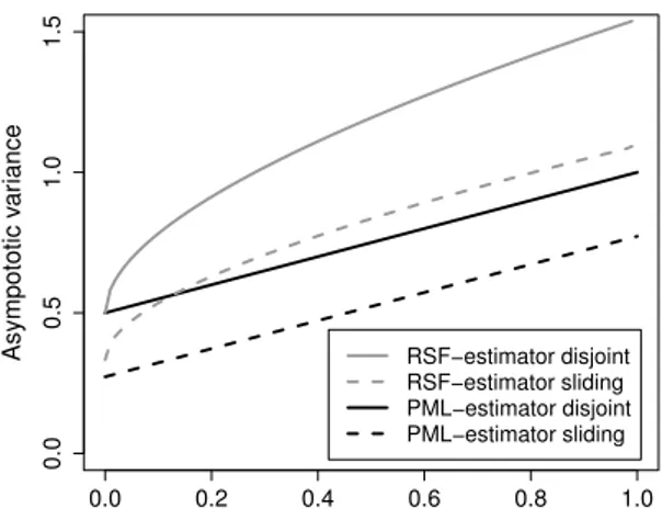
Note that no data has to be discarded ifbnis not a divisor of the sample sizen. While ˆθ_n^sl is based on a substantially larger number of blocks than the disjoint blocks estimator, the blocks are heavily correlated. The following theorem is the central result of this paper and shows that both estimators are consistent and converge at the same rate to a normal distribution. The disjoint blocks estimator has a larger asymptotic variance than the sliding blocks estimator.

Theorem 3.1. Suppose that Condition 2.1 and (2.2) is met. Then pk_n(ˆθ^dj_n −θ) N(0, θ⁴σ_dj²) and p

k_n(ˆθ^sl_n−θ) N(0, θ⁴σ²_sl), where

σ²_dj= 4 Z 1

0

E[ζ₁^(σ)ζ₂^(σ)]

(1 +σ)³ dσ+ 4θ⁻¹ Z 1

0

E[ζ₁^(σ)1(ζ₂^(σ)= 0)]

(1 +σ)³ dσ−θ⁻², σ_sl² = 4

Z 1 0

E[ζ₁^(σ)ζ₂^(σ)]

(1 +σ)³ dσ+ 4θ⁻¹ Z 1

0

E[ζ₁^(σ)1(ζ₂^(σ)= 0)]

(1 +σ)³ dσ− 4−4 log(2) θ² , with (ζ₁^(σ), ζ₂^(σ))∼π^(σ)₂ . In particular,σ²_dj=σ²_sl+{3−4 log(2)}/θ²≈σ²_sl+ 0.2274/θ².

It is interesting to note that the asymptotic variance of the disjoint blocks estimator is substantially more complicated than if one would naively treat theZ_ni as an iid sample from the exponential distribution with parameter θ (as is done in Northrop, 2015; the variance would then simply beθ²). A heuristic explanation can be found in Remark3.3 below. A formal proof is given at the end of this section, with several auxiliary lemmas postponed to Section 9 (for the disjoint blocks estimator) and to Appendix A in the supplement (for the sliding blocks estimator). Explicit calculations are possible for instance for a max-autoregressive process, see Section 6.1, or for the iid case.

Example 3.2. If the time series is serially independent, a simple calculation shows that π(i) =1(i= 1) andπ^(σ)₂ (i, j) = (1−σ)1(i= 1, j = 0) +σ1(i= 1, j= 1). This implies

θ= 1, E[ζ₁^(σ)ζ₂^(σ)] =σ, E[ζ₁^(σ)1(ζ₂^(σ)= 0)] = 1−σ

and therefore θ⁴σ_dj² = 1/2 and θ⁴σ_sl² ≈0.2726. It is worthwhile to mention that these values are smaller than the variances of any of the disjoint and sliding blocks estimators considered inRobert et al.(2009), respectively. Moreover, it can be seen that the same formulas are valid wheneverθ= 1: the fact thatθ⁻¹ ≥P∞

i=1iπ(i) implies thatπ(1) = 1.

By (9.9), we then obtain π₂^(σ) = (1−σ)1(i= 1, j= 0) +σ1(i= 1, j = 1).

Remark 3.3 (Main idea for the proof). Define Tˆ_n^dj= 1

k_n

kn

X

i=1

Zˆni, T_n^dj= 1

k_n

kn

X

i=1

Zni. (3.1)

Tˆ_n^sl= 1 n−b_n+ 1

n−bn+1

X

t=1

Zˆ_nt^sl, T_n^sl= 1 n−b_n+ 1

n−bn+1

X

t=1

Z_nt^sl. (3.2) In the following, we only consider the disjoint blocks estimator, the argumentation for the sliding blocks estimator is similar. For the ease of notation, we will skip the upper index and just write ˆTninstead of ˆTn^dj, etc. Asympotic normality of ˆθnmay be deduced from the delta method and weak convergence of√

k( ˆTn−θ⁻¹). The roadmap to handle the latter is as follows: decompose

pk_n( ˆT_n−θ⁻¹) =p

k_n( ˆT_n−T_n) +p

k_n(T_n−θ⁻¹). (3.3) Using a big-block/small-block type argument, the asymptotics of the second summand on the right-hand side can be deduced from a central limit theorem for rowwise independent triangular arrays. Depending on the choice of the block sizes, an asymptotic bias term may appear, which we control by Condition2.1(vii). The first summand is more involved, and also contributes to the limiting distribution: first, for x≥0, let

e_n(x) = 1

√kn n

X

s=1

{1(U_s >1−x/b_n)−x/b_n} (3.4) denote the tail empirical process ofX1, . . . , Xn and let

Hˆkn(x) = 1 kn

kn

X

i=1

1(Zni≤x) (3.5)

be the empirical distribution function ofZ_n1, . . . , Z_nkn. Then pk_n( ˆT_n−T_n) = bn

√k_n

kn

X

i=1

(N_ni−Nˆ_ni) = bn

n√ k_n

kn

X

i=1 n

X

s=1

{N_ni−1(U_s≤N_ni)} (3.6)

= 1

kn^3/2 kn

X

i=1 n

X

s=1

{1(U_s>1−Z_ni/b_n)−Z_ni/b_n}

= 1 k_n

kn

X

i=1

e_n(Z_ni) =

Z max^kn_i=1Zni

0

e_n(x) d ˆH_kn(x).

SinceZni is approximately exponentially distributed with parameterθ, one may expect that ˆH_kn(x) converges to H(x) = 1−exp(−θx) in probability, for n→ ∞ and for any x≥0. Moreover, on an appropriate domain,e_n efor some Gaussian processe(Drees, 2000,2002;Rootz´en,2009;Robert,2009;Drees and Rootz´en,2010), whence a candidate limit for the expression on the left-hand side of the previous display is given by

Z ∞ 0

e(x)θe^−θxdx.

The latter distribution is normal, and joint convergence of both terms on the right-hand side of (3.3) will finally allow for the derivation of the asymptotic distribution of ˆθ_n. These heuristic arguments have to be made rigorous.

Proof of Theorem 3.1 (Disjoint blocks). Write ˆT_n = ˆT_n^dj and T_n =T_n^dj. Recall the defi- nitions of en and ˆHkn in (3.4) and (3.5), respectively. For `∈N, let

D_n=

Z maxZni

0

e_n(x) d ˆH_kn(x), D<sub>n,`</sub> = Z `

0

e_n(x) d ˆH_kn(x), D<sub>`</sub> = Z `

0

e(x)θe^−θxdx.

Also, let G_n=√

k_n(T_n−ET_n) and letGbe defined as in Lemma9.3. Suppose we have shown that

(i) For all δ >0: lim`→∞lim sup<sub>n→∞</sub>P(|D<sub>n,`</sub>−D_n|> δ) = 0;

(ii) For all `∈N: D<sub>n,`</sub>+Gn D_`+Gas n→ ∞;

(iii) D<sub>`</sub>+G D+G∼ N(0, σ<sub>dj</sub><sup>2</sup>) as `→ ∞.

It then follows from (3.6) and Wichura’s theorem (Billingsley,1979, Theorem 25.5) that

√n( ˆT_n−ET_n) =D_n+G_n N(0, σ_dj²), n→ ∞.

By Condition 2.1(vii), we obtain that √

kn( ˆTn−θ⁻¹) N(0, σ²_dj). The theorem then follows from the delta-method.

The assertion in (i) is proved in Lemma 9.1. The assertion in (ii) is proved in Lemma 9.5. The assertion in (iii) follows from the fact that D_{`</sub> +G is normally dis- tributed with variance σ<sub>`}² as specified in Lemma 9.5, and the fact that by Lemma 9.6

σ²<sub>`</sub> →σ<sub>dj</sub><sup>2</sup> for`→ ∞.

Proof of Theorem 3.1 (Sliding blocks). Let ˆH_k^sl

n denote the empirical distribution func- tion of the Z_nt^sl, i.e., ˆH_k^sl_n(x) = _n−b¹

n+1

Pn−bn+1

t=1 1(Z_nt^sl ≤x) and let D_n^sl=

Z maxtZ^sl_nt 0

en(x) d ˆH_k^sl_n(x), D^sl<sub>n,`</sub> = Z `

0

en(x) d ˆH_k^sl_n(x), D^sl<sub>`</sub> = Z `

0

e(x)θe^−θxdx.

With this notation the proof follows along the same lines as for the disjoint blocks, with Lemma 9.1,9.2 and 9.3replaced by Lemma A.1,A.2and A.3, respectively.

4. Bias reduction

Throughout this section, let ( ˆT_n, T_n)∈ {( ˆTn^dj, Tn^dj),( ˆT_n^sl, T_n^sl)}denote any of the quan- tities defined in (3.1) or (3.2). A Taylor expansion allows to approximately decompose the bias of the estimator ˆθn= ˆT_n⁻¹ into two parts:

µ_n= E[ ˆT_n⁻¹−θ]≈ −θ²E[ ˆT_n−θ⁻¹] =−θ²E[ ˆT_n−T_n]−θ²E[T_n−θ⁻¹] =:µ_n1+µ_n2. The second component µ_n2 is inherent to the time series (X_s)s∈N itself. In many ex- amples, it can be seen to be of the order O(b⁻¹_n ), see for instance Section 6 or similar calculations made in (Robert et al., 2009, Section 6). The first component µn1 is es- sentially due to the use of the empirical distribution function in the definition of the estimator. The following lemma gives a first-order asymptotic expansion, which turns out to be the same for the disjoint and sliding blocks estimator.