Using the extremal index for value-at-risk backtesting

SFB 823

Using the extremal index for value-at-risk backtesting

Discussion Paper Axel Bücher, Peter N. Posch,

Philipp Schmidtke

Nr. 25/2018

Using the Extremal Index for Value-At-Risk Backtesting

Axel B¨ ucher

, Peter N Posch

, Philipp Schmidtke

First version: Sept 2017. This version: October 15, 2018

Abstract

We introduce a set of new Value-at-Risk independence backtests by establishing a connection between the independence property of Value-at-Risk forecasts and the extremal index, a general measure of extremal clustering of stationary sequences.

We introduce a sequence of relative excess returns whose extremal index has to be estimated. We compare our backtest to both popular and recent competitors using Monte-Carlo simulations and find considerable power in many scenarios.

In an applied section we perform realistic out-of-sample forecasts with common forecasting models and discuss advantages and pitfalls of our approach.

Key words: VaR Backtesting, Extremal Index, Independence, Risk measures.

JEL Classification: C52, C53, C58.

∗Heinrich Heine University D¨usseldorf, Mathematical Institute, Universit¨atsstr. 1, 40225 D¨usseldorf, Germany

†TU Dortmund University, Chair of Finance, Otto-Hahn-Str. 6, 44227 Dortmund, Germany

‡TU Dortmund University, Chair of Finance, Otto-Hahn-Str. 6, 44227 Dortmund, Germany, E-Mail: philipp.schmidtke@udo.edu. Corresponding author.

1 Introduction

In spite of its usage as a risk measure for more than 20 years, researchers are still engaged in exploring new forecasting and backtesting procedures for the Value-at- Risk (VaR). The latter procedures are typically based on a statistical test which tries to assess whether a certain desirable property is met for the observed sequence of VaR-violations: first, the concept of correct unconditional coverage aims at checking whether the number of overall violations is justifiable. From an academic perspective, we typically seek for a forecasting procedure which yields neither too many nor too few violations. On the other hand, regulators are usually interested in situations where the risk is not underestimated, resulting in a focus on not too many violations. Second, thecorrect independence aspect focuses on possible serial dependence of violations, and aims at checking whether the sequence of violations behaves like an independent sequence. This concept becomes most important if unconditional coverage is statistically satisfied, i.e., an unconditional test cannot be rejected. In that case, a test using information about the way how violations occur has still potential to reject the forecasts. Available independence backtests may have power only with respect to a lack of independence, or with respect to both the lack of independence and of correct unconditional coverage. The latter ones are called conditional coverage tests.

In general, tackling the independence property is challenging. This is mainly due to the fact that risk forecasts deal with low probability events and an often short testing sample. As a consequence, observing many violations is unlikely, which naturally results in small effective sample sizes and, therefore, bad power properties. In addition, some of the classical tests explicitly assume an alternative model incorporating a special kind of dependence, which may also result in a loss of power if in fact a more general form of dependence is present.

As a matter of fact, most financial time series exhibit large degrees of heteroscedas- ticity and therefore require for time-changing risk forecasts. Renouncement would lead to a probably threatening violation clustering, something a sound risk man- agement should always aim to prevent.

We contribute to the backtesting literature by introducing a new test for the independence hypothesis which is particularly sensitive to deviations from indepen- dence among the most extreme observations. Unlike standard methods, the new test does not use solely the 0-1-violation sequence. Instead, we assess whether a series of VaR-adjusted returns, coinedrelative excess returns, exhibits a significant tendency for that its most extreme observations occur in clusters. As a measure for that tendency, we employ the extremal index, a natural measure of clustering of extreme observations stemming from extreme value theory. We implement the approach with two different extremal index estimators, the first one (S¨uveges and Davison, 2010) leading to a more classic 0-1-test, while the second one (Northrop, 2015; Berghaus and B¨ucher, 2017) enables the processing of more detailed infor- mation. We find considerable power improvements in many cases in comparison to common competing tests, with the second test often showing the most convincing results.

As is well known, VaR lacks some important features of risk measures. The most common alternative measure is provided by the Expected Shortfall (ES), which will soon replace the VaR as the standard regulatory measure of risk for banks (BCBS, 2016). However, since VaR and ES are closely related, it does not come as a surprise that VaR and its backtests also play a prominent role in some ES backtests. For example, Kratz et al. (2018) propose a joint backtest for several VaR levels as an intuitive way to implicitly backtest ES. A second example is BCBS (2016) itself, where out-of-sample backtesting is based on VaR as well. However, both in general and in the aforementioned examples, the issue of a possible lack of

independence is rarely addressed. Since the implementation of our idea is relatively independent of the specific VaR level, we see this as a promising approach in this respect.

The remainder of this paper is structured as follows. Section 2 provides prelim- inaries about the notation, a more detailed description of the backtesting problem alongside with a short overview of existing tests, and mathematical details on the extremal index. Section 3 introduces our new approach of independence backtest- ing based on the extremal index. In Section 4, we perform a detailed analysis of the small-sample properties, while Section 5 focuses on some empirical implica- tions. Finally, Section 6 concludes, while less important aspects are deferred to a sequence of appendices.

2 Preliminaries on Backtesting and the Extremal Index

In this section we review the essentials of VaR backtesting and introduce our notation. Then we turn to the extremal index and its estimators.

2.1 Backtesting the Value-at-Risk

Consider a random return r_t of a financial asset in a period t, usually a day.

Suppose this return is continuously distributed with c.d.f. Ft, conditional on the information setFt−1 which embodies all information up to periodt−1. We define the Value-at-Risk at levelp as VaR^(t)_p :=−F_t⁻¹(p), where F_t⁻¹ denotes the inverse of F_t. Throughout the paper, we will refer to pas VaR level, usual values are 5 % and 1 %, whereas q = 1−p will be called the VaR confidence level. Note that, with this definition, we report large losses and hence VaRs as positive numbers.

A violation at time t occurs if r_t < −VaRd^(t)_p , where VaRd^(t)_p denotes a forecast of the true VaR at period t, calculated based on information from Ft−1. Using a series of VaR forecasts corresponding to observed returnsr₁, . . . , r_n, we define the violation sequence (I_t)ⁿ_t=1, by

I_t =







1 (violation), if rt<−VaRd^(t)_p 0 (compliance), if rt≥ −VaRd^(t)_p

. (2.1)

The time points t where violations occur, that is I_t= 1, are called violation times or violations indices. Suppose there are M1 violations, that is, M1 = #{It = 1}, and order the violation times increasingly t₁ < · · · < t_M1. We define the inter- violation durations Di as Di := ti+1 −ti, where i = 1, . . . , M1 −1. If the VaR forecasts happen to be completely correct, that is VaRd^(t)_p = VaR^(t)_p for all t, then the violation sequence forms an i.i.d. Bernoulli sequence with success probability p, that is I_t ^i.i.d.∼ Bernoulli(p). This implies M₁ = Pn

t=1I_t ∼ Binom(n, p) and Di

i.i.d.

∼ Geom(p).

The goal of backtesting is to asses whether a sequence of n ex-ante VaR fore- casts are appropriate in relation to the realized returns. This is usually done by stressing one of the above mentioned properties of the violation sequence or the durations.

Since Christoffersen (1998) backtests are classified according to their focus, see also the discussion in the introduction. The property of forecasts being completely unsuspicious is called correct conditional coverage (cc) and may be written as

cc: I_t^i.i.d.∼ Bernoulli(p), t= 1, . . . , n. (2.2) Before this term was introduced, assessing VaR forecasts was solely concerned with the aspect ofunconditional coverage (uc) which is defined by

uc: E(I_t) = p, t = 1, . . . , n. (2.3)

In other words, uc is concerned about whether the frequency of violations is rea- sonable in the sense that, for all time points t, the probability of observing an violation equals p, which is the probability had the true VaR been used for the calculation ofIt. A simple way to get a first impression about the latter property is to calculate the actual number of violations M₁ and compare the result to its expectationnpunder the assumptionVaRd^(t)_p = VaR^(t)_p . See, e.g., Kupiec (1995) for an early test or BCBS (1996b) for the Traffic Light Approach used by the Basel Committee.

Unconditional coverage is complemented by the independence property (ind), given by

ind: I₁, . . . , I_n are stochastically independent. (2.4) Rather than on how many violations occur, the focus is on how the violations occur over time. A simple graphical way to check this property is to look on a plot of VaR violations and assess visually whether there are any patterns. However, detecting a failure of the independence property can be fairly hard due to the natural scarcity of violations if the VaR level is sufficiently small or the backtesting sample is not large enough. Still, possible dependence among violations can be extremely important for risk managers, as subsequent violations can sum up and result in an overall loss of threatening magnitude.

Note that, from a more technical perspective, plain independence of violations does not necessarily imply absence of violation clustering. This can be seen by an example in Ziggel et al. (2014) where I_t and It−k are in fact independent but clustering can still happen.¹.

1See equation 28 of Ziggel et al. (2014) The authors argue that the independence property should be replaced by an i.i.d. property. Although the prevention and detection of violation clustering is also our aim, we continue to speak of independence when we mean the absence of violation clustering in the remainder of the paper.

2.2 Existing Backtests for the Independence Hypothesis

In this section, we provide a brief description of the backtests that we use as competitors to our new proposal. The section may be skipped at first reading.

Test Based on a Markov Chain Model. This early test by Christoffersen (1998) employs a first-order Markov chain model to allow for possibly dependent violations. The model permits differing probabilities of a violation at time t, depending on whether a violation has occurred at t−1. More precisely, for i, j ∈ {0,1}, let π_ij = Pr(I_t = j | It−1 = i) denote the transition probabilities in the chain (I_t). Denote the number of compliances (zeros) in an observed sequence of length n by M₀ = n−M₁ and denote by M_ij the number of events in I₁, . . . , I_n where an observation ofi is followed by an observation of j. The likelihood of the Markov model is

L^Mar(I₁, . . . , I_n;π₀₁, π₁₁) = (1−π₀₁)^M0−M01π^M₀₁⁰¹(1−π₁₁)^M1−M11π^M₁₁¹¹.

The null hypothesis of previous-state-independent violations is equivalent to equal- ity of the transition probabilitiesπ₀₁ and π₁₁, i.e, the null of independence can be written as

H₀ :π₀₁=π₁₁. (2.5)

Under H₀, the likelihood simplifies to L^H0(I₁, . . . , I_n;π₁) = π^M₁ ¹(1−π₁)^n−M1. The test statisticLR^Mar_ind is now defined as the ratio of both likelihoods multiplied by 2, with π_ij replaced by their maximum likelihood estimators ˆπ_ij, and can be shown to be asymptoticallyχ²(1) distributed:

LR^Mar_ind = 2 log

L^Mar(I₁, . . . , I_n; ˆπ₀₁,πˆ₁₁) L^H0(I₁, . . . , I_n; ˆπ₁)

asy

∼ χ²(1), (2.6) Note that ˆπ₀₁ =M₀₁/M₀, ˆπ₁₁ =M₁₁/M₁ and ˆπ₁ =M₁/n.

In addition toLR_ind^Mar, one often encounters a statisticLR^Mar_uc for the uc property

in (2.3). The sum of both statistics is known as the Markov chain conditional coverage testLR^Mar_cc for (2.2) and is widely used in the literature and appraised as a standard method, see Alexander et al. (2013).

The test statistic LR^Mar_ind solely relies on information of directly subsequent observations and how they relate to each other. Hence, only a limited kind of deviation form independence can be detected, which is often viewed as a striking drawback. For example, if there were only two violations in (I_t) which occurred directly subsequently, then ˆπ11 > 0 which corresponds to evidence against H0. Instead, if the second violation would have happened only one day later, then immediately ˆπ11 = 0 which - according to the Markov chain model - no longer provides evidence of clustering. In order to overcome this limitation, duration- based tests as described in the next paragraph have been proposed.

Durations-Based Test Using Explicit Alternative Models. The first us- age of inter-violation durations can be found in Christoffersen and Pelletier (2004).

If the cc property in (2.2) holds, then the durationsD_i are distributed as an inde- pendent sequence of geometric random variables, D_i ^i.i.d.∼ Geom(p). Christoffersen and Pelletier (2004) propose to exploit this in a time-continuous setting. Since the exponential distribution is the natural continuous counterpart of the geometric distribution, alternative models which embed the exponential distribution are eli- gible, as, e.g., the Weibull distribution or the Gamma distribution. However, both models do not use the order of the durations and are hence incapable of detecting deviations from independence of the durations. This limitation has been tackled by Christoffersen and Pelletier (2004), who proposed to use the exponential au- toregressive conditional duration (EACD) model to model dependent durations. A further, more recent, alternative (’geometric test’) has been proposed by Berkowitz et al. (2011), where a discrete approach was used to model duration dependence.

Of all the aforementioned tests, the approach based on Weibull distribution seems to be most popular one, whence we also choose it as a competitor throughout the simulation study. Recall that the density of the Weibull distribution is given by

f_W(d;p, b) = p^bb d^b−1exp(−(p d)^b). (2.7) Plugging in b = 1 yields the exponential distribution f_W(D;p,1) = f_exp(D, p) = pexp(−p D) with expectation 1/p, wherepshould be interpreted as the VaR level.

Therefore, the null hypothesis ind in (2.4) can be identified with

H₀ :b = 1. (2.8)

In practice, the sample of observed durations D1, . . . , DM1−1 is now fitted to the exponential distribution and to the Weibull distribution, and, similar as inLR^Mar_ind , a likelihood ratio test is performed to test for H0 :b = 1. More precisely, the test statistic is defined as

LR^Wei_ind = 2 log L^Wei(D₁, . . . , D_M1−1; ˆp_Wei,ˆb_Wei) L^Exp(D₁, . . . , D_M1−1; ˆp_Exp)

!

asy∼ χ²(1), (2.9) where ˆp_Wei, ˆb_Wei and ˆp_Exp denote the respective maximum likelihood estimators.

Note that, in the Weibull case, these values must be computed by numerical op- timization. Moreover, Berkowitz et al. (2011) propose to introduce additional artificial durations at the start and the end of the violation sequence, which are then treated as censored durations. Details are omitted for the sake of brevity.

Durations-Based Test Using a Generalized Method of Moments. Can- delon et al. (2011) introduce a duration-based test which needs no specification of any alternative model. Instead, it is directly tested whether the observed dura- tions follow the geometric law, by applying a goodness-of-fit procedure based on the generalized method of moment (GMM, see also Bontemps and Meddahi, 2012).

More precisely, the geometric distribution is associated with some recursively de- fined sequence of orthonormal polynomials, denoted by Pj(d;p) with j ∈ N. The connection between these polynomials and the geometric distribution guarantees that

E [P_j(D;p)] = 0 for all j ∈N, (2.10) where D denotes a geometrically distributed variable with success probability p.

After choosing a maximal order k, the property ind in (2.4) is then tested by checking whether the sample

P_j(D₁; ˆp), . . . , P_j(D_M1−1,p)ˆ

is approximately centred, for all j = 1, . . . , k. The precise test statistic, which is asymptotically χ²(k−1) distributed, can be found in Candelon et al. (2011). The test will subsequently be denoted by GM M_ind^(k).

Durations-Based Test Using the Sum of Squared Durations. The last test on our list is proposed by Ziggel et al. (2014) and exploits the fact that violation timest₁, . . . , t_M1 should be equally spread across the sample{1, . . . , n}if violation clustering is not existent. This can be measured by calculating the sum of squared durations as

M CS_ind =t²₁+ (n−t_M1)²+

M1−1

X

i=1

D²_i. (2.11)

If the violation sequence exhibits no clustering, then M CS_ind is typically small.

Note that Equation 2.11 includes both the censored duration t₁, with implicit violation time 0, and (n−t_M1), with implicit violation timen. The original work does not provide the asymptotic distribution. Therefore, this test relies necessarily on Monte-Carlo simulations which justifies the abbreviation M CS. However, this should not regarded as a drawback, since it is common to use such simulations

also in situations where a test’s asymptotic distribution is known. In fact, this is also the approach we apply for all new tests proposed in this paper, see Section 3.2 below for details. Nevertheless, the procedure for M CS differs from the other tests in one aspect. The statistic of a particular application of the test is compared to a distribution depending on its outcome, namely the number of violations M₁, see Appendix A.2. of Ziggel et al. (2014). This is in contrast to the other tests where such a constraint is not used.

2.3 The Extremal Index

Loosely spoken, the extremal index θ, a parameter in the interval [0,1], measures the tendency of a (strictly) stationary time series to form temporal clusters of extreme values. The formal definition is as follows, see, e.g., Embrechts et al.

(1997), p. 416.

Definition 2.1. Let (et) be a strictly stationary sequence with stationary c.d.f.

F(x) = Pr(e₁ ≤ x) and let θ be a non-negative number. Assume that, for every τ >0, there exists a sequence (un) = (un(τ)) such that

n→∞lim nPr(e1 > un) =τ, and

n→∞lim Pr(M_n≤u_n) = exp (−θτ),

where M_n = max{e₁, . . . , e_n}. Then θ is called the extremal index of the se- quence (e_t), and it can be shown to lie necessarily in [0,1].

The definition is fairly abstract and certainly needs some explanation. Consider an i.i.d. sequence first, and assume that the c.d.f. F of e1 is continuous and, for simplicity, invertible. For given τ > 0, we may then choose u_n = F⁻¹(1−τ /n)

to guarantee that nPr(e₁ > u_n) = n{1−F(F⁻¹(1−τ /n))} = τ, i.e., the first limiting relationship in the above definition is satisfied. Since nPr(e1 > un) = E[Pn

i=11(e_t > u_n)] by linearity of expectation, we obtain that we can expect, on average, to observeτ exceedances of the thresholdun in a sequence of lengthn. At the same time, it may well happen that we do not observe a single exceedance of the threshold, and this event is exactly {Mn≤un}. For the i.i.d. case, we obtain

Pr(M_n ≤u_n) = Pr(e₁ ≤u_n)· · ·Pr(e_n ≤u_n) =F(u_n)ⁿ =

1− n{1−F(u_n)}

n

n

, which converges to exp(−τ). As a consequence, we obtain that the extremal index of an i.i.d. sequence is θ= 1.

For more general time series, a similar calculation is typically much more dif- ficult. It has however been shown that, under weak conditions on the serial de- pendence and if Pr(M_n ≤u_n) does converge, then the limit is always of the form exp (−θτ) withθ being independent of the levelτ, as requested in the above defi- nition (Leadbetter, 1983). The extremal index has been shown to exist for many common time series models, including e.g. GARCH-models (Mikosch and Starica, 2000), and is often smaller than 1 as in the i.i.d. case.

A common interpretation of the extremal index is as follows: the reciprocal of the extremal index, i.e., 1/θ, represents, in a suitable elaborated asymptotic framework, the expected size of a temporal cluster of extreme observations, see p. 421 in Embrechts et al. (1997). As a consequence, θ = 1 means that extreme observations typically occur by oneself, while values below 1 mean that extreme observations tend to occur in temporal clusters, that is, close by in time; with the expected number of ‘close-by-extreme-observations’ being equal to 1/θ. It is exactly this interpretation which leads us to consider backtests based on the extremal index in Section 3.

2.4 Estimators for the Extremal Index

Perhaps not surprisingly, a huge variety of estimators for the extremal index has been described in the literature. Early estimators include the blocks and the runs method, see Smith and Weissman (1994) or Beirlant et al. (2004) for an overview.

In this section, we describe the classical blocks estimator and two more recent methods which will be applied in the subsequent parts of this paper. In what follows, let e1, . . . , en be an observed stretch from a strictly stationary time series whose extremal index exists and is larger than 0.

2.4.1 The Classical Blocks Estimator

One of the most intuitive estimators is the classical blocks estimator, see Smith and Weissman (1994). This estimator is closely related to the definition of clusters and its relationship to the extremal index and relies on a block size b =b_n and a threshold u=u_n to be chosen by the statistician.

Divide the sample e₁, . . . , e_n into n/b disjoint blocks of size b.² Let M_i^dj = max

e_(i−1)b+1, . . . , e_ib denote the maximum of the observations in theith disjoint block. The set of exceedances within a block containing at least one exceedance (i.e., M_i^dj> u) is regarded as a cluster. Since 1/θ is the expected cluster size, this suggests to set

θˆ^CB_n =





1 Pn/b

i=11(M_i^dj > u)





n/b

X

i=1 b

X

j=1

1(e_(i−1)b+j > u)









−1

= Pn/b

i=11(M_i^dj > u) Pn

i=11(e_i > u) ,

which equals the number of clusters over the number of exceedances and yields the classical blocks estimator.

2We assume that the number of blocks n/b is an integer. If this is not the case, a possible remainder block of smaller size than b must be discarded (typically at the beginning or the end of the observation period).

2.4.2 The K-Gap Estimator

TheK-Gap estimator by S¨uveges and Davison (2010) is based on inter-exceedance times between the extreme observations (the latter bear some similarities with the duration times introduced in a backtesting context in Section 2.1). The founda- tions of the estimator are laid in Ferro and Segers (2003) where it is shown that the inter-exceedance times, appropriately standardized, weakly converge to a limiting mixture model. This remains true after truncation by the so-called gap parameter K ∈ N, as shown for K = 1 in S¨uveges (2007) and in the general K-gap case in S¨uveges and Davison (2010).

The K-gap estimator does depend on a high thresholdu=u_n to be chosen by the statistician and is constructed as follows. Let M1 = Pn

t=11(et > u) denote the number of exceedances of the thresholdu. Let 1≤j₁ <· · ·< j_M1 ≤n denote the time points at which an exceedance has occured, and let Ti =ji+1−ji denote the inter-exceedance time, for i = 1, . . . , M₁ −1. The K-gaps are introduced by truncating with K >0, that is

S_i^(K) = max{T_i−K,0}.

The mentioned limiting mixture model means that a transformed inter-exceedance time (K-gaps also) follows either an exponential distribution with mean θ (with probabilityθ, inter-exceedance time positive) or equals zero (with probability 1−θ).

Under the assumption of independence of the inter-exceedance times, this result can be used to derive the following log likelihood for θ:

logL_K(θ;S_i^(K)) = (M₁−1−M_C) log(1−θ) + 2M_Clogθ−θ

M1−1

X

i=1

F¯(u_n)S_i^(K), where M_C = PM1−1

i=1 1(S_i^(K) 6= 0). The maximization of this log-likelihood yields

a closed-form estimator of the extremal index given by θˆ_n^G = ˆθ_n^G(u, K) = Σ₂ −(Σ²₂−8M_CΣ₁)^1/2

2Σ1

(2.12) where Σ₁ =PM1−1

i=1 F¯(u_n)S_i^(K) and Σ₂ = Σ₁+M₁−1 +M_C. In practice, one must typically replace the unknown function F by the empirical c.d.f. ˆF_n and u_n by ˆF_n⁻¹(q), for some valueq =q_nnear 1. The asymptotic behavior of the estimator does seem to be known, unless one imposes additional strong assumptions such as knowledge of the c.d.f. F and independence of the inter-exceedance-times (which is not the case in general).

2.4.3 A Block Based Maximum Likelihood Estimator

A sliding block version of a maximum likelihood estimator for the extremal index has been proposed and theoretically analyzed in Northrop (2015) and Berghaus and B¨ucher (2017), respectively. Unlike other blocks estimators for the extremal index, it is only depending on one parameter to be chosen by the statistician, namely a block length parameter b = b_n. The estimator has a simple closed form expression, and is defined as follows: first, given a block length b, let M_t^sl= max{e_t, . . . , et+b−1} and Z_t^sl = b{1−F(M_t^sl)}, where F denotes the c.d.f. of e₁ and where t = 1, . . . , n− b + 1. It can be shown that the transformed block maxima Z_t^sl are asymptotically independent and exponentially distributed with meanθ⁻¹. Hence, after replacingF by its empirical counterpart ˆF_n, the reciprocal of the sample mean of ˆZ_t^sl =b{1−Fˆ_n(M_t^sl)}can be used to estimate the extremal index³:

θˆ^B_n = ˆθ^B_n(b) = 1 n−b+ 1

n−b+1

X

t=1

Zˆ_t^sl

!⁻¹

. (2.13)

3Berghaus and B¨ucher (2017) propose an additional bias correction, which we do not describe here in detail, but which we employ throughout the simulation studies and the empirical applications.

Under regularity conditions on the time series and if b =b_n → ∞ with b = o(n), it follows from Theorem 3.1 in Berghaus and B¨ucher (2017) that

pn/b(ˆθ^B_n −θ)→N(0, θ⁴σ²_sl),

whereθdenotes the true extremal index and whereσ_sl² >0 denotes the asymptotic variance of the sliding blocks estimator. It is worthwhile to mention that σ²_sl = 0.2726 in case the extremal index is equal to 1, that is, the limiting distribution is pivotal; see Example 3.3 in Berghaus and B¨ucher (2017).

2.4.4 An Example

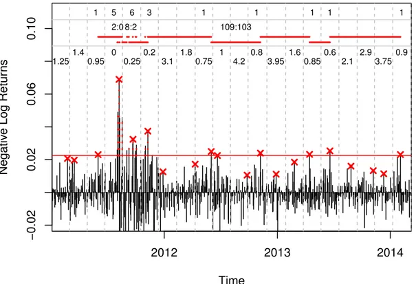
In Figure 1 we illustrate the classical blocks estimator from Section 2.4.1, the K-Gap estimator from Section 2.4.2, and the disjoint variant of the block based Maximum Likelihood estimator from Section 2.4.3 (obtained by using ˆZ_t^dj=b{1− Fˆ_n(M_t^dj)} with M_t^dj= max{ebt−1+1, . . . , e_tb} for t= 1, . . . , n/b).

The data consist of about three years of negative daily log returns on the S&P 500 index. The solid red horizontal line corresponds to the ex-post 97.5 % empirical quantile of the negative return data, i.e., u= 0.0225. Hence, we have exactly 20 values above this threshold. All exceedances of the threshold are labeled with a vertical dotted red line. The gray dashed lines mark the edges of the disjoint blocks. We choose a block length of b = 40 returns, resulting inn/b= 20 disjoint blocks.

The first line at the top of the Figure shows the empirical cluster sizes used for the disjoint classical blocks estimator from Section 2.4.1. The inverse of the average cluster size provides the classical blocks estimator for the extremal index, with a value of ˆθ^CB= 0.45 for the particular example.

The second line corresponds to the K-Gaps estimator from Section 2.4.2 with K = 6, which is depending on the threshold u and the gap parameterK, but not

2012 2013 2014

−0.020.020.060.10

Time

Negative Log Returns

1 5 6 3 1 1 1 1 1

2:0 8:2 109:103

1.25 0.95 0.25 3.1 0.75 4.2 3.95 0.85 2.1 3.75

1.4 0 0.2 1.8 1 0.8 1.6 0.6 2.9 0.9

Figure 1: This plot illustrates the three extremal index estimators described in Section 2.4. The data set consists of about 800 daily returns on the S&P 500 index from 2011-01-03 till 2014-03-10. The first line at the top documents cluster sizes, the second line shows three examples for durations and 6-Gaps, and the last line reports transformed block maxima.

the block size b. The partly displaced horizontal red lines serve as an illustration for the durations betweens exceedances. Three numerical examples are provided above those lines. For instance, 109:103 means that the inter-exceedance time was 109 days. This value, truncated with K = 6, leads to a K-Gap of 103. Since this inter-exceedance time is quite high, the truncating alters little. However, in the first example the duration is 2 results in a K-Gap of 0. The final estimated value is ˆθ^G_n = 0.51.

The blocks estimator ˆθ_n^B from Section 2.4.3 is only depending on the block size

b and is based on computing maxima within each block. In particular, such a block maximum (red crosses) can also be below the threshold, as for example for blocks 1–2 in the picture. The block maxima are then transformed to the pseudo- observations ˆZ_t^dj, which are reported in the third line of the plot. Here, the inverse of the mean yields an estimate of ˆθ_n^B= 0.62.

In this example, all estimates are quite similar and show that the negative S&P 500 returns exhibit a large degree of extremal dependence in their right tail.⁴ However, it is well know that such estimates can deviate largely depending on the estimator and parameter choice⁵.

3 Backtesting Based on the Extremal Index

If the use of correct VaR forecasts leads to an i.i.d. Bernoulli violation sequence, it seems natural to expect that there exists a VaR-adjusted return series which does not exhibit any (or only low) serial dependence, provided the true VaR^(t)_p -values are used. In fact, given some arbitrary forecasts VaRd^(t)_p , we propose to consider the following negative return-VaR ratio, defined as

e_t:=e_t(VaRd^(t)_p ) :=− r_t VaRd^(t)_p

. (3.1)

Note, the negative sign in front of the ratio, which implies that by looking at the right tail of (e_t), we essentially look at the right tail of (r_t). There is an obvious relationship with the violation sequence (It) defined in (2.1): we have {e_t>1⇔I_t = 1} and {e_t≤1⇔I_t= 0}, but (e_t) obviously contains much more information.

4This implies extremal dependence in the left tail of the S&P 500 returns.

5See for example Tables 8.1.8 and 8.1.9 in Embrechts et al. (1997).

3.1 Relative Excess Returns of Mean-Scale Models

It is instructive to first consider the relative excess return series (e_t), withVaRd^(t)_p = VaR^(t)_p , in a general mean-scale model defined by

r_t=µ_t+σ_tz_t, where z_t ^i.i.d.∼ F_z (3.2) and where E(z_t) = 0, Var(z_t) = 1 and µ_t, σ_t are Ft−1 -measurable. As a conse- quence, the conditional VaR using information up to t−1 can be written as

VaR^(t)_p =−µ_t−σ_tF_z⁻¹(p), (3.3) which implies that

et = µt+σtzt

µ_t+σ_tF_z⁻¹(p). (3.4)

We are next going to argue that the sequence (e_t) is either an i.i.d. sequence (zero mean case) or at least approximately serially independent (non-zero mean case), in particular when looking only at the left tail. This suggests to backtest the VaR- forecasts by checking for serial independence or the absence of extremal clustering of the relative excesses (e_t), as will be done in later sections.

The Zero Mean Case. Ifµ_t≡0, then Formula 3.4 simplifies toe_t=z_t/F_z⁻¹(p).

As a consequence, (e_t) is an i.i.d. sequence due to the i.i.d. property of the inno- vations (z_t).

In practice, the possibility of a non-zero mean cannot be ruled out. However, it is often argued that financial returns show only insignificant means, see, e.g., Hansen (2005). In that paper, a large number of mean-scale models is examined with respect to their volatility forecasting performance, relative to simple specifi- cations such as the classical GARCH(1,1)-model. Three different specifications for the conditional mean are used and it is concluded that the performance is almost identical across the three versions. In other words, for financial returns, the mean

is often negligible, especially in the short-term. This stylized fact is also assured by the popularity of methods and models which explicitly use the assumption of zero conditional means. A prime example is provided by the famous square-root-of-time rule for time-scaling of the volatility and VaR. The rule is well appreciated among academics and practitioners, and is even implemented in regulatory standards for VaR scaling from daily returns to 10-day-returns (see BCBS, 1996a).

The General Case. Next, consider the general case with µ_t 6= 0 being allowed.

The event{et > y}can then be rewritten as S_t(y) =

z_t < y

µ_t

σ_t +F_z⁻¹(p)

− µ_t σ_t

,

and this representation suggests that the relative excess returns are in general not serially independent: the events {e_t> y} and {e_t+1 > x} are connected through the conditional mean and volatility. However, we argue that the serial dependence is actually either vanishing or low in certain typical cases.

The first case is x= y = 1, in which case S_t(1) = {z_t < F_z⁻¹(p)} = {I_t = 1}, which is obviously independent over time. In fact, we are left with the classical violation sequence (I_t).

Next, in case of either µ_t+1 ≈ 0 or σ_t+1 → ∞, we get at least approximate equality of S_t(y) and {z_t < F_z⁻¹(p)} and hence approximate serial independence of (e_t). Note that large volatilities σ_t are typically present in periods of financial turmoil, which are in turn associated with our phenomenon of interest, that is, violation clustering.

More generally, the serial dependence vanishes forx, y ≥1 whenever−F_z⁻¹(p) µ_t/σ_tfor alltwith high probability, which is reasonable for large values ofq. In that case, S_t(y) implies z_t F_z⁻¹(p), so that only very small values of z_t may trigger the event S_t(y). Since z_t is an i.i.d. sequence, the events S_t(y) are approximately

3.2 The Backtesting Procedure for VaR

The discussion in the preceding section motivates to backtest VaR-forecasts by checking whether the relative excess sequence (et) exhibits no or only low serial dependence, especially in the right tail. As a proxy, we propose to check for extremal clustering by using the extremal index, whence the resulting test can in fact be expected to be particularly sensitive to deviations from independence in the far right tail ofet, i.e., in the most important part for risk management needs.

More precisely, recalling that an independent sequence has extremal index 1, we aim at checking for what we coin no cluster property (noc):

noc: θ_e:=θ((e_t)_t) = 1. (3.5) The backesting procedure we propose then is as follows: first, given a sequence of VaR forecasts VaRd^(t)_p and observed returns rt, for t = 1, . . . , n , calculate (et) as defined in (3.1). Second, calculate ˆθ_n = ˆθ_n(e₁, . . . , e_n) with ˆθ_n denoting any of the extremal index estimators from Section 2.4. Finally, reject the VaR-forcasts if ˆθ_n is significantly smaller than 1. Regarding the extremal index estimators, we only consider the sliding blocks estimator from Section 2.4.3 and the K-Gap estimator from Section 2.4.2; the resulting tests will subsequently be denoted by Θ^B_noc = Θ^B_noc(b) and Θ^G_noc = Θ^G_noc(u, K), respectively.

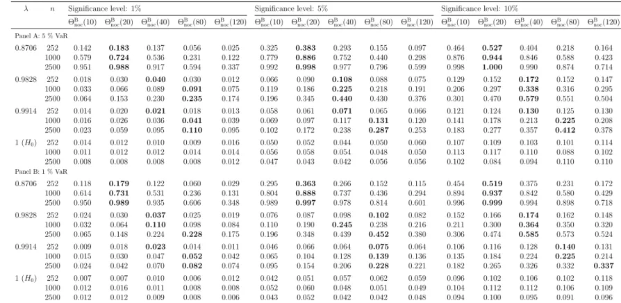
Regarding test Θ^B_noc, we first need to choose a block length parameter b. A preliminary Monte Carlo simulation study to compare several values of b; details can be found in Table 8 in Appendix A.1; guides us to choose b = 40 across all further analyses. Although more suitable choices may be possible depending on the data generating process (DGP), we set a general data-dependent strategy for the choice ofb aside, thus possibly resigning power in some cases.

Critical values for test Θ^B_noc could in principal be calculated based on the nor- mal approximation described in Section 2.4.3: if the extremal index is 1, then

θˆ_b −1 is approximately centred normal with variance 0.2726·b/n, no matter the stationary distribution Fe or the serial dependence of the time series outside the upper tail. However, the fact that the limiting distribution is pivotal also allows to approximate it by simulating from an arbitrary model for which the extremal index is 1. We hence opt for calculating critical values by first simulating ˜e₁, . . . ,e˜_n from the model

˜

e_t= r˜_t

−VaR^(t)_p , ˜r_t ^i.i.d.∼ N(0,1), VaRd^(t)_p =−Φ⁻¹(p), (3.6) where Φ denotes the c.d.f. of the standard normal distribution, and by then calculating ˆθ_n^B = ˆθ_n^B(˜e₁, . . . ,e˜_n) with the same block length parameter as chosen above, i.e.,b= 40. Note that such a simulation based approach is also common for other classical backtesting procedures where asymptotic distributions are known, e.g., for the testLR^Mar_ind defined in Section 2.2.

Let us next describe details on test Θ^G_noc, which depends on the choice of both K and u = u_n. Regarding the latter choice of u, we simply set u = 1, which essentially means that we leave the extreme value context and are back to the 0-1-violation sequence from Section 2.1 (note that e_t > 1 if and only if I_t = 1).

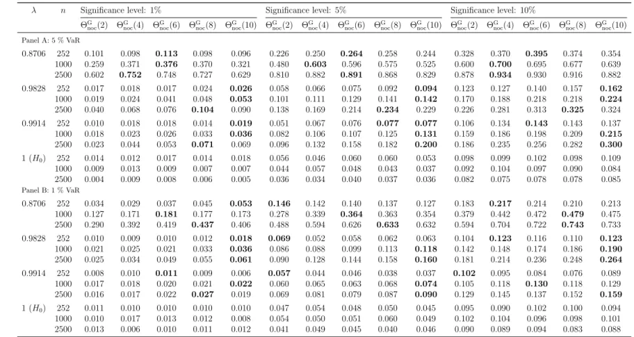
TheK-gap approach should hence rather be regarded as a classical duration-based test for the hypothesis of independence of the innovation sequence given in (2.4) (though with a different initial motivation), see also Section 2.2 for other duration- based tests.⁶ In particular, this viewpoint suggests to obtain critical values of the test simply by generating i.i.d. Bernoulli(p)-sequences ˜I_t, and to calculate θˆ_n^G= ˆθ_n^G(K) by considering each time points where ˜I_t= 1 as an exceedance (note that ˆθ^G_n only depends on those time points). Regarding the choice of the K-gap parameter, a further preliminary simulation study (details are presented in Table 7 in Appendix A.1) prompts us choose K = 6 for all further analyses.

6A more appropriate notation would hence be Θ^G_indinstead of Θ^G_noc.

Throughout this paper, the two above described simulation-based approaches, as well as all other similar approaches, are based on N = 10,000 replications, and corresponding p-values are computed as described in Appendix A.2, see also Dufour (2006).

3.3 Extensions to More General Risk Measures Including Expected Shortfall

Backtesting the Expected Shortfall (ES) recently received increased attention due to its upcoming implementation as a standard risk measure for regulatory purposes in banking (BCBS, 2016). Most available backtests of ES focus on unconditional coverage, see Kerkhof and Melenberg (2004), Wong (2008), Costanzino and Cur- ran (2015), and Kratz et al. (2018). Only recently, Du and Escanciano (2017) propose to additionally use a Box-Pierce test to test for autocorrelation in a cer- tain sequence of cumulative violations. This test can hence be regarded as the first ES backtest for independence (rather: serial uncorrelation). In this section, we extend the basic idea from Section 3.2 to obtain a further backtest for ES that is particularly sensitive to certain deviations from independence in the tails.

Recall that the main idea of the VaR method from Section 3.2 consists of checking whether the relative excess returns in (3.1) do not show any sign of ex- tremal clustering. The sensibility of such an approach was explained in Section 3.1 for mean-scale models, and the arguments can in fact be generalized to any risk measure which is translation invariant and positively homogeneous. Indeed, recall that a risk measure ρ:M →R, M a set of random variables, satisfies translation invariance if, for all R ∈ M and every c∈ R, we have ρ(R+c) =ρ(R)−c (the change of the sign stems from interpreting R as a return and not a loss). Positive homogeneity is satisfied if ρ(c R) = c ρ(R) for all R ∈ M and c > 0 (McNeil et al., 2005). By the same arguments as in Section 3.1, it is sensible to backtest a

sequence of forecasts ˆρ_t by checking whether the sequence e_t=−r_t

ˆ ρt

(3.7) does not so any sign of extremal clustering. Indeed, for location scale models as defined in (3.2) and for ˆρ_t=ρ_t=ρ(r_t| Ft−1), we obtain that

e_t =−r_t ρt

= µ_t+σ_tz_t µt−σtρ(zt),

which simplifies to Equation 3.4 if we use ρ(zt) = −F_z⁻¹(p), that is, VaR. As a consequence, it is sensible to apply the methodology described in Section 3.2 to the sequence (et)t defined in (3.7), for any translation invariant and homogeneous risk measure. We do not pursue this any further in this document.

3.4 An Extension to Distributional Backtests

The general idea from Section 3.2 may also be applied to backtesting forecasts of the entire conditional distribution (or density), see also Berkowitz (2001). More precisely, suppose that ˆFt is a distributional forecast of the conditional c.d.f. of rt

given Ft−1, the latter being denoted by F_t. The role of the VaR-adjusted return series (et) may then be played by the probability integral transform sequence

u_t = 1−Fˆ_t(r_t), t= 1, . . . , n.

In case ˆF_t=F_t, the sequence is known to constitute an i.i.d. sequence of uniformly distributed random variables on the interval [0,1], see Rosenblatt (1952). As in the previous section, a distributional backtest that is particular sensitive to deviations from independence in the upper right tail of ut is obtained by comparing the estimated extremal index of u₁, . . . , u_n with 1.

4 Size and Power Analysis

In this section, we compare our new approach to several classical backtesting procedures in terms of their empirical size and power properties. The employed alternative backtests are briefly described in Section 2.2. The results of large scale Monte Carlo simulation studies are then presented in Sections 4.1–4.5, under varying circumstances of interest.

4.1 Power Properties when True Unconditional VaRs are Used

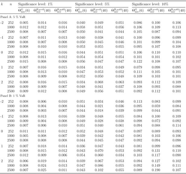
The first simulation experiment is guided by Table 4 in Ziggel et al. (2014), the purpose being to compare backtests in situations where clustered violations are likely due to the use of unconditional instead of conditional VaRs. The comparison is only carried out forindependence backtesting procedures (including the tests for noc, as the latter also have power against most deviations from ind). The data generating process is as follows:

r_t=σ_tz_t, t= 1, . . . , n, with z_t^i.i.d.∼ N(0,1), σ₁ = 1 and

σ²_t =λσ_t−1² + (1−λ)z_t−1² , t= 2, . . . , n.

As in Ziggel et al. (2014), the parameterλis chosen from the set{0.8706,0.9829,0.9914,1}

(caseλ= 1 will correspond to the null hypothesis) and the sample sizen is chosen from the set {252,1000,2500}. Note that results for sample sizes as small as 252 should be regarded with a little caution, at least for test Θ^B_noc: taking blocks of length b = 40 results in only 6 disjoint block maxima (and slightly more distinct values for the sliding block maxima), to which an exponential distribution is then

fit. However, since we do not rely on asymptotics but rather on simulation to calculate critical values, we still think that an application to such small sample sizes is sensible (and in fact, the results confirm our intuition).

Recall from Section 3.1 that the true conditional VaR of the above described model is given by VaR^(t)_p = −σ_tΦ⁻¹(p) and that the use of VaRd^(t)_p = VaR^(t)_p in formula (3.1) would result in an i.i.d. sequence of relative excess returns. Serial dependence (and in particular extremal clustering) is now introduced by instead setting VaRd^(t)_p =VaRdp (independent of t) to the empirical VaR computed from a preliminary simulation with 100,000 returns. The simulation study is performed conditional on the restriction of at least two violations per backtesting sample.⁷ As described in Section 3, the parameter b is set to b = 40 for test Θ^B_noc and to K = 6 for test Θ^K_noc.

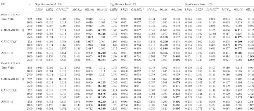
The results, namely empirical rejection rates of the competing independence backtests (calculated based on 5000 Monte Carlo repetitions), are reported in Table 1. All tests exhibit a reasonable approximation of the intended level (case λ = 1). In terms of power, the proposed extremal index tests typically yield the largest power, which on top is often much larger than for the classical competitors.

In the few cases the non-extremal index tests yield larger power, the improvement over the extremal index versions is rather small.

The rejection rates of all approaches except Θ^B_noc are decreasing in the VaR level. Clearly, the reason is that a small number of violations cannot yield the same evidence for serial dependence like a large number of violations is capable of.

For Θ^B_noc, the rejection rates change barely for varying level, a likely explanation being that the input data (relative excess returns) are approximately the same up to a scaling factor. Moreover, by construction, Θ^B_noc is also able to use information

7The probability that a generated sample of sizenviolates this condition is negligible in all cases except for the 1 % VaR level andn= 252 case, where approximately 28.2 % of randomly drawn samples exhibit at most one violation.