The Value at Risk Andreas de Vries

(1)

The Value at Risk

Andreas de Vries^∗

FH S¨udwestfalen University of Applied Sciences, Haldener Straße 182, D-58095 Hagen, Germany

May 19, 2000

1 Introduction

The main business of banks and insurance companies is risk. Banks and financial institutions lend money, running the risk of losing the lended amount, and they borrow “short money” having less risk but higher expected rates of return. Insurance companies on the other hand earn a risk premium for guaranteeing indemnifification for a negative outcome of a certain event.

The evaluation of risk is essential for both kinds of business. During the 1990’s there has been established a measure for risk in finance theory as well as in practice, theValue at Risk, VaR. It was mainly popularized by J.P. Morgan’s RiskMetrics, a database supplying the essential statistical data to calculate the VaR of derivatives.

In the context of finance Value at Risk is an estimate, with a given degree of confidence, of how much one can lose from a portfolio over a given time horizon. The portfolio can be that of a single trader, or it can be the portfolio of the whole bank. As a downside risk measure, Value at Risk concentrates on low probability events that occur in the lower tail of a distribution. In establishing a theoretical construct for VaR, Jorion [10] first defines the critical end of period portfolio value as the worst possible end-of-period portfolio value with a pre-determined confidence level “1−α”

(e.g., 99%) These worst values should not be encountered more thanαpercent of the time.

For example, a Value at Risk estimate of 1 million dollars at the 99% level of confidence implies that portfolio losses should not exceed 1 million dollars more than 1% of the time over the given holding period [10].

Currently, Value at Risk is being embraced by corporate risk managers as an important tool in the overall risk management process. Initial interest in VaR, however, stemmed from its potential applications as a regulatory tool. In the wake of several financial disasters involving the trading of derivatives products, such as the Barrings Bank collapse (see [10], regulatory agencies such as

∗e-mail: de-vries@fh-swf.de

(2)

the Securities and Exchange Commission or the BIS, in cooperation with several central banks, embraced VaR as a transparent measure of downside market risk that could be useful in reporting risks associated with portfolios of highly market sensitive assets such as derivatives. Since VaR focuses on downside risk and is usually reported in currency units, it is more intuitive than other statistical terms. It is commonly used for internal risk management purposes and is further being touted for use in risk management decision making by non-financial firms [10, 11].

However, an essential part of the balance sum of banks and financial institutions is made by the classical banking products such as credits and loans. Usually the are contracted over the counter (OTC) and are not traded on markets.

2 The concept of Value at Risk

The sample space Ω of the expected rates of return (or expected “relative returns”) r on the investment W in some arbitrary assets is mathematically represented by the set R. We assume that the expected rates of return r(t) with respect to the time horizon t of the investment is a random variable determined by the distribution functionF: Ω→[0,1],

F(x) = Z x

−∞

p(r) dr, (1)

wherepis the corresponding probability density. This means in particular that the expected rate of returnr(t) will achieve a value less thanx% (x∈R) after timetwith probabilityP r(t)5x

=

α

A A

U _| _|

| {z }

VaR/W

r p(r)

Figure 1: The Value at Risk VaR

F(x). LetΩ =e Rbe the sample space of currency-valued returns¹R=r(t)W. The expectedloss L(t) with respect to the time horizontof the investmentW then is given as thenegative difference between the return and the mean value, L(t) = µW −R(t) = (µ−r(t))W. It is a quantity in currency units (cu). Note that any return less than the expected one means an effective loss, even if it is positive. Positive values ofL(t) mean a loss after timet, negative ones a gain. Its distribution functionFe:Ωe →[0,1] is simply given byFe(L) = 1−F(L/W −µ), or

F(L) = 1e − Z L

−∞

p(L⁰/W−µ) dL⁰, (2)

with the probability density −p(L⁰/W −µ). The Value at Risk VaR with respect to the time horizon t of the investment then is defined as the maximal expected loss L(t) not exceeded with probability (1−α):

P L(t)5VaR

= 1−α, 05α51. (3)

1In this paper the following convention is valid:rdenotes a relative quantity with respect to the invested capital W of the asset (in %, say), whereasRis the absolute return in currency units (cu).

(3)

αis the default or downfall probability of the Value at Risk. For instance, according to the Basle Accord [1] it should be beα= 1%, and t = 10 days. The Value at Risk often is also called the

“unexpected loss” of the investment, cf. [12]. We haveP(L(t)5VaR) =Fe(VaR), and the Value at Risk is nothing else than the (1−α)-quantile of the random variableL(t):

VaR =Fe⁻¹(1−α), (4)

cf. [16]. To express it in terms of the expected rate of returnr(t), the Value at Risk is the negative α-quantile of the random variabler(t):

VaR = (µ−F⁻¹(α))W. (5)

Usually there only is interest on a positive Value at Risk. So we define theValue at Risk in the strict sense, VaR⁺, by

VaR⁺= max(0,VaR). (6)

In general, the Value at Risk is depending on the confidence levelα, the investment horizont, the investmentW, and the probability distribution F. According to the famous “moment problem”

the probability densityp, and thus the distributionF, is determined by the momentsmk fork= 1, 2, . . . , if and onlyF is of bounded variation on Ω, see the appendix and [20] §1.4. Thus the Value at Risk depends onmk, i.e., VaR = f·W with the functionf =fα,t(m1, m2, . . .) given as

f =µ−F⁻¹(α). (7)

As a first approximation we restrict ourselves to the first two moments,m1 andm2. But because the mean value is exactly the first moment,µ=m1, and the volatilityσis related to the second moment byσ² =m2−µ², we have approximately

VaR =fα,t(µ, σ)·W. (8)

This approximation in fact is exact for a Gaussian normally distributed random variable, for then all other moments vanish. The approximation can be generalized straightforwardly to the case of an arbitrary distribution, besides the extension to the dependence on more moments, f = f(µ, σ, m3, m4, . . .): According to the “estimating function approach” [8] one can transform the given random variable to a nearly standard distributed one.

2.1 The case of n subportfolios

Suppose a portfolio Π consisting of n subportfolios Π₁, . . . , Π_n (n ∈ N). For each subportfolio Πi we denote the rate of return by ri, or relative return, on the invested capital Wi with time horizont. In the sequel we will often callWisimply the investment of Πi. The total portfolio value is denoted by WΠ, where WΠ =Pn

i=1Wi. We suppose ri to be a real-valued square-integrable random variable with a probability distributionFi:R→[0,1].

The total volatilityσΠ of all subportfolios is given by σ_Π² = 1

W_Π²

n

X

i,j=1

ρijσiσjWiWj. (9)

Hereρ_ij are the correlation coefficients, cf. [2, 7, 15]. They form the correlation matrixCb= (ρ_ij)_i,j of r_i and r_j which has some important properties [2, 3, 7]: (i) it is symmetric, i.e.ρ_ij = ρ_ji for eachi, j= 1, . . . ,n, (ii) it is positive semi-definite, (iii) its diagonal entries are 1,ρii = 1, and (iv) its entries each have an absolute value not greater than 1,|ρij|51. The correlation matrixCb is related to the covariance matrixC= (cij) simply by the equation

C=σ^TCσ,b (10)

(4)

orcij =ρijσiσj. It is a measure of thelinear dependence ofri andrj. It induces a quadratic form Q: Rⁿ×Rⁿ→[0,∞) for two vectorsx, y∈Rⁿ by

Q(x, y) =x^TC y. (11)

The total invested portfolio capitalWΠis the sum of all individual investmentsWi of the subportfolios Πi: WΠ = Pn

i=1Wi. Accordingly, the total expected return of the portfolio Π is given by R = P

iriWi. If vi denotes the (isolated) Value at Risk of subportfolio Πi, we have vi =fiWi, according to (8). The distribution F of the total portfolio is given implicitly by the consistency condition

P

ijfifjWiWj =f²W_Π² (12)

withf =F⁻¹(α).

Let now the distributions all be Gaussian, i.e.fi =σi. Defining the vectorv= (v1, . . . , vn) we conclude that VaR² =v^TC v, orb

VaR²=P

ijρijfifjWiWj. (13)

Because VaR(λf, λ⁰W) = λλ⁰VaR(f,W), the Value at Risk VaR is a homogeneous function of degree 1 with respect to either f and W ∈ Rⁿ, if the respectively other one is held fixed.² Straightforward calculation yields

fi

∂f_i/∂σ_i

∂

∂σ_i VaR = Wi

∂

∂W_i VaR (14)

3 Models to determine the VaR

I give a short survey about most popular the basic methods to determine the Value-at-Risk, parametric models and simulations.

3.1 Parametric models

In parametric models the changes of the portfolio value obey anassumed parametric probability distribution. Under certain conditions one receives a closed analytic solution depending on the probility parameters. The simplest ones are parametric models based on the normal distribution hypothesis. Here I mention four one of these:

Portfolio-normal VaR. Here the total portfolio returnrchanges according to a normal distribution, i.e.r ∼N(µ, σ²). Then the variable transformation r 7→ z = (r−µ)/σ yieldsF as the standard normal distribution,F(x) = Φ (x−µ)/σ

. Thus for an investment the Value at Risk on the confidence level (1−α) is given by (5) as

VaR = (zασ−µ)W withzα= −Φ⁻¹(α), (15) cf. [16]. Because losses are always on one side of the distribution, for risk considerations we only regard the one-sided confidence level.

Asset-normal VaR. This is a special case of then-subportfolio case in section 2.1. The portfolio is assumed to consist ofnassetsW₁, . . . ,W_n which have normally distributed relative changesr₁, . . . ,r_n, i.e.r_i∼N(µ_i, σ_i). Then the portfolio Value-at-Risk is given by (15), with

µΠ= 1 WΠ

n

X

i=1

µiWi, σ_Π² = 1 W_Π²

n

X

i,j=1

ρijσiσjWiWj. (16)

2A rigorous mathematical introduction can be found, e.g., in [17,§26].

(5)

Both the portfolio-normal and the asset-normal distributions have little practical utility. Despite the fact that the normal distribution hypothesis is not correct, correlation estimates of a realistic n-asset portfolio has to face permanent emergence and vanishing of financial instruments, due to their individually finite maturities or portfolio extension with new positions.

Delta-normal and Delta-Gamma-normal VaR. In practice, the distributions of daily changes in many market variables have essentially fatter tails than the normal distribution. In the light of the unappropriateness of asset-normal Values at Risk it appears to be more senseful to consider m “risk factors” S(t) = (S1(t), . . . , Sn(t)) such as bond prices, interest rates, currency exchange rates, stock indices etc. The value Wi of each asset in the portfolioi then depends on these risk factors,Wi(t) =Wi(S(t)), and the corresponding expected returnRafter periodtis given by

R(t) =

n

X

i=1

W_i(t)−W_i(0).

The expected rate of returnris given byr(t) =R(t)/WΠ, withWΠ=Pn

i=1Wi(0). For example, a simple asset portfolio is a linear combination ofnstocksS, i.e.W(t) =NS(t) with then×m- matrixN with real entries. But if the assets includes options on stocks, the portfolio is not linear in the stock pricesS_i.

Fori, j= 1, . . . , m we define the parametersδ_i andγ_ij by δ_i= ∂R

∂S_i _t=0

, γ_ij = ∂²R

∂S_i∂S_j t=0

, (17)

Of course,γij=γji. By Taylor expansion we see that R(t) = X

i

δ_i∆_i(t) + 1 2

X

i,j

γ_ij∆_i(t)∆_j(t) + . . . (18) where ∆i(t) := Si(t)−Si(0). The determination of the Delta-normal VaR then starts with the approximationγij= 0 and the assumption that the ∆i’s are independent and commonly normally distributed,∆∼N(0, tC). This means that the portfolio value changeR as a whole is normally distributed, but each single position needs not to be. We then get

VaR =zα

√ t·√

d·C·d (19)

where d = (δ₁S₁(0), . . . , δ_mS_m(0)), and z_α = Φ⁻¹(α) is the α-quantile of the standard normal distribution. For details see [9, 13].

For the Delta-Gamma normal distribution the γij’s do not vanish. In this case the VaR can only be determined approximately or numerically. A broad introduction to the most commonly used methods is given in [13].

3.2 Simulation models

An alternative to parametric models are simulation models. The probability distribution of the relative returns of a portfolio emerges from a fictitious rate of return generated byscenarios.

Historical simulation or bootstrapping. The aim of this method is to generate a future distribution of possible future scenarios based on historical data. The data usually consist of daily returns forall possible assets, reaching back over a certain period. The simulation of the daily return for a day in the future then simply is done by choosing by chance (uniform distribution!) one of the historical returns.

This method is very simple to implement. Its advantages are that it naturally incorporates any correlation between assets and any non-normal distribution of asset prices. The main disadvantage is that it requires a lot of historical data that may correspond to completely different economic circumstances than those that currently apply.

(6)

Monte Carlo simulation. Monte Carlo simulation is the generation of returns (and often of asset price paths) by the use of random numbers, drawn from an assumed model distribution, to build up a distribution of future scenarios.

The VaR is calculated as the appropriate percentile of the probability distribution ofr. Suppose, for example, that we calculate 5 000 different sample values ofr. The 1-day 99% VaR is the value ofrfor the 50th worst outcome; the 1-day 95% VaR is the value for the 250th worst outcome.

The main advantages of Monte Carlo simulation are: It is the most powerful and theoretically most flexible method, because it is not restricted to a given risk term distribution; the grade of exactness can be improved by raising the sample number.

The main drawback is that it tends to be slow because a company’s complete portfolio has to be revalued many times. One way of speeding things up is to assume that equation (18) describes the relationship betweenrand theS_i’s. We then avoid the need for a complete revaluation of the portfolio. This is sometimes referred to as thepartial simulation approach.

4 How to calculate VaR

Typically the data required for the calculations of VaR are statistical parameters for the ‘underlyings’ and measures of a portfolio’s current exposure to these underlyings. The parameters include volatilities and correlations of the assets and, for longer time horizons, drift rates. In October 1994 the American bank JP Morgan introduced the systemRiskMetrics as a publicly accessible service for the estimation of VaR parameters for tradable assets such as stocks, bonds, and equities. In April 1997, JP Morgan also proposed a similar approach, together with a data service, for the estimation of risks associated with the risk of default of loans,CreditMetrics.

4.1 RiskMetrics

A detailed technical description of the method for estimating financial parameters can be found at the web sitewww.jpmorgan.com. Here I shortly describe how volatilities and correlations are estimated from historical data.

Estimating volatility. The volatility of an asset is measured as the annualized standard deviation of returns. There are many ways of taking this measurement. In RiskMetrics the volatility σion dayiis measured as the square root of a variance that is an exponantially weighted moving average (EMWA) of the square of returns,

σ²_i = 1−λ

∆t

i

X

j=−∞

λ^i−j(Rj− hRi)², (20)

where ∆tis the timestep (usually one day),Rj is the return on dayj, andhRiis the mean value over the period from dayitoj(it is usually neglected, assuming that the time horizon is sufficiently small). The parameter 0< λ51 represents the weighting attached to the past volatility versus the present return. This difference in weighting is more easily seen if we simply calculateσ_i²−λσ²_i−1 yielding (forhRi ≈0)

σ²_i =λσ_i−1² + (1−λ)Ri/∆t. (21) JP Morgan has chosen the parameter λ as either 0.94 for a horizon of one day and 0.97 for a horizon of one month.

Estimating correlation. Similarily to the estimating of volatility, RiskMetrics uses an exponantially weighted estimate

σ12,i=λσ_12,i−1(1−λ)R1,iR2,i/∆t. (22)

(7)

4.2 CreditMetrics

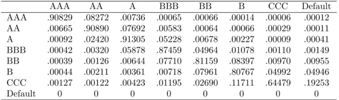
The CreditMetrics methodology is described in great detail at the web sitewww.jpmorgan.com. The corresponding dataset consists of four data kinds: transition matrices, yield curves, spread, and correlations. They depend on a model for change of credit rating: A credit rating or grade is assigned to firms as an estimate of their creditworthiness. This ususally is done by rating agencies, the famous of which areStandard & Poor’s and Moodey’s. Standard & Poor’s rate businesses as one of AAA, AA, A, BBB, BB, B, CCC, or Default. Moody’s use Aaa, Aa, A, Baa, Ba, B, Caa, Ca, C. The credit rating agencies continually gather data on individual firms and will, depending on the information, grade or regrade a company according to well-specified criteria. Migration to a higher rating will increase the value of a bond and decrease its yield, since it is less likely to default.

Transition matrices. The probability that a given company migrates to another rating class in one year’s time is given by a transition matrix M = (pij), where (pij) denotes the transition probability from rating class i to j over a given finite horizon. The matrix is time-dependent, forming aMarkov processas time passes. For instance, a typical S&P transition matrix looks like:

AAA AA A BBB BB B CCC Default

AAA .90829 .08272 .00736 .00065 .00066 .00014 .00006 .00012 AA .00665 .90890 .07692 .00583 .00064 .00066 .00029 .00011 A .00092 .02420 .91305 .05228 .00678 .00227 .00009 .00041 BBB .00042 .00320 .05878 .87459 .04964 .01078 .00110 .00149 BB .00039 .00126 .00644 .07710 .81159 .08397 .00970 .00955 B .00044 .00211 .00361 .00718 .07961 .80767 .04992 .04946 CCC .00127 .00122 .00423 .01195 .02690 .11711 .64479 .19253

Default 0 0 0 0 0 0 0 0

Unless the time horizon is very long, the largest probability is typically for the bond to remain at its initial rating.

In the CreditMetrics framework, the time horizon is one year.

Yield curves and spreads. The CreditMetrics dataset consists of the risk-freeyield to maturity for several currencies. It contains yields for maturity of 1, 2, 3, 5, 7, 10, and 30 years. Additionally, for each credit rating the dataset gives thespreadabove the riskless yield for each maturity. (Thus the spreads denote the differences between riskless bonds and a rated credit.) Evidently, the riskier

- 6

1 2 5 7 10 30 maturity

5%

10%

yield

(((

r r r r r rrisk-free

#

##

!!!

((( AA

((( ^BBB

Figure 2: Yield curve and spreads

the credit the higher the yield: Higher yield for risky credits is compensation for the possibility of not receiving future coupons or the principal. Often one also speaks of the “credit spread premium.”

(8)

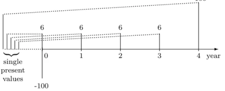
Let us examine, as a simple example, a 5-year fixed-rate loan of e100 million at 6% annual interest. The market value of the loan is equal to its present valueV,

V = 6

1 +r1+s1

+ 6

(1 +r2+s2)² + 6

(1 +r3+s3)³ + 106

(1 +r4+s4)⁴, (23) measured in millione. Herer_idenotes the risk-free rate (derived from the yield to maturity curve) expectedafter yeari, ands_i is the corresponding annual credit spread. If the loan is downgraded,

...

............

.........

........

.........

| {z } single present

values

-

-100 6

0

6

1

6

2

6

3

106

4 year

Figure 3: The cash flow and the single present values resulting from each payment.

the spreadsiwill rise, and thus the present value will fall. A credit rating upgrade has the opposite effect. Suppose that, during the first year, the borrower gets upgraded from BBB to A. ThenV is given by, say,

V = 6 + 6

1.0372+ 6

1.0432² + 6

1.0493³ + 106

1.0532⁴ =e108.66.

Hence at the end of the first year, if the loan borrower is upgraded from BBB to A, the e100 million (book value) loan has a market value ofe108.66 million.

Correlations. To examine the behavior of a portfolio of risky bonds we must consider we must consider whether there is any correlation between rerating or default of one bond to the rerating or default of another. In other words: Are bonds issued by different companies or governments correlated? The CreditMetrics dataset gives the correlations between major indices in many coun- tries.

Each company issuing bonds has the return on its stock decomposed into parts correlated with these indices and a part which is specific to the company. By relating all bond issuers to these indices we can determine correlations between the companies in our portfolio.

CreditMetrics is, above all, a way of measuring risk associated with default issues. From the CreditMetrics methodolgy one can calculate the risk, measured by standard deviation, of the risky portfolio over the required horizon. Because of the risk of default the distribution of returns is highly skewed, it is far from being normal. For details see [14,§§4 & 10], [19,§45].

Appendix: Moments and cumulants

LetX be a real random variable andpa probability distribution on the phase space Ω such that for a givenk∈Nthe expected value of|X|^k exists:

h|X|^ki= Z

Ω

|x|^kp(x) dx <∞.

Then thek-th moment, ormoment of order n, is defined by mk :=hx^ki=

Z

Ω

x^kp(x) dx. (24)

(9)

Especially the casesk= 1 andk= 2 are important: The first moment is calledmean value, µ:=

m1, and the second moment is related to thevariance σ²:=h(X−µ)²isimply byσ²=m2−µ². For details see, e.g., [4]§1.2, [5]§3, or [7]§1.

From a theoretical point of view the moments are interesting. In the famous “moment problem”

one asks: Does the knowledge of all momentsmnsuffice to determine the probability distribution?

The problem is solved by application of the fundamental Hahn-Banach theorem under quite general assumptions, eg. [20]§1.4. However, the log-normal distribution for instance has the remarkable property that the knowledge of all its moments is not sufficient to characterize the corresponding distribution, see [4]§1.3.2.

For important computational purposes it is convenient to introduce thecharacteristic function of the probability densityp(x), defined as its Fourier transformp(z):b

p(z) :=b Z

R

e^ixzp(x) dx. (25)

Sincep(x) is a probability distribution, we always havep(0) = 1. The moments ofb p(x) are easily obtained by the corresponding derivatives ofp(x) atb z= 0,

mk = (−i)^k d^k dz^k bp(z)

_z=0

. (26)

We define thek-th normalized cumulantbckof the probability distributionp(x) as thek-th derivative of the logarithm of its characteristic function:

bck := 1 (iσ)^k

d^k

dz^k logp(z)b _z=0

. (27)

We have simplybc₂ = 1. One often uses the third and fourth normalized cumulants, called the skewness bc₃and thekurtosis κ=bc₄:

bc3=

(x−µ)³ σ³

, bc4=

(x−µ)⁴ σ⁴

−3. (28)

The definitions of the cumulants may look a bit arbitrary, but these quantities have remarkable properties. For instance, they simply add by summing independent random variables. Moreover for a Gaussian distribution all cumulants of order larger than two are vanishing,bck = 0 fork=3.

Hence the cumulants, in particular the kurtosisκ, are a measure of the distance between the given probability distributionp(x) and the Gaussian distribution. For details see [4].

References

[1] Basler Ausschuss für Bankenaufsicht: Richtlinien für das Risikomanagement im Derivativgeschäft (1994);

Anderungen der Eigenkapitalvereinbarung zur Einbeziehung der Marktrisiken¨ (1996);

[2] C. Bandelow (1981):Einf¨uhrung in die Wahrscheinlichkeitstheorie.Bibliographisches Institut, Mannheim [3] H. Bauer (1991):Wahrscheinlichkeitstheorie.de Gruyter Berlin New York

[4] J.-P. Bouchaud and M. Potter (2000):Theory of Financial Risk.Cambridge University Press Cambridge [5] S. Brandt (1999):Datenanalyse.Spektrum Akademischer Verlag Heidelberg Berlin

[6] T. Br¨ocker (1995): Analysis II.Spektrum Akademischer Verlag Heidelberg Berlin Oxford

[7] M. Falk, R. Becker and F. Marohn (1995): Angewandte Statistik mit SAS. Eine Einf¨uhrung.Springer-Verlag Berlin Heidelberg

[8] V.P. Godambe (1991):Estimating Functions.Oxford University Press Oxford

(10)

[9] J.C. Hull: Options, Futures, and Other Derivatives. Second Edition.Prentice-Hall, Upper Saddle River (2000)

[10] Jorion, P. (1997): Value at Risk: The New Benchmark for Controlling Derivatives Risk, Irwin Publishing, Chicago

[11] J.P. Morgan Risk Metrics (1995): Technical Document. 4th Edition, Morgan Guaranty Trust Company, New York,http://www.riskmetrics.com/rm.html

[12] A. Lehar, F. Welt, C. Wiesmayr & J. Zechner (1998): ‘Risikoadjustierte Performancemessung in Banken’, OBA¨ 11/1998

[13] O. Read (1998): Parametrische Modelle zur Ermittlung des Value at Risk.Thesis, Wirtschafts- und Sozial- wissenschaftliche Fakultät der Universität zu Köln

[14] A. Saunders (1999): Credit Risk Measurement. New Approaches to Value at Risk and Other Paradigms.John Wiley & Inc., New York

[15] M. Steiner and C. Bruns (1994): Wertpapiermanagement.Sch¨affer-Poeschel Verlag Stuttgart

[16] M. Steiner, T. Hirschberg and C. Willinsky (1998): ‘Risikobereinigte Rentabilit¨atskennzahlen im Controlling von Kreditinstituten und ihr Zusammenhang mit der Portfoliotheorie’, in: [18]

[17] H.R. Varian (1992): Microeconomic Analysis. 3^rd Edition.Norton New York

[18] C. Weinhardt, H. Meyer zu Selhausen, M. Morlock (Eds.) (1998): Informationssysteme in der Finanzwis- senschaft.Springer-Verlag Berlin Heidelberg

[19] P. Wilmott (1998): Derivatives. The Theory and Practice of Financial Engineering.John Wiley and Sons, Chichester

[20] E. Zeidler (1995): Applied Functional Analysis. Main Principles and Their Applications.Springer-Verlag New York

References

[1] Basler Ausschuss f¨ur Bankenaufsicht: Richtlinien f¨ur das Risikomanagement im Derivativgesch¨aft (1994);