On the use of the terminal-value approach in risk-value models

https://doi.org/10.1007/s10479-020-03644-2

S . I . : R I S K M A N A G E M E N T D E C I S I O N S A N D V A L U E U N D E R U N C E R T A I N T Y

On the use of the terminal-value approach in risk-value models

Gregor Dorfleitner

© The Author(s) 2020

Abstract

We extend risk-value models for valuing streams of risky cash flows by establishing the well-known concept of terminal value in this context. For a constant growth assumption we are able to derive upper and lower bounds for the terminal value in the case of a translation- invariant and in the case of a position-invariant risk measure. For both cases we also obtain an exact formula under a special growth assumption for the future cash flows. Furthermore, we provide results on the applicability of the general findings for the case that the log-return of the risky investment follows a Brownian motion.

Keywords New approach · Business valuation · Project valuation · Terminal value · Risk measure

1 Introduction

The terminal value concept has a long-standing tradition in equity valuation (see e.g. Penman 1998; Courteau et al. 2001) and in the DCF methods used for company or project valuation (Massari et al. 2016, ch. 11). The general idea of utilizing a terminal value is that in a setting with an infinite time horizon and periodically accruing cash flows (or dividends or profits), one first assumes constant (or no) growth after a certain period. Second, the perpetuity formula is applied to find a finite present value of all those cash flows (dividends, profits) that lie after the certain period. In practical set-ups, the terminal value is used frequently (Friedl and Schwetzler 2011).

As in the traditional methods the risk of the cash flows is accounted for by the level of capital costs, i.e. as part of the discount factor, it is relatively easy to obtain terminal values of the form

C F c − g =

C F (1 + g)

(1 + c)

, (1)

B

1 Department of Finance, University of Regensburg, 93040 Regensburg, Germany

where C F represents the (annual) expected cash flow, c the cost-of-capital rate and g the (yearly) growth factor of the cash flows.

Recently, Dorfleitner and Gleißner (2018) have introduced a new valuation concept, called the risk-value-model valuation

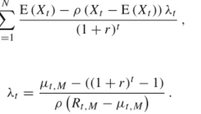
. This concept is based on certainty equivalents derived from risk measures and accounts for the risk by subtracting a (time dependent) risk premium from the expected cash flow in the numerator. In a second step, the certainty equivalent is discounted with the riskless interest rate. The concept is an appealing alternative to traditional DCF valuation methods, which are still based on the empirically falsified capital asset pricing model. However, due to the special form of the valuation formula of a single cash flow

C F

− risk ( C F

) · λ

(1 + r)

,

where λ

represents the risk premium of period t and r the riskless interest rate, the formula (1) obviously cannot be applied straight forward.

This article answers the research question under which assumptions it is possible to make use of the popular terminal value concept in the risk-value-model framework. It needs to be stated very clearly that this article is the answer to the search for suitable assumptions for upper or lower bounds or even a closed-form for the terminal value. This answer is given from a mathematical point of view. Thus, the various (and mutually exclusive) assumptions are not generally economically justified by our research, which is impossible as they are properties of the expected values and risk measures of the cash flows to be valued and their validity therefore depends on the concrete valuation problem. Thus, a potential user needs to make sure whether the required assumption for the result he or she wishes to apply can be regarded sensible for the valuation problem in which he or she wants to use the terminal value. Our research implies a large step forward for valuation practitioners, who prefer to model some periods explicitly and then make some simplifying assumptions for the rest. In this regard the model is very useful as it brings the terminal value concept into risk-value models. The (relatively new) valuation concept of risk-value models as such is useful as it enables valuation resting only upon a risk measure and the expected value, i.e. reduces informational prerequisites.

In this paper, we derive upper and lower bounds for the terminal value under a constant growth assumption. Additionally, we formulate the assumption of a special development of risk over time, which even allows us to derive an exact formula for the terminal value.

Dorfleitner and Gleißner (2018) present two ways of accounting for multi-periodicity, namely separate valuation and cumulation. We restrict ourselves to the first variant as the cumulation approach of carrying the risk to a final period appears neither to be feasible nor economically sensible for an infinite number of cash flows. The separate valuation decomposes a stream of cash flows into single cash flows, each of which is valued on a one-period basis (over a varying time interval). Those findings of Dorfleitner and Gleißner (2018) on which our considerations are based are comprehensively displayed in the“ Appendix”.

The remainder of the paper is structured as follows: In the next section, we derive general results on upper and lower bounds for the terminal value if the cash flows and their risk are expected to grow constantly. We also give an exact formula for the terminal value if the cash flows follow a special growth assumption. Sect. 3 then presents implications of the general results in the case of a Geometric Brownian motion as a model for the price dynamics of the

1While the term goes back to the work of Sarin and Weber (1993), the concept itself is different as no utility functions are needed to establish the risk-value-models valuation. Newer contributions on the topic of project selection such as Dixit and Tiwari (2020) can be seen as evidence that risk measures are indeed more and more used in project decisions.

market portfolio. In Sect. 4, we analyze the applicability of our results for the risk measures value-at-risk and standard deviation. The final section concludes with a general discussion.

2 General solutions to the terminal-value problem

To commence our considerations, let us first formulate the very problem that is to be solved.

Consider the infinite stream of cash flows X

, X

, . . . . If N is the period in which we wish to place the terminal value T V

, then the following consideration of equal present values of the original stream of cash flows and of the first N cash flows plus a terminal value implicitly defines T V

through

V

(X

) =

V

( X

) +

t=N+1

V

(X

) =

V

(X

) + T V

(1 + r)

,

where V

(.) denotes the valuation of a cash flow at time t = 0. Then we have T V

= (1 + r)

·

t=N+1

V

( X

). Note that the terminal value is not a present value, but a future value at t = N . Accordingly, throughout this paper we call N the valuation period of the terminal value and N + 1 the starting period, as X

is the first cash flow that maps into the terminal value.

As pointed out above, we next formulate different (and mutually exclusive) assumptions under which we are able to derive results for upper and lower bounds and even a for closed- form solution for the terminal value. These assumptions on the cash flows to be valued are simply stated and not economically justified here. This is because they cannot generally be justified but only in concrete application contexts, dependent on what is known about the expected value and the risk of the cash flows to be valued.

2.1 Output-oriented view with TI risk measure

Let ρ now be a TI risk measure, such as the VaR or the CVaR. In order to be able to find terminal values or at least bounds for it, it is necessary to make assumptions about the behavior of X

if t goes to infinity.

Assumption 1 (Constant growth assumption) Let E ( X

) = ( 1 + g ) E ( X

) and ρ ( X

) = ( 1 + g )ρ ( X

) for t ≥ N + 1 with − 1 < g < r.

Note that if we define X

to be equal in distribution to ( 1 + g ) X

, the constant growth assumption naturally emerges.

As all relevant risk measures are law invariant (see

“Appendix”), the constant growth assumption is uncritical from the viewpoint of the risk measure. However, in every application it needs to be clarified whether it is an acceptable model for the stream of cash flows to be valued. With this assumption a first theorem can be stated.

Theorem 1 If the risk premia (λ

)

are an increasing function in t with λ

≤ 1 for all t ≥ N + 1 and the cash flows follow the constant growth assumption from N + 1 on with ρ ( X

− E (X

)) > 0, then the terminal value at time t = N has the upper bound

2This condition is a generalization of the usual growth conditionC Ft+1= (1+g)C Ft for riskless cash flows or E

C Ft+1

=(1+g)E(C Ft)for risky cash flows whose risk is accounted for in the discount factor.

E ( X

) ( 1 − λ

) − ρ ( X

) λ

r − g (2)

and the lower bound

−ρ ( X

)

r − g . (3)

Proof To commence, we note the following two properties, which we need for our further reasoning.

( i ) E ( X

) = ( 1 + g )

E ( X

) , ρ ( X

) = ( 1 + g )

ρ ( X

) and

( ii ) E ( X

) − ρ ( X

− E ( X

)) λ

≤

≤ E (X

) − ρ ( X

− E (X

)) λ

Formally, property (i) can be proven to be a direct consequence of the constant growth assumption with complete induction, while (ii) follows from the monotonicity of (λ

)

in t and the positivity of the centered risk measure.

Now, let us consider the upper bound. We have:

T V

=

E ( X

) − ρ ( X

− E ( X

)) λ

( 1 + r )

(i)

=

t=1

(1 + g)

( E ( X

) − ρ ( X

− E ( X

)) λ

) (1 + r)

(ii)

≤

(1 + g)

(E ( X

) − ρ ( X

− E (X

)) λ

) (1 + r)

= ( E ( X

) − ρ ( X

− E ( X

)) λ

)

( 1 + g )

( 1 + r )

= E ( X

) ( 1 − λ

) − ρ ( X

) λ

r − g ,

which proves the upper bound claim. To prove the lower bound, we follow a similar reasoning:

T V

=

t=1

E (X

) − ρ ( X

− E (X

)) λ

(1 + r)

≥

E ( X

) − ρ ( X

− E ( X

))

(1 + r)

=

−ρ ( X

) (1 + r)

(i)

= −ρ ( X

)

( 1 + g )

( 1 + r )

= −ρ ( X

) r − g .

This proves the lower bound claim.

Next, we formulate an assumption under which the terminal value can be determined

exactly.

Assumption 2 (Special growth assumption I) Let E ( X

) = ( 1 + g ) E ( X

) for t ≥ N + 1 with − 1 < g < r and let the risk follow special growth according to:

ρ ( X

) = ρ ( X

) (1 + g) λ

λ

− E ( X

) (1 + g)

1 − λ

λ

for t ≥ N + 1 . (4) This assumption, which presumably hardly can be justified literally, is purely technical.

Note that the risk now scales differently to the expected value, hence there is no equality in distribution between X

and a multiple of X

anymore. Still, the assumption may serve as an approximation to reality in some cases. In any case, under this assumption a closed-form terminal value can be found.

Theorem 2 If the cash flows X

, X

, . . . follow the special growth assumption I then the terminal value at time t = N is

T V

= E ( X

) (1 − λ

) − ρ ( X

) λ

r − g (5)

Proof We start by noting some properties, which follow from the special growth assump- tion I by complete induction. As in the proof of Theorem 1, we have E ( X

) = (1 + g)

E (X

). For the risk measure, things are more complicated. We can rearrange Eq. (4) and write for t ≥ N + 1:

ρ ( X

) + E (X

) (1 + g) = ρ ( X

) (1 + g) λ

λ

+ E (X

) (1 + g) λ

λ

, which is equivalent to

ρ ( X

− E ( X

)) = ( 1 + g ) λ

λ

ρ ( X

− E ( X

)) . Therefore for an arbitrary t ≥ 1 we receive:

(∗) ρ ( X

− E (X

)) = (1 + g)

λ

λ

ρ ( X

− E ( X

)) . Now we can calculate the terminal value as:

T V

=

E ( X

) − ρ ( X

− E ( X

)) λ

( 1 + r )

(∗)

=

t=1

(1 + g)

E (X

) − (1 + g)

ρ ( X

− E ( X

)) λ

(1 + r)

= (E (X

) − ρ ( X

− E ( X

)) λ

)

(1 + g)

(1 + r)

= E ( X

) ( 1 − λ

) − ρ ( X

) λ

r − g ,

which proves the claim.

Note that the exact value under the special growth assumption equals the upper bound

under the constant growth assumption, which can be explained by a less aggressive risk

development under this assumption.

2.2 Output-oriented view with PI risk measure

Considering a PI risk measure, we begin our considerations with the constant growth assump- tion (Assumption 1 from above), in which case we can prove a slightly different theorem when compared with the case of a TI risk measure.

Theorem 3 If the risk premia (λ

)

are a decreasing function in t with λ

≥ 0 for all t ≥ N +1 and the cash flows follow the constant growth assumption from N + 1 on with ρ ( X

) > 0, then the terminal value at time t = N has the upper bound

E ( X

)

r − g . (6)

and the lower bound

E (X

) − ρ ( X

) λ

r − g (7)

Proof The terminal value can be written as T V

=

t=1

E (X

) − ρ ( X

) λ

(1 + r)

=

t=1

(1 + g)

E ( X

) − (1 + g)

ρ ( X

) λ

(1 + r)

.

From this the upper bound directly follows because we have ρ ( X

) > 0 and λ

≥ 0 for all t.

To derive the lower bound, we use the fact that (λ

)

is a decreasing function in t and thus λ

≥ λ

for all t . From this we obtain:

T V

=

(1 + g)

E (X

) − (1 + g)

ρ ( X

) λ

(1 + r)

≥

( 1 + g )

E ( X

) − ( 1 + g )

ρ ( X

) λ

( 1 + r )

= ( E ( X

) − ρ ( X

) λ

)

t=1

( 1 + g )

( 1 + r )

= E (X

) − ρ ( X

) λ

r − g .

This proves the lower bound claim.

Again, we formulate a special growth assumption in this context.

Assumption 3 (Special growth assumption II) Let the cash flows for t ≥ N + 1 fulfill E (X

) = (1 + g)E ( X

)

but the risk follows ρ ( X

) = ρ ( X

) ( 1 + g)

.

Under this, again rather technical assumption, for which the above remarks apply analo-

gously, a terminal value can be found.

Theorem 4 If the cash flows X

, X

, . . . follow the special growth assumption II, then the terminal value at time t = N is

E ( X

) − ρ ( X

) λ

r − g (8)

Proof The proof is completely analogous to that of Theorem 2, but with the utilization of the property ρ ( X

) = ( 1 + g )

ρ ( X

) , which follows directly through complete

induction from the special growth assumption II.

2.3 Input-oriented view

Practically, in the specification of Dorfleitner and Gleißner (2018), λ

exceeds every bound for t → ∞. Therefore it is sensible to assume that there is some latest period t

, after which x

= 0 so that x

=

t=1

x

. Note that the problem does not occur in the work of Dorfleitner and Gleißner (2018) as there the number of cash flows to be valued is finite.

The general valuation formula then is

t=1

E ( X

) − x

λ

(1 + r)

=

t^∗

t=1

E ( X

) − x

λ

(1 + r)

+

E (X

)

(1 + r)

. (9)

Let now E ( X

) = (1 + g) · E (X

) for t ≥ N + 1 ≥ t

+ 1 with −1 < g < r (constant growth assumption). Then a terminal can be determined in a straightforward manner.

As x

= 0 for all t ≥ N + 1, the term E ( X

) − x

λ

equals E ( X

) for t ≥ N + 1.

Then the terminal value at time t = N can be written as

T V

=

t=N+1

E ( X

)

( 1 + r )

= E ( X

)

r − g . (10)

Note that the formula is a direct application of (1) with c = r.

3 A concrete specification

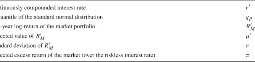
In order to specify a concrete valuation mechanism, we need to choose a model for the market portfolio return dynamics. To this end, we adhere to Dorfleitner and Gleißner (2018) and model the log-return of the market portfolio as a Brownian Motion, which implies a simple scaling of the moments along the time axis. Let μ and σ be the expected value and the standard deviation of the market portfolio’s one-year log-return R

and let r be the continuously compounded interest with r = ln(1 + r) and q

be the p-quantile of the standard normal distribution. Note that we abstain from using the subindex M for the ease of notation. Let us further assume that μ > r , which is the common assumption for the return of a risky investment. Then t μ , √

t σ and tr are the corresponding values for a t-year period.

We restrict the following analysis to the value-at-risk as TI risk measure and the standard

deviation as the PI risk measure. Although these risk measures have their limitations and

shortcomings, they still can be regarded as very popular in practice as well as in theoretical

modeling. Furthermore, a similar analysis as carried out below could of course be done for

Table 1 Overview of employed mathematical notation for the concrete specification

continuously compounded interest rate r

p-quantile of the standard normal distribution q_p

one-year log-return of the market portfolio R_M

expected value ofR_M μ

standard deviation ofR_M σ

expected excess return of the market (over the riskless interest rate) π

other risk measures such as the conditional value-at-risk. In this regard, the following is just a first step of what is possible.

Table 1 contains a brief overview of the special notation employed in this subsection.

3.1 Risk premium sequences

The formula for λ

with ρ being the (TI) value-at-risk at confidence level 1 − p (with p < 0 . 5) then is:

λ

:= e

2 2

− e

e

− e

. (11)

The proof has already been provided by Dorfleitner and Gleißner (2018).

If we specify the risk measure ρ to be the (PI) standard deviation, then λ

, according to (24), can be expressed as:

λ

:= e

2 2

− e

e

2 2

e

− 1

. (12)

The numerator is derived identically to that of (11), while the denominator emerges from the variance formula for log-normal distributions ( Johnson et al. 1994, ch. 14).

Example To illustrate the properties of the two risk premium sequences λ

t

and λ

t

, we analyze the behavior over time for a concrete very realistic parameter set, namely μ = 0 . 06, r = 0 . 02, σ = 0 . 22 and p = 0 . 5%, i.e. q

= − 2 . 576. The parameters μ and σ can be considered typical for a broad stock index (see e.g. Berk and DeMarzo 2016, ch. 10), while r = 0 . 02 represents a rather low long-run interest rate, which is however realistic for recent years. Figure 1 provides the graph of the continuous functions over time (t > 0).

3.2 General results

In order to shorten the notation in the remainder of this section, we introduce the expected excess return (over the riskless interest rate) of the market π := μ − r , which is positive according to the above assumption. Additionally, we drop the sub-index of q

and simply write q . Note that q < 0 because of p < 0 . 5.

Theorem 5 The continuous function t → λ

defined on ( 0 , ∞) starts with a value of zero

in t = 0+, then rises and has a value of one at t

=

, is larger than one beyond this

point and finally converges to 1 from above for t → ∞.

Fig. 1 Graphs of the continuous functions according toλ^{V a R}t (black line) andλt^{S D}(gray line)

Proof We commence with rewriting the risk premium λ

in the following way:

λ

= e

2 2

− e

e

− e

= 1 − e

2 2)

1 − e

(13) As all of the three terms −(π +

), q and −

are negative, both exponential terms in the numerator and the denominator vanish with t → ∞. Thus λ

→ 1.

We will use the representation (13) for the rest of this proof. From (13) we see that the value of the quotient is equal to one if and only if

−t

π + σ

2

= q √

tσ − t σ

2 ⇔ tπ = −q √

tσ .

As t > 0, this is equivalent to t =

=: t

. If t < t

, then the numerator of (13) is smaller than the numerator and thus the value of the fraction is less than one (and vice versa for t > t

).

To determine the starting point of the function at t = 0+, we need to determine the limit of the fraction according to L’Hospitale’s rule as both the numerator and the denominator are equal to zero in t = 0. Define u ( t ) = 1 − e

2

2)

and v( t ) = 1 − e

2 2

. Then (13) equals u ( t )/v( t ) . With

u (t ) =

π + σ

2

e

2 2)

and

v (t) = − qσ

2 √ t − σ

2

e

√tσ−t^σ₂²

,

we have:

t→

lim

u ( t ) v( t ) = lim

t→0+

u ( t ) v ( t ) = lim

t→0+

(π +

)e

−

−

e

= lim

t→0+

√ t (π +

)e

−

− √ t

e

= 0

−

= 0 .

Note that a mathematical treatment of the location and the uniqueness of the maximum and the exact slope behaviour of (13) on (0, ∞) is, on the one hand, not trivial and would require a lot of space. On the other hand, though, it is not really necessary as in the application the function t → λ

is only evaluated for t ∈ { 1 , 2 , . . . } . Therefore, it appears more appropriate to merely prove the rough development over time, as is done in Theorem 5, and leave a more detailed analysis, which will be required as a preparatory step when tackling a real valuation problem, to numerics. We will add more considerations in the next subsection.

Note that in any case, Theorem 1 cannot be applied in a straightforward manner because λ

is not generally smaller than 1 (nor strictly increasing in t) as after t

it takes values above 1. However, as we will see in the next subsection, Theorem 1 can still be used as a suitable approximation to the problem.

Next, we clarify the rough development over time of λ

.

Theorem 6 The continuous function according to t → λ

defined on (0, ∞) is strictly positive, it starts at a value of 0 with positively infinite slope in t = 0+, has a negative slope for every

t > t

:= − ln

2 σ²2+π σ²

2

+ π and converges to 0 for t → ∞ from above.

Proof We commence with rewriting the risk premium (12) in the following way:

λ

= e

2 2

− e

e

2 2

e

− 1

= 1 − e

2 2)

e

− 1 . (14)

Now, obviously, e

2

2)

is less that one for t > 0 and converges to 0 for t → ∞, while e

− 1 > 0. Thus, (14) has a positive value. Concerning the limit behavior, we observe that for t → ∞ the numerator converges to 1, while the denominator exceeds every bound.

Therefore, λ

→ 0.

To determine the starting point of the function at t = 0+, we need to determine the limit of the fraction according to L’Hospitale’s rule as both the numerator and the denominator are equal to zero in t = 0. We define u ( t ) = 1 − e

2

2)

and v( t ) =

e

− 1. Then (14) equals u ( t )/v( t ) . With u ( t ) = (π +

) e

2

2)

and v ( t ) =

2

√

e^tσ2−1

, we have:

t→0+

lim u(t) v(t) = lim

t→0+

u (t) v (t) = lim

t→0+

(π +

)e

e^tσ2σ₂²

√

e^tσ2−1

= lim

t→0+

2 (π +

) e

e

− 1

σ

= 0

σ

= 0

To investigate the slope claims, we consider the first derivative according to the quotient rule. First we calculate u ( t )v( t ) − u ( t )v ( t ) as

π + σ

2

e

2 2)

e

− 1 −

1 − e

2

2)

e

e

− 1 . (15) Next, we multiply (15) with

e

− 1, which corresponds to expanding the first derivative of u ( t )/v( t ) with this term. This yields:

π + σ

2

e

2

2)

e

− 1 −

1 − e

2 2)

e

σ

2 =

= π + σ

e

2 2)

−

π + σ

2

e

2 2)

− σ

2 e

(16)

To determine the limit of the first derivative at t = 0 + , we observe that the numerator (16) and the denominator e

− 1

both vanish at zero and therefore apply L’Hospital’s rule. We have

t→0+

lim d dt

u(t ) v(t) = lim

t→0+

π + σ

e

2

2)

− (π +

)e

−

e

e

− 1

= lim

t→0+

−

π + σ

π −

e

2

2)

+ (π +

)(π +

)e

−

e

3

e

− 1e

= lim

t→0+

π 1 +

3

e

− 1 = +∞ . (17)

Now let us assume that t > t

. This is equivalent to

−t

π+σ² 2

<ln σ²

2

σ²+π ⇔ e^−t(π+σ

2 2)< ^σ

2

2

σ²+π ⇔ π+σ²

e^−t(π+σ

2 2 )< σ²

2 .

With this, (16) can be written ase

π + σ

e

2 2)

−

− π +

e

2 2 )

, which is obviously less than zero. Therefore, the sign of the derivative of t → λ

is negative

for all t above the positive figure t

.

Note that after starting with a positive slope, the function necessarily possesses a local maximum somewhere between 0 and t

. Again, we abstain from searching the exact locations of the maxima as this has to be done numerically as a preparatory step of the valuation procedure.

3.3 Application, numerical examples and results

Let us now apply the general results for the specific interpretations of λ

introduced in

this section. We start with the TI risk measure, i.e. the VaR, and a cash flow X

with

E ( X

) = 2 and ρ ( X

) = − 1. Note that the latter implies ρ ( X

− E ( X

)) = 1 and therefore still guarantees a value reduction due to risk. Let us further assume that the growth factor is g = 0 . 01.

Theorem 1 Now reverting to Theorem 1, we have to state that the behavior of λ

over time is such that the assumptions of the theorem are not valid. However, knowing that λ

converges to 1, the result on the upper bound can be used from a certain N

onwards. The result on the lower bound is, strictly speaking, not applicable. However, in reality, for many parameter values the maximum value above 1 is so extremely close to 1 that it still makes no difference numerically.

Example Let us continue the example from above with π = 0.04, r = 0.0202, σ = 0.22 and p = 0.5%, i.e. q

= −2.576. For these values, the function λ

strictly increases on t ∈ {1, 2, . . . , 220} and reaches its maximum at 220 with a value of 1.000000356, which is a relative error of less that one millionth and therefore surely negligible.

Thus we have an (approximate) lower bound of

−ρ ( X

)

0.0202 − 0.01 = 1

0.0102 = 98.03 .

The upper bound according to Theorem 1 for the starting period N + 1 = 11 is 2 ( 1 − λ

) − 1 · λ

0.0202 − 0.01 = 139.83,

while for N = 20 (50) it takes a value of 120.08 (101.25). A rough approximation of the real terminal value could then be to take the arithmetic mean of both bounds yielding the estimates 118.93 (N = 10), 109.05 (N = 20) and 99.64 (N = 50). The real terminal values, according to deeper numerical analysis

, are 103.88 (N = 10), 101.11 (N = 20) and 98.47 (N = 50). While in the latter case the approximate value is already relatively close, the upper bound is generally not as close to the real value as the lower bound.

Theorem 2 Theorem 2 can of course simply be applied and yields the value of the upper bound of the above example. The question of interest is, which implications follow for the modelling of the cash flows and whether these are realistic. Starting in t = N + 1, the model for the risk of the future cash flows is

ρ ( X

) = 1.01

· λ

λ

(ρ ( X

) + E ( X

))

−1.01

· E ( X

) = 1.01

· λ

λ

· 1 − 2

.

Figure 2 illustrates the development of the risk over time under the special growth assumption for different starting periods. It surely will be hard to find application cases in which the risk of the cash flows exactly evolves like that. However, it is not completely impossible and may be justifiable as an approximation to reality in some settings, especially for late starting periods (cf. the gray solid line).

Next, we consider the standard deviation as risk measure and Theorem 3 and Theorem 4.

Here, we again assume g = 0.01, E ( X

) = 2, but now ρ ( X

) = 1.

3This analysis is based on the numerical calculation of the sum(1+r)^N·_L

t=N+1V₀(Xt)for a value of Lthat is so high that increasingLat most changes the numerical value by less than 10⁻⁷. Here, a value of L=3000 is sufficient and, thus, practically the proxy for infinity.

Fig. 2 Graphs of the VaR development according to the special growth assumption dependent on the number of periods after valuation periodNforN=10 (gray dotted line),N=20 (black dotted line) andN=50 (gray solid line). For comparison, the black solid line displays the exponential growth development withg=0.01, i.e. the constant growth assumption

Theorem 3 We can state that the behavior of λ

over time is such that the assumptions of Theorem 3 are fulfilled, at least in any case in which the starting period of the terminal value N + 1 lies right of t

.

Example Let us continue the example from above with the same parameter values. For these values the function λ

strictly increases on t ∈ {1, 2, . . . , 12} and reaches its maximum at 12 with a value of 0.6053. After this instant of time, λ

decreases against 0. From the fact that t

is 22.18, we can derive the information that t ≥ 23 is a sufficient but not necessary condition for a decreasing λ

function. The upper bound according to Theorem 3 is

= 196.05 .

The lower bound for N + 1 = 12 is

E ( X

) − ρ ( X

) λ

0.0202 = 136.71 .

while for N = 20 and N = 50 it takes the values 140.58 and 166.66, respectively. A rough approximation of the real terminal value could then be to take the arithmetic mean of both bounds yielding the estimates 166.38 (N = 12), 168.32 (N = 20) and 181.36 (N = 50).

The real terminal values are 175.66 (N = 12), 178.78 (N = 20) and 187.54 (N = 50). In these cases, the rough estimates are relatively close to the real values.

Theorem 4 Again, the Theorem 4 can be applied without any problems and yields the lower bound of the above example. However, the special growth assumption II implies a risk struc- ture over time as follows. Starting at t = N + 1, the model for the risk of the futures cash flows must follow

ρ ( X

) = 1 . 01

· λ

λ

ρ ( X

) = 1 . 01

· λ

λ

.

Dependent on the starting period of the terminal value N + 1, this can have severe conse-

quences. Figure 3 depicts the development of the risk over time implied by the special growth

Fig. 3 Graphs of the standard deviation development according to the special growth assumption II dependent on number of periods after valuation periodN forN =5 (gray dotted line),N =12 (black dotted line), N=20 (gray solid line) andN=50 (black solid line)

assumption II for several starting periods. Note that risk increases over time much faster than with growth rate g = 0 . 01.

Thus, such a risk development may be regarded realistic only in rare cases. Additionally, a risk evolution as displayed by the gray dotted line (first decreasing, then increasing risk) appears to be extremely specific.

4 Further numerical results and practical considerations

In order to abstract from the concrete example, we conduct a more detailed analysis on the location of the maxima of both risk premium sequences. It is necessary to know about these maxima to be able to apply Theorem 1 and Theorem 3, which build on monotonicity beyond a certain instant of time. We present the results of a systematic numerical investigation in Tables 2 and 3. To this end, we vary the market risk premium π from 0.02 to 0.06 and the volatility of the market from at least 0.14 to at most 0.30 to represent the range of realistic values that could result from statistical estimations or future scenario analysis. In the case of λ

, we also vary p from 0.1% to 1%. Note that in the case of a real valuation problem, we also need to specify the interest rate r. However, for a calculation of the lambdas, the mentioned parameter settings are sufficient. Building on the general curve sketching results of Theorem 5 and 6, we only need to calculate the values of λ

for discrete instants of time t = 1, 2, . . . and stop as soon as the slope changes.

The most important findings of this analysis are as follows. In Table 2 one can observe the fact that the deviation from 1 at the maximum of t → λ

is rather negligible. Only in some rather implausible combinations of high market risk premia and low volatility is the deviation larger than 1% (marked by bold digits). The worst case is the parameter setting of π = 0 . 06, σ = 0.14, p = 0.01 with a deviation of approximately 3.26%. Altogether, the maximum

4Indeed, 1.01⁵⁰=1.64, while even forN=5 we have a factor of more than three after 50 periods.

Table 2 Discrete instants of time whereλ^{V a R}t is maximal dependent on a broad variety of realistic values of σandπ.

σ π

0.02 0.025 0.03 0.035 0.04 0.045 0.05 0.055 0.06

Panel A:p=0.001

0.14 510 337 241 183 145 118 99 84 73

0.16 648 424 301 227 178 144 120 101 87

0.18 805 525 371 277 216 174 144 121 104

0.2 909 637 449 334 260 208 171 144 123

0.22 847 761 535 398 308 246 202 169 144

0.24 767 696 618 467 361 288 236 197 167

0.26 696 637 587 545 418 334 273 227 192

0.28 633 584 541 505 473 381 313 260 220

0.3 576 535 500 468 441 404 354 296 250

Panel B:p=0.005

0.14 368 246 178 137 110 90 76 66 57

0.16 462 305 219 166 132 108 90 77 67

0.18 570 374 266 201 158 128 106 90 78

0.2 693 451 319 239 187 151 125 105 91

0.22 811 538 379 283 220 177 146 122 105

0.24 767 625 445 331 256 205 169 141 121

0.26 696 637 511 383 296 237 194 162 138

0.28 633 584 526 438 340 271 222 185 157

0.3 576 535 500 455 383 308 251 209 177

Panel C:p=0.01

0.14 308 208 152 118 95 79 67 58 51

0.16 384 255 184 141 112 93 78 67 58

0.18 471 310 222 168 133 109 91 77 67

0.2 570 373 265 200 157 127 105 89 77

0.22 681 443 313 234 183 148 122 103 88

0.24 735 520 366 273 213 171 141 118 101

0.26 696 589 424 316 245 196 161 135 115

0.28 633 584 479 362 280 224 183 153 130

0.3 576 535 485 410 318 254 207 173 147

The figures in bold digits represent those cases where the maximum value deviates more than 1% from the value of 1. In all other cases the deviation is less than 1%

lambda value is reached relatively late, so that the assumption of strictly increasing λ

can be maintained as an approximation to reality for every starting period. Note that the above example can be found in Panel B in the middle of the table.

The case of λ

is presented in Table 3. Here we can observe relatively low values of

maximizing t. Thus Theorem 3 can be applied for starting periods in the range of around 10 to

20. Also, Theorem 4 can be applied with relatively early starting periods without exhibiting

the—possibly implausible—behavior of first decreasing and then increasing risk (cf. red line

Table 3 Discrete instants of time whereλt^{S D}is maximal dependent on a broad variety of realistic values ofσ andπ

σ π

0.02 0.025 0.03 0.035 0.04 0.045 0.05 0.055 0.06

0.14 27 25 22 21 19 18 17 16 15

0.16 23 21 20 18 17 16 15 14 13

0.18 20 19 17 16 15 14 14 13 12

0.2 17 16 15 14 14 13 12 12 11

0.22 15 14 13 13 12 12 11 11 10

0.24 13 13 12 11 11 10 10 10 9

0.26 12 11 11 10 10 9 9 9 8

0.28 10 10 9 9 9 9 8 8 8

0.3 9 9 9 8 8 8 7 7 7

in Fig. 3). Such behavior only occurs if the starting period lies before the maximizing t of Table 3.

5 Discussion and conclusion

In this paper, we extend risk-value models for valuing streams of risky cash flows by intro- ducing the concept of terminal value to this framework. As the case of the input-oriented perspective is treatable in a simple manner, the main focus is on the output-oriented view.

For a constant growth assumption, upper and lower bounds for the terminal value in the case of a translation-invariant and in the case of a position-invariant risk measure can be derived. For both cases, we also derive an exact formula, however only under a special growth assumption for the future cash flows, which can be characterized as unrealistic for many application cases, especially in case of the standard deviation being the risk measure.

However, the aim of this article is not to provide an economic justification for the assumptions but rather to clarify which assumptions are required to be able to use terminal values or at least upper and lower bounds for these. Furthermore, we demonstrate how the general findings can be applied under the assumption that the price of the market portfolio follows a Geometric Brownian motion. It becomes apparent that in the value-at-risk case under this assumption the prerequisites of the lower bound result are not fulfilled literally. However, for realistic parameter values the corresponding theorem can still serve as an approximation.

As a concrete consequence for applying Theorems 1 to 4, it appears to be advisable to apply these for rather late starting periods N + 1, in which case the arithmetic mean of the upper and the lower bound appears to be a relatively good approximation of the correct value.

If the cash flow modeling requires relatively early terminal values (say: at N = 5), then one can simply valuate the first periods after the staring period separately (say: from 6 to 30) and only use the terminal value formulae afterwards (say: for N = 30). Generally, the upper and lower bound results may be more beneficial for realistic cash flow modeling situations than the closed-form exact terminal value due to the corresponding required assumptions.

Summarizing, the concept of terminal value can in principal be used in risk value models,

but only with certain caveats and limitations. This paper therefore marks a significant progress

compared with the original framework of Dorfleitner and Gleißner (2018), in which a final

cash flow at some period is required. Generally, it should be noted that as in usual DCF models the value of the stream of cash flows is very sensitive to the specification of the growth rate (Friedl and Schwetzler 2011).

Several generalizations of the concept could be investigated in the future. One idea is to overcome the Brownian motion hypothesis to calculate explicit risk premium sequences.

Other dynamics such as dynamics with jumps or long-time mean-reverting processes for the stock price process are also conceivable. Moreover, as with this research risk-value models are also established over an infinite time horizon, it may be an interesting task to investigate whether dynamic (i.e. multi-period) risk measures as introduced by Riedel (2004) can be utilized for a generalisation of the imperfect replication approach. However, it is unclear at the moment how the initial approach of Dorfleitner and Gleißner (2018) is to be generalized that this becomes possible.

In any case, the results found in this paper can be very useful for practitioners, who prefer to model some periods explicitly and then make some simplifying assumptions for the rest.

In this regard our contribution extends this concept to risk-value models or at least shows under which assumptions it can be used.

Acknowledgements Open Access funding provided by Projekt DEAL.

Open Access This article is licensed under a Creative Commons Attribution 4.0 International License, which permits use, sharing, adaptation, distribution and reproduction in any medium or format, as long as you give appropriate credit to the original author(s) and the source, provide a link to the Creative Commons licence, and indicate if changes were made. The images or other third party material in this article are included in the article’s Creative Commons licence, unless indicated otherwise in a credit line to the material. If material is not included in the article’s Creative Commons licence and your intended use is not permitted by statutory regulation or exceeds the permitted use, you will need to obtain permission directly from the copyright holder.

To view a copy of this licence, visithttp://creativecommons.org/licenses/by/4.0/.

Appendix A: A short recapitulation of risk-value-model valuation A.1 Basics

Risk-value model valuation according to Dorfleitner and Gleißner (2018) essentially builds upon a risk measure to determine and quantify the notion of risk and scales the reference investment in a way that it has the same risk as the cash flow to be valued. Thus, we shortly state some necessary essentials about risk measures, which can generally have several properties.

For risk-value models three properties are of importance. Let

be the set of all real-valued random variables on the probability space (, ,

) with existing finite values of ρ ( X ) for X ∈

. Then we define:

• positive homogeneity (PH) through ρ(c X ) = cρ(X) for all c ≥ 0, X ∈

,

• translation invariance (TI) through ρ( X + c ) = ρ( X ) − c for all c ∈ IR, X ∈

and

• position invariance (PI) through ρ( X + c ) = ρ( X ) for all c ∈ IR, X ∈

.

The prerequisite for risk-value model valuation is the use of a PH risk measure that is

simultaneously either TI or PI. Therefore, the expected shortfall, also called conditional

value-at-risk, (see e.g. Acerbi and Tasche 2002; Inui and Kijima 2005; Bamberg and Neuhierl

2010) and the value-at-risk are suited as they both are PH and TI. Moreover, PH risk measures

fulfilling the PI property such as the standard deviation or TI-variants of PI risk measures,

i.e. risk measures applied to X − E ( X), which are also deviation measures (Righi 2019), can

serve as basis of risk-value-model valuation.