Stellar Motion Near the Supermassive Black Hole in the Galactic Center

Stellar Motion

Near the Supermassive Black Hole in the Galactic Center

INAUGURAL-DISSERTATION

zur

Erlangung des Doktorgrades

der Mathematisch-Naturwissenschaftlichen Fakultät der Universität zu Köln

vorgelegt von

Marzieh Parsa aus Shiraz, Iran

Köln 2018

Berichterstatter: Prof. Dr. Andreas Eckart

Prof. Dr. J. Anton Zensus

Tag der mündlichen Prüfung: 10. Oktober 2017

Abstract

General relativity is the least tested theory of physics. The close environment of the supermassive black hole provides us with the perfect laboratory for the investigation of the predictions of this theory. Therefore, the Observation of S-stars in the Galactic center in the near-infrared wavelengths provides the opportunity to study the physics in the vicinity of a supermassive black hole and conduct unique dynamical tests of the theory of general relativity.

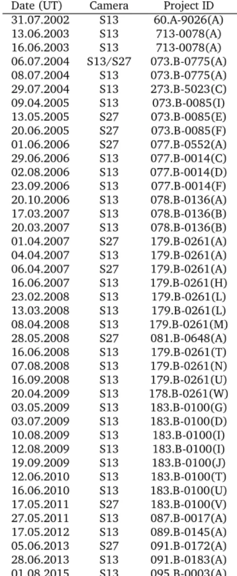
In my thesis, I use near-infrared high angular resolution adaptive optics images of the central stellar cluster acquired with the NACO instrument at the Very Large Telescope of the European Southern Observatory, from 2002 to 2015. In addition, I employ the published astrometric and line of sight velocity data obtained with the Keck telescope from 1995 to 2013.

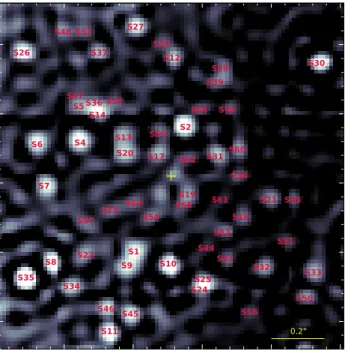
I use the SiO maser sources in the wide field of view of the NACO S27 camera.

The positions and motions of these maser sources and the position of Sgr A*, the supermassive black hole in the center of the Galaxy, is known in the radio regime. Therefore, I find the connection between the near-infrared data and the radio reference frame. Next, I connect the images of the S27 camera to the images of the S13 camera, in which the S-stars are observable in the central arcsecond, using six overlap stars. Moreover, I use the linear motion of five isolated S-stars to overcome the small distortion in the images of NACO. Then I focus on the three stars known to have the shortest orbital periods, i.e., S2, S38, and S0-102 (also known as S55). I extract the astrometric positions of these three stars in the near- infrared reference frame. Using the astrometric and radial velocity data, I calculate their six Keplerian orbital elements and the gravitational potential parameters of Sgr A*, simultaneously. To calculate the orbits, I apply the fourth-order Runge- Kutta integration technique on equations of motion with both the Newtonian and first-order post-Newtonian relativistic models. I use a minimum χ

method for the fitting procedure and evaluate the uncertainties by the Markov Chain Monte Carlo technique. The important results from the procedure are an estimate of the central mass of M

= (4.15 ± 0.13 ± 0.57) × 10

M and the distance to the Galactic center of R

= 8.19 ± 0.11 ± 0.34 kpc.

In addition, since S2 is on an orbit with a short orbital period and a large eccentricity, it motivates me to develop a practical method to probe the general relativistic effects introduced by the strong gravitational potential of the supermas- sive black hole. I find a correlation between the deviation of a relativistic orbit from a Keplerian one and a suitable relativistic parameter. I choose the relativistic parameter Υ ≡ r

/r

, with r

being the Schwarzschild radius of the black hole and r

the impact parameter, i.e., the closest approach. The deviation of a first-order post-Newtonian orbit from a Keplerian one can be seen as the changes of orbital

i

ii ABSTRACT

parameters, such as the semimajor axis, eccentricity, and the argument of periapse.

The semimajor axis and eccentricity change when comparing the upper and lower halves of the orbit, and the argument of periapse changes when comparing the pre- and post-periapse halves of the orbit. To find the correlation, I use a first-order post-Newtonian approximation to simulate the orbits of several stars with a wide range of periapse distances lying inside the orbit of S2. The found correlation is then applied on S2.

For the orbit of S2, with the mass of the black hole and the orbital parameters calculated previously, I expect a relativistic parameter of Υ = 0.00065 from theory.

Using this new method, I find a value of Υ = 0.00088 ± 0.00080, which is within the uncertainty in agreement with the expected theoretical value. Moreover, for the variations in the argument of periapse of S2, I find ∆ω = 14

± 7

, which agrees with the theoretical periapse shift of 11

. Finally, I rule out any other perturbing effect that could generate the similar results, such as the noise on the stellar positions, rotation of the image, or the drifts of the black hole. My analysis shows for the first time that the subtle effects predicted by general relativity on the orbits of stars close to the supermassive black hole, can be obtained from our current observations.

S2 is the first star on an orbit around a supermassive black hole for which a

post-Newtonian effect has been measured.

Zusammenfassung

Die Allgemeine Relativitätstheorie ist die am wenigsten getestete Theorie der Physik.

Die nächste Umgebung eines supermassiven schwarzen Lochs bietet den perfekten Ort um die Vorhersagen der Allgemeinen Relativitätstheorie auf die Probe zu stellen.

Daher eröffnet die Beobachtung der im Zentrum der Milchstraße befindlichen S- Sterne, im nahen infraroten Wellenlängenbereich, die Möglichkeit die Physik in der nächsten Umgebung eines supermassiven schwarzen Lochs zu erforschen und somit einzigartige Tests der Allgemeinen Relativitätstheorie durchzuführen.

In meiner Dissertation verwende ich durch die adaptive Optik hoch aufgelöste Bilder des zentralen Sternenclusters, aufgenommen im Zeitraum von 2002 bis 2015 im nahen Infrarot mit dem Instrument NACO der Europäischen Südsternwarte am Very Large Telescope. Zusätzlich verwende ich veröffentlichte astrometrische und Radialgeschwindigkeitsdaten, die mit dem Keck Teleskop im Zeitraum von 1995 bis 2003 aufgenommen wurden.

Ich konzentriere mich auf die drei Sterne mit den kürzesten bekannten Um- laufperioden, d.h., S2, S38 und S0-102 (auch bekannt als S55). Ich extrahiere die astrometrischen Positionen dieser drei Sterne im nahen infraroten Referenz- bild. Ich verwende die SiO Maser-Quellen, die sich im großen Gesichtsfeld der NACO S27 Kamera befinden. Die Positionen und Bewegungen dieser Maser-Quellen und die Position von Sgr A*, dem supermassiven schwarzen Loch im Zentrum der Galaxie, sind im Radiobereich bekannt. Auf diese Weise finde ich eine Ver- knüpfung zwischen den Daten im nahen Infrarot und dem Radio Referenzbild.

Danach verknüpfe ich die Bilder der Kamera S27 mit denen der Kamera S13, auf welcher die S-Sterne in der zentralen Bogensekunde beobachtbar sind, in- dem ich sechs Sterne übereinander positioniere. Des Weiteren verwende ich die Linearbewegung von fünf isolierten S-Sternen um für die geringe Verzerrung der NACO-Bilder korrigieren zu können. Unter Verwendung der astrometrischen und Radialgeschwindigkeitsdaten von S2, S38 und S0-102 bestimme ich gleichzeitig deren sechs Kepler-Umlaufbahn-Elemente und die Parameter zur Beschreibung des Gravitationspotentials des supermassiven schwarzen Lochs Sgr A*, in welchem sich der S-Sternhaufen befindet. Zur Berechnung der Umflaufbahnen wende ich die Runge-Kutta Integrationstechnik vierter Ordnung auf die Bewegungsgleichung an, sowohl mit Newtonschen als auch post-Newtonschen relativistischen Modellen erster Ordnung. Die Fitprozedur wird mit der Minimum-χ

-Methode durchgeführt und die Ungenauigkeiten werden mit Hilfe der Markov Chain Monte Carlo Tech- nik bestimmt. Die wichtigen Ergebnisse dieser Prozedur sind die Abschätzung der zentralen Masse M

= (4.15 ± 0.13 ± 0.57) × 10

M und die Entfernung zum Galaktischen Zentrum R

= 8.19 ± 0.11 ± 0.34 kpc.

Die Tatsache, dass S2 sich auf einer Umlaufbahn mit kurzer Umlaufperiode und

iii

iv ZUSAMMENFASSUNG

hoher Exzentrizität befindet, motiviert mich dazu eine neuartige und praktische Methode zum Erproben der Effekte der Allgemeinen Relativitätstheorie starker Gravitationspotentiale zu entwickeln. Mein Ziel ist es, eine Korrelation zwischen der Abweichung der relativistischen Umlaufbahnen zu den Kepler-Umlaufbahnen und einem relativistischen Parameter zu finden. Hierzu wähle ich den relativistischen Parameter Υ ≡ r

/r

, wobei r

der Schwarzschildradius des schwarzen Lochs und r

der Stoßparameter ist. Die Abweichung einer post-Newtonschen Umlaufbahn erster Ordnung von einer Keplerschen Umlaufbahn kann als Änderung der Umlauf- bahnparamter, wie der großen Halbachse, der Exzentrizität und des Arguments der Periapsis angesehen werden. Die große Halbachse und die Exzentrizität än- dern sich bei Vergleich der oberen und unteren Hälfte der Umlaufbahn, und das Argument der Periapsis ändert sich, wenn die vor- und nach-Periapsis Hälften der Umlaufbahn verglichen werden. Zur Bestimmung der Korrelation verwende ich eine post-Newtonsche Näherung erster Ordnung um die Umlaufbahnen mehrerer Sterne, mit einer weiten Auswahl an Periapsisabständen, die sich alle innerhalb der Umlaufbahn des Sterns S2 befinden, zu simulieren. Die gefundene Korrelation wird dann auf S2 angewandt.

Für die Umlaufbahn von S2 erwarte ich einen relativistischen Parameter Υ =

0.00065 aus der Theorie, unter der Verwendung der zuvor bestimmten Masse des

schwarzen Lochs und der Umlaufbahnparameter. Ich erhalte einen Wert des relati-

vistischen Parameters von Υ = 0.00088 ± 0.00080, welcher innerhalb des Fehlers

mit dem erwarteten theoretischen Wert übereinstimmt. Des Weiteren erhalte ich für

die Änderung des Arguments der Perisapsis der Umlaufbahn von S2 einen Median

mit einer absoluten Medianabweichung von ∆ω = 14

± 7

, welcher konsistent mit

der theoretischen Periapsisänderung von 11

ist. Daraufhin schließe ich Störeffekte

aus, die ähnliche Resultate erzeugen können, wie Abweichungen in den Positionen

der Sterne und in der Rotation des Bildfeldes oder der Verschiebung des schwarzen

Lochs. Meine Untersuchung zeigt zum ersten mal, dass die feinen Effekte, die von

der Allgemeinen Relativitätstheorie für Sterne, die sich auf engen Umlaufbahnen

um das schwarze Loch befinden, aus unseren Beobachtungen bestimmt werden

können. S2 ist der erste Stern auf einer Umlaufbahn um das supermassive schwarze

Loch, für den ein post-Newtonscher Effekt gemessen wurde.

Contents

Abstract i

Zusammenfassung iii

Contents v

1 Introduction 1

1.1 The Galactic Center . . . . 1

1.1.1 The Supermassive Black Hole in the Galactic Center . . . . . 1

1.1.2 The Dynamical Components of the Galactic Center . . . . . 3

1.1.3 The S-cluster . . . . 6

1.2 Keplerian Orbits . . . . 10

1.3 General Relativity and Black Holes . . . . 12

1.3.1 Post-Newtonian Approximation . . . . 13

1.3.2 Relativistic Interactions with a Supermassive Black Hole . . 14

1.4 Observation and Data Reduction . . . . 16

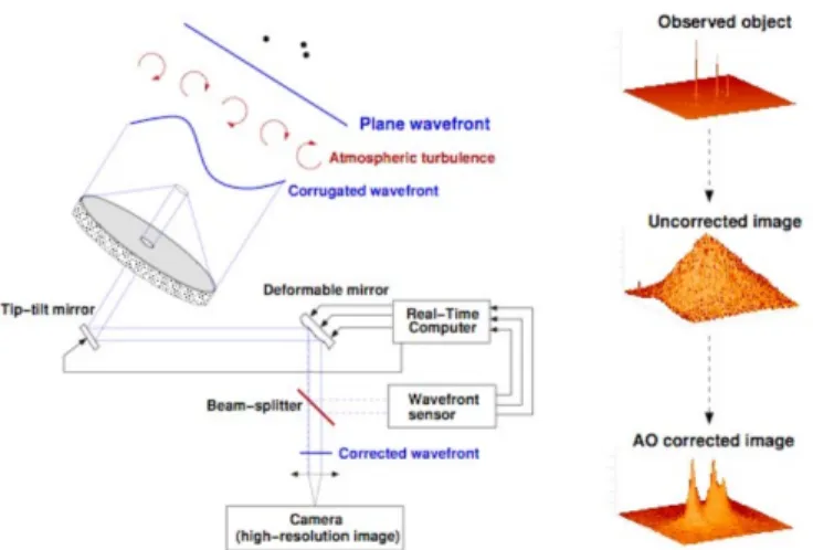
1.4.1 Observations . . . . 16

1.4.2 Adaptive Optics . . . . 17

1.4.3 Data Reduction . . . . 18

1.4.4 Deconvolution . . . . 19

1.5 Dissertation Outline . . . . 20

2 Stellar Positions and Orbits in the Galactic Center 23 2.1 Introduction . . . . 23

2.2 Observations . . . . 24

2.3 Near-Infrared Data . . . . 24

2.3.1 Astrometric Accuracy . . . . 27

2.3.2 Connection between the NIR and Radio Reference Frames . 27 2.3.3 Derivation of the Positions . . . . 30

2.4 Newtonian and Relativistic Models . . . . 37

2.5 Stellar Orbits . . . 41

2.6 Discussion . . . . 43

2.6.1 Comparison to the Litrature . . . . 43

2.6.2 Overcoming the Bias in the Orbital Fitting . . . . 44

3 Relativistic Orbit of the Stars Near the Black Hole in the Galactic Center 47 3.1 Introduction . . . . 47

3.2 Near-Infrared Data . . . . 48

v

vi CONTENTS

3.3 The Case of Simulated Stars . . . . 48

3.4 Method for the Measurements of the PN Effects . . . . 53

3.4.1 Squeezed States . . . . 53

3.4.2 Periapse Shift . . . . 57

3.4.3 Comparison of Methods . . . . 58

3.5 The case of S2 . . . . 59

3.6 Results . . . 61

3.6.1 The Simulated Stars . . . 61

3.6.2 The S2 Star . . . . 63

3.7 Discussion . . . . 64

3.7.1 Comparison with the Literature . . . . 64

3.7.2 Justifying the Result . . . . 69

3.7.3 Detectability of the PN effects . . . . 70

4 Summary and Conclusion 71 5 Appendix 73 5.1 Justification of Control Method . . . . 73

5.2 Minimun χ

Estimation . . . . 74

5.3 Bootstrap . . . . 75

5.4 Runge-Kutta Method . . . . 75

5.5 Markov Chain Monte Carlo . . . . 76

Bibliography 87

List of Figures 93

List of Tables 94

List of Acronyms 95

Acknowledgements 97

Declaration 99

Curriculum Vitae 101

1 Introduction

1.1 The Galactic Center

1.1.1 The Supermassive Black Hole in the Galactic Center

The non-thermal radio point source Sagittarius A* (Sgr A*) was discovered in the beginning of the 1970’s (Balick & Brown 1974) in the heart of the Milky Way. The possibility of the existence of a Supermassive black hole (SMBH) coinciding at the location of Sgr A* was considered shortly after its discovery. The strongest empirical proof of the existence of a SMBH in the center of our galaxy, are the stellar motions around Sgr A* (Eckart & Genzel 1997; Schödel et al. 2002; Ghez et al. 2003) and its faint accretion emissions. Supermassive black holes with masses between 10

–10

M (Kormendy & Ho 2013) exist at the centers of most galaxies (see Graham 2016). Their number density and mass scale are consistent with the assumption that they used to be quasars, which were for a short time in the past highly luminous Active Galactic Nuclei (AGN) fuelled by the accretion of gas and stars. Some of the present-day galaxies host AGNs, but most of the present-day galactic nuclei are inactive, which means that the accretion of gas and stars has either almost stopped or it is non-luminous mode.

The SMBH associated with Sgr A*, has a mass of (M

) ∼ 4 × 10

M (Schödel et al. 2002; Eckart & Genzel 1996, 1997; Ghez et al. 2000; Eckart et al. 2002;

Eisenhauer et al. 2003; Ghez et al. 2005, 2008; Gillessen et al. 2009b; Boehle et al.

2016; Gillessen et al. 2017) and is located at the distance of (R

) ∼8 kpc (Reid et al.

2007; Boehle et al. 2016; Gillessen et al. 2017) from us which makes it by far the closest case of a SMBH; ∼100 times closer than the SMBH in Andromeda. Therefore, our Galactic center (GC) is a unique laboratory to study physical processes such as star formation, stellar dynamics, physics of the interstellar medium, accretion emissions, and the least tested theory of physics, general relativity (GR). Despite the name "black" hole, there is information reaching us from vicinity of the event horizon due to the accretion flow of gas and plasma around the black hole, which heats up the material and causes emission across the entire electromagnetic spectrum.

Since the very strong dust extinction along the line of sight through the Galactic disk obscures the visible and ultraviolet (UV) regime, Sgr A* is the most accessible to high resolution observations at longer or shorter wavelengths (see Fig. 1.1), i.e.

gamma, X-ray, infrared (IR), radio, and sub-millimeter. For example, the visual extinction is 30 mag, while the near-infrared (NIR) K-band (2.2 µm) extinction is only 3 mag.

The low-level accretion activity in the GC (between 10

to 10

M yr

on the scale of hundreds to thousands of Schwarzschild radii (r

), using radio polarization

1

2 CHAPTER 1. INTRODUCTION

measurements, Goddi et al. 2017) can be observed in the radio and mm wavelengths or in the X-ray. The spectra of the stars are approximately black body and cover only a restricted wavelength range; most of the emission of the stars is in the UV and some are in the IR. Therefore, stars must be observed in the IR, mostly in the K-band. Rapid advances of the IR astronomy in the last two decades has made it achievable to track the orbits of the stars in the crowded region around the SMBH and determine their masses, ages, and their evolutionary stages from their spectral type. Moreover, the line of sight velocities of the stars are measurable from their Doppler shift spectra.

Sgr A* is always visible and bright in radio. Therefore, high resolution studies using radio interferometry is possible. Making use of the Very Long Baseline Interferometry (VLBI) enables us to study the source structure. However, the source size in the radio regime can be broadened due to the interstellar scattering. After subtracting the interstellar scattering, the intrinsic size of Sgr A* at 3.5 mm is 13 r

(Bower et al. 2006). At wavelengths of about 1 mm, the emission of Sgr A*

becomes optically thin and the interstellar scattering is not dominant anymore.

Furthermore, Falcke et al. (1998) noticed that a sub-mm excess in the spectrum of Sgr A* implies a scale of the order of a few Schwarzschild radii and that might offer the opportunity to image the event horizon against the background of this synchrotron emission using VLBI at mm/sub-mm waves.

Sgr A* is the main target for the ongoing and future tests of GR for several reasons:

1. Its environment is highly relativistic and its gravitational potential is larger than the gravitational potentials tested by any of the current tests.

2. Its mass and the distance to it have been measured accurately by the NIR observations.

3. Its shadow (which is essentially an image of the photon sphere lensed by the strong gravitational field around the black interior of the black hole within the event horizon) has the largest opening angle among any other black holes in the sky, which makes it resolvable with the mm and sub-mm VLBI observations.

There are three types of experiment for testing GR with the observations of Sgr A*:

1. The NIR monitoring of stars for the detection of the orbital precession with the current instruments and with the forthcoming instruments like GRAVITY for the Very Large Telescope (VLT) or the future 30-meter-class telescopes like the European Extremely Large Telescope (E-ELT) with improved resolution.

2. The high precision timing observations of the radio pulsars in the stellar cluster at the GC with the existing 100-meter-class radio telescope or the future facilities like the Square Kilometre Array (SKA).

3. The space-/time-resolved studies of the accretion flow of Sgr A* and taking the image of a black hole using the Event Horizon Telescope (EHT), a global very long baseline interferometer consists of mm and sub-mm telescopes.

Studying the SMBH in the GC and its stellar environment is of great importance

since it can be a representative of similar systems in the Universe. It will give

1.1. THE GALACTIC CENTER 3

insights to other SMBHs and the role of stars in their vicinity in feeding and the evolution of them in the galactic nucleus.

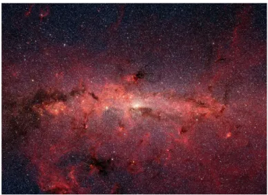
Figure 1.1: Mosaic of the GC taken by the Spitzer’s Infrared Array Camera (IRAC) showing a few 10

stars. In the optical, the extinction by dust hides the GC. This is a false-color image.

Blue: 3.6 µm, green: 4.5 µm, orange: 5.8 µm, and red: 8.0 µm. Therefore the cool and old stars are in blue and the hot dust is shown in red. Both bright and dark filamentary clouds can be seen. The brightest white spot in the middle of the image is the very center where the SMBH is located. The scale of the image is ∼ 273 pc × 196 pc. Image credit: NASA, JPL-Caltech, Susan Stolovy (SSC/Caltech) et al.

1.1.2 The Dynamical Components of the Galactic Center

The SMBH dominates the gravitational potential inside its radius of influence r

of about 3 pc. The radius of influence is the radius where the gravitational potential of the SMBH without the stars is equal to the gravitational potential of the nucleus without the SMBH, i.e. −GM

/r

= φ

(r

). If we consider a singular isothermal distribution for the nucleus with a stellar mass density of ρ

= σ

/2πGr

and with a constant velocity dispersion of σ

, then the radius of influence is r

= GM

/σ

. Studying the stars well outside the radius of influence of the SMBH (100 pc scale) can define the boundary conditions for the inner GC; this means that they can play the role of the control sample for distinguishing the effects of the SMBH from the stellar phenomena.

The GC is the center of the Galactic bulge with a typical length scale of ∼2 kpc. It

is made of an old (∼10 Gyr) stellar population. Further out of the radius of influence

of the SMBH, the star-forming region of the Milky Way (100–200 pc) is located

(Figer et al. 2004). The star formation is most likely fed by the sizeable reservoir of

molecular gas, the central molecular zone in the inner ∼200 pc (Serabyn & Morris

4 CHAPTER 1. INTRODUCTION

1996). Thus the population of the GC is a mixture of the old bulge, intermediate-age, and young stars from recent star formation epochs (Philipp et al. 1999; Mezger et al.

1999; Figer et al. 2004). Half of these young stars are in three young (. 5 Myr) clusters: The Quintuplet with projected distance of ∼ 30 pc away from the center, the Arches also with projected distance of ∼30 pc away, and the central cluster around the SMBH (Figer 2003).

The radius of influence of the SMBH in the GC is as far as 3–5 pc (see Fig. 1.2, Alexander 2005, 2011). There is very little gas within this radius. Beyond the influence of Sgr A*, 10–100 pc, there are a few 10

stars, giant molecular clouds (GMCs) and young binaries (Perets et al. 2007). At the border of the radius of influence (∼1.5–4 pc) there is a ring of dense molecular cloud streamers called circum-nuclear disk (CND). The CND (with a mass of a few 10

M , Becklin et al.

1982; Güsten et al. 1987; Herrnstein & Ho 2002) and a three-armed structure called Sgr A West (also known as the "mini-spiral") are bordered by a young supernova remnant, Sgr A East (see Fig. 1.3) and surrounded by a number of giant molecular clouds on a scale of 5–100 pc (Güsten & Downes 1980; Mezger et al. 1996). The inner 0.5 pc is made of low-mass red and massive blue giants (the products of recent star formation Bartko et al. 2010), and low-mass main sequence stars (B-dwarfs).

The existence of fainter main sequence stars and compact remnants, i.e. white dwarfs (WD), neutron stars (NS), and stellar black whole, is presumed. The red giants and the B-dwarfs have an isotropic distribution while blue giants (a few 100 massive OB stars) are in one or maybe two warped and rotating disks (Levin &

Beloborodov 2003; Genzel et al. 2003). There is a sharp cut off of their distribution at 0.04 pc. In the inner 0.04 pc (1 arcsec) the distinct S-cluster exists, which is consisting of mostly B-dwarfs (main sequence B-stars) on isotropic orbits (see 1.4).

The distribution of the low-mass faint main sequence stars, dark stellar remnants, and particularly a few tens of sollar mass stellar black holes (the "dark cusp") below the current detection limit is unclear.

The SMBH at the GC is at the lower limit of the SMBH masses detected so far (Kormendy & Ho 2013). The supermassive black holes with masses M

. 10

M

are expected to be enveloped by a dense dynamically relaxed cusp of old stars in keeping with the observed M

–σ relation for the mass of the black hole and the velocity dispersion of the spheroid of the host galaxy (Ferrarese & Merritt 2000;

Gebhardt et al. 2000). The only directly detectable tracers of the faint old population are the red giants (K magnitude . 16). The observed distribution of the red giants in a core inside ∼0.5 pc at the GC is flat or even dip instead of rising towards the center (Do et al. 2009; Buchholz et al. 2009; Bartko et al. 2010). The cusp is mainly composed of massive young stars. The reason of it is puzzling and unclear. One explanation could be that some selective mechanism destroys (Amaro-Seoane &

Chen 2014) or rejuvenates the old stars so that they apear as hot stars (Hansen &

Milosavljevi´c 2003). So far none of these proposed mechanisms are plausible and a in situ star formation is favorable (Alexander 2005). An alternative explanation is that there is no cusp and the GC is not relaxed. A major perturbation that ejected the stars from the GC would increase the relaxation time beyond the Hubble time.

Therefore the GC is still returning to its equilibrium through the 2-body relaxation (Merritt et al. 2010). A galactic merger could be such a perturbation (Milosavljevi´c et al. 2002). However there is no other indication of such a major merger.

Scenarios have been suggested to describe the existence of young stars through

1.1. THE GALACTIC CENTER 5

S-cluster

Warped Disks

Molecular Clumps

0.04 pc

2 pc 1.5 pc

0.5 pc

Figure 1.2: Not-to-scale schematic of the GC showing the dynamical components close to Sgr A*. The stars are shown with small circles. The colours show their spectral types; dark red: red giants, dark blue: blue giants, and light blue: B-dwarfs. Blobs show the gas clouds.

The large black circle in the center is the SMBH.

star formation (Morris 1993; Morris et al. 1999; Genzel et al. 2003; Levin &

Beloborodov 2003; Milosavljevi´c & Loeb 2004; Nayakshin & Cuadra 2005), although

strong tidal interactions with the SMBH should suppress star formation in the central

region. As an example, Jalali et al. (2014), using hydrodynamic simulations, shows

that the strong orbital compression of the molecular clumps existing in the CND in

their highly eccentric orbits about the SMBH, increases the gas densities to values

higher than the tidal density of the SMBH. Therefore, star formation can occur

near the SMBH. IRS 13N, located 0.1 pc away from the SMBH at the GC, which

consists of young stellar objects (YSOs) with ages of less than a million year, can be

an example (Eckart et al. 2004, 2013; Muži´c et al. 2008). Another possibility to

explain the existence of young stars in the central ∼ 0.5 pc is an inspiraling cluster

scenario (Gerhard 2001). However, this scenario is unlikely, since the tidal field of

the SMBH can disintegrate even a dense stellar cluster before reaching the center

unless it is held together by an intermediate black hole (IMBH; with a M

between

100–10

M ) (Hansen & Milosavljevi´c 2003). So far there is no evidence of the

existence of an IMBH in the GC. Moreover, there is a steep cut off in the distribution

of the young stars at ∼0.5 pc and there is no tidal tail of stripped stars (Paumard

et al. 2006), which is expected in this scenario. In general, the in situ fragmenting

gas disk scenario is more in favor of the observations and modeling.

6 CHAPTER 1. INTRODUCTION

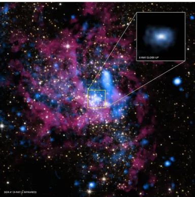
Figure 1.3: Multi-wavelength image of the GC containing the X-ray emission from the Chandra telescope in blue and the infrared emission from the Hubble Space Telescope (HST) in red and yellow. The inset is Sgr A* in the X-ray, covering a region of ∼0.15 pc wide. The diffuse X-ray emission is from the hot gas captured by the black hole and being pulled inwards. Image credit: X-ray: NASA/UMass/D.Wang et al., IR: NASA/STScI

1.1.3 The S-cluster

In the inner ∼0.04 pc of the GC, there is not any bright giants and only a population of faint blue stars are observed, which are known as the "S-stars" or "S-cluster" after their identifying labels.

Studying the S-cluster, by means of fitting Keplerian orbits to their motion is the most powerful evidence for the compactness of the central dark mass. The optimum band for the observation of these stars is ∼2.2 µm, where the extinction is less than 3 mag. Using adoptive optics at the 8m-class telescopes, the intrinsic resolution of the instrument is ∼50 mas, which enables the measurements of stellar orbits with semimajor axes of similar sizes corresponding to an orbital period of a few tens of years. The proper motion of the S-stars was presented by Eckart &

Genzel (1996) for the first time and soon after the orbits of a handful of stars were determined (Eckart & Genzel 1997; Ghez et al. 1998; Schödel et al. 2002, 2003;

Ghez et al. 2005; Eisenhauer et al. 2005a). Before long, the orbits of more than

1.1. THE GALACTIC CENTER 7

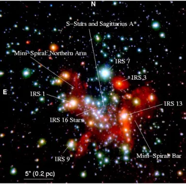
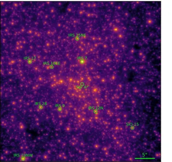
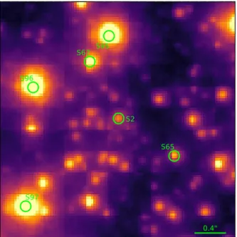
Figure 1.4: Central parsec of the GC, using the NIR camera and adoptive optics system of NACO/European southern observatory (ESO) VLT. The images of H, K, and L

band (at

2.18 µm, 2.36 µm, and 3.8 µm) were combined to obtain a pseudo-color image. Image credit:

University of Cologne.

twenty stars were fully known (Gillessen et al. 2009b; Meyer et al. 2012; Boehle et al. 2016). Up until now, 84 stars ranging from S1 to S175 (plus R34 and R44) are found to be associated with the S-cluster and the number of the determined stellar orbits (including some of the disk members) in the central ∼ 1 arcsec is about forty (Gillessen et al. 2017). Figure 1.5 shows seventeen of these determined orbits.

Most of these forty stars (thirty two of them) are on randomly oriented orbits with a thermal eccentricity distribution (members of the S-cluster). Thirty of these are spectroscopically confirmed early-type stars (the remaining two have unknown spectral type, i.e. S39 and S55/S0-102) and the rest are late-type stars (S17, S21, S24, S38, S85, S89, S111, S145). Among the forty stars with determined orbits, eight stars have been identified as members of the stellar disk (S66, S67, S83, S87, S91, S96, S97, and R44, Yelda et al. 2014).

The members of the S-cluster are main sequence B-stars with a few tens of sollar masses, which are sometimes naively associated with the young stars farther out.

However, they are considerably different from the young disk stars. The disk stars

are on approximately circular co-rotating orbits while the S-stars are on randomly

8 CHAPTER 1. INTRODUCTION

oriented elliptical (higher eccentricity) orbits. Furthermore, the S-stars are early B- stars while the disk stars are bright massive O-stars. The brightest S-stars are much fainter and long-lived than the young disk stars. Some authors have considered a disk origin for the S-stars (Milosavljevi´c & Loeb 2004; Löckmann et al. 2009;

Madigan et al. 2009; Griv 2010) but they do not provide a compelling scenario for the inverse mass segregation, where the lower mass stars are more to the center than the massive stars.

A proposed scenario to explain the origin and nature of the S-stars is that they migrated to the central arcsec from the field (outside of the central parsec), so they are unassociated to the disk stars. But as it is already discussed above, migration scenarios are not conclusive. Another interesting suggested scenario is the dynamical capture of binaries travelling to the center by the SMBH tidal disruption (Hills 1988). Such binaries are scattered in parabolic orbits and the point of the tidal disruption becomes the periapse distance for the captured star.

This could additionally unravel the origin of the hypervelocity stars (HVSs) in the Galactic halo (Perets 2011). There is a number of evidence to reinforce this suggestion. One is the luminosity function (LF) of the S-stars, which is similar to the one observed in the field and is different from the flat LF of the disk stars (Genzel et al. 2010). Another evidence is the high eccentricity of the S-stars, which is not expected from an isotropic distribution (Gillessen et al. 2009b). Also, the number of the observed S-stars (∼ forty) is consistent with the number of the HVS (see Brown 2015). However, the 2-body relaxation is not fast enough to divert the massive binaries from the field to the center to maintain the number of the S-stars.

An explanation can be the existence of massive perturbers (GMCs) in the distance of ∼5–100 pc (Perets et al. 2007).

Not long ago, a fast-moving infrared excess source within the cluster has been discovered on a highly eccentric orbit towards the black hole (Gillessen et al. 2012).

Strong evidences suggest that this source, called the Dusty S-cluster object (DSO) (Eckart et al. 2013) or G2 (Gillessen et al. 2012) is a member of the cluster. Further monitoring of the DSO to detect the potential effect on the activity of the SMBH has raised many different scenarios and interpretations of the data about the nature of the source. The prime argument is whether the DSO is a dust-enshrouded star, which has kept its compact nature and is continuing its motion along the same orbital trajectory as is suggested by Eckart et al. (2013) (see also Witzel et al. 2014;

Valencia-S. et al. 2015; Shahzamanian et al. 2017; Zajaˇcek et al. 2017) or it is, as

Gillessen et al. (2012) (see also Gillessen et al. 2013a,b; Pfuhl et al. 2015; Plewa

et al. 2017) suggest, a gaseous and dusty coreless cloud of a few Earth masses,

which is tidally stretched after going through its periapse passage in 2014. Some

even suggest that the origin of the DSO/G2 is likely related to the precursor source

G1, since there is some similarities in their orbital evolution, though their orbits

are not identical (Plewa et al. 2017). The Keplerian orbital parameter of the DSO

is very well constrained (see Valencia-S. et al. 2015) and since the source seems

to be compact and still following the same orbit, the dust enshrouded scenario is

more plausible. Moreover, in the anticipation of the possible tidal disruption of a

gas cloud, many tried to observe the increased activity of Sgr A*, but no additional

activity has been observed.

1.1. THE GALACTIC CENTER 9

0.8 0.6 0.4 0.2 0.0 0.2 0.4 0.6 0.8 R.A. (") 0.6

0.4

0.2

0.0

0.2

0.4

0.6 Dec. (")

S1 S2 S4 S5 S6 S8 S9 S12 S13 S14 S17 S18 S19 S21 S22 S23 S24 S29 S31 S38 S39 S42 S54 S55 S60 S67 S71 S85 S89 S145 S175 F igure 1.5 : Best-fit stellar orbits of 31 stars around Sgr A* in the central ∼ 0

.6. The fitting procedure is done by Lauritz T izian Thomkins for 23 stars and the rest of the orbital parameters are taken from Gillessen et al. ( 2017 , T able 3).

10 CHAPTER 1. INTRODUCTION

1.2 Keplerian Orbits

For studying and modeling the stellar phenomena, in most cases the stars can be regarded as point masses dominated by the gravity. The very large difference between the mass of a star and that of a SMBH simplifies the studies as a result of negligible star-star gravitational interactions. To simplify matters, in most processes the Newtonian dynamics are sufficient and the GR effects can be neglected.

The motion of a star relative to a black hole can be expressed in a form of a Keplerian orbit, which is an ellipse, parabola, or hyperbola with a two-dimensional orbital plane in a three-dimensional space. It is a solution to a special case of a two-body problem known as the Kepler problem with three assumptions:

1. The bodies are spherically symmetric and can be treated as point masses.

2. No external or internal forces acting upon the bodies other than their mutual gravitation exists.

3. When compared to the central body, the mass of the orbiting body is insignifi- cant.

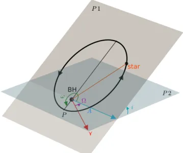
This solution can be expressed via six orbital elements known as the "Keplerian elements" (Fig.1.6). A position and velocity vector in three dimensions known as the orbital state vectors characterize the motion of an object. The orbital parameters can be obtained from the state vectors or vice versa. In contrast to the state vectors, five of the total six orbital elements are constant, which makes using the orbital elements more convenient. Two of the orbital elements define the size and shape of the orbit:

• Semimajor axis a

• Eccentricity e

Three angles (Euler angles) define the orientation of the orbital plane in three dimensions:

• Inclination i, defined as an angle between the orbital plane and the reference plane (the plane of the sky here)

• Longitude of the ascending node Ω , defined as the angle between the refer- ence direction (North within the frame of our work) and the ascending node on the reference plane

• Argument of periapse ω, defined as the angle between the ascending node and the periapse in the orbital plane

And Finally:

• True anomaly ν, defined as the position of the orbiting body along the trajec-

tory measured from the periapse

1.2. KEPLERIAN ORBITS 11

star

BH A i ω Ω

P

P 1

P 2

Figure 1.6: Keplerian orbital elements for a star revolving a black hole. Here BH is the central black hole, P1 is the orbital plane, P2 is the plane of the sky, g is the reference direction, A is the ascending node, P is the periapse, i is the inclination, ω is the argument of periapse, and Ω is the longitude of the ascending node.

There are several alternatives to the true anomaly such as the mean anomaly M or the time of the periapse passage T

.

In order to find the position of a star at each epoch, "Kepler’s equation" has to be written and solve. The "Kepler’s equation" is defined as:

M = E − esinE, (1.1)

where E is the eccentric anomaly. Eccentric anomaly is the angle that defines the position of a body on a Keplerian orbit, while mean anomaly M is an angle in an imaginary circular orbit corresponding to the eccentric anomaly. M and e are known parameters, and the equation has to be solved for E. However, since sine is a transcendental function, there is no algebraically solution to the equation. This means that the approximate value of E has to be found numerically by finding the root of the following equation iteratively

f (E) = E − esinE − M. (1.2)

12 CHAPTER 1. INTRODUCTION

One possibility is to use the Newton’s method (also known as the Newton–Raphson method). The method starts with f(E), the derivative f

(E), and an initial value E

as an approximate solution. In this case, the initial value of E

= M is sufficient.

However, for e > 0.8, E

= π should be used. A better approximation is determined by

E

= E

− E

− esinE

− M 1 − ecosE

. (1.3)

The iteration is continued until a desired accuracy is obtained. The idea behind this method is that if the initial guess is close enough to the solution, then its tangent line approximates the function. The intercept of this tangent line is a better approximation to the solution than the initial guess. If the initial guess is close enough to the solution and the derivative at the initial value exist, the method will usually converge. The rate of convergence is quadratic, if the multiplicity of the root is 1, similar to the case here. Otherwise, the convergence rate is linear. There is a method to preserve the quadratic convergence rate in these cases.

1.3 General Relativity and Black Holes

General relativity is the geometric theory of the gravitation by Albert Einstein in 1915 (Einstein 1915). It provides a unified description of the gravity by generalizing special relativity and the Newton’s law of gravitation as a geometric property of the space-time. The relation of the curvature of the space-time to the energy and momentum of the matter and radiation is specified by the Einstein field equation, which is a system of ten partial differential equations in the form of a tensor equation. The solution to these equations is the components of the metric tensor for a given stress-energy in the space-time. The trajectory of the particles, with mass or massless (photons) are then calculated using the geometric equations. General relativity predicts that a sufficiently compact mass can affect the space-time to form a black hole. However, the idea of a massive body that even light cannot escape from it was already proposed by John Michell. A few months after the development of GR, Karl Schwarzschild found a solution to the Einstein field equation, which describes a static black hole (Schwarzschild 1916). During the golden age, other solutions to the Einstein field equation for the charged (Reissner 1916; Nordström 1918), spinning (Kerr 1963) or spinning and charged (Newman et al. 1965) black holes were found.

General relativity has been tested by many different experiments, from the Eddington’s solar eclipse expedition in 1917 to the modern observations of the binary pulsar systems. However, all these tests are in the weak-field regimes, while general relativity is untested in the strong-field regime. Near-infrared observations of the stars and pulsars are tests of the weak-field regime (r r

) too. In this regime, using a parametrized post-Newtonian (PN) formalism with the Newtonian gravity is sufficient, while for the strong-field regime (r ∼ r

) tests such as the observations of the accretion flow, careful modeling of the space-time is needed.

The tests of GR with the gravitational wave observations of the extreme mass-ratio inspirals (EMRIs) are also in this regime.

Black holes have no "hair". According to the "no hair" theorem, black holes are

1.3. GENERAL RELATIVITY AND BLACK HOLES 13

uniquely described by the three parameters of the Kerr-Newman metric, namely the mass, angular momentum, and electric charge. All other information about the matter inside the black hole (or "hair") vanishes behind the event horizon. An event horizon is a virtual boundary that disconnects the interior of a black hole from the its exterior. General relativity has predicted the existence of the event horizon, but there has been no proof of it so far. Other important physical properties of a black hole are the singularity (where the spacetime curvature becomes infinite) and photon sphere (a spherical boundary where any photon with a tangent motion would be trapped in a circular orbit). It can be argued that an astronomical black hole can be described by the Kerr metric since black holes are believed to be the final state of the evolution of massive stars and during their formation any other signature other than the mass and spin of the original star is radiated away.

Moreover, astrophysical black holes are thought to be basically electrically neutral as a result of neutralization of any residual electric charge.

1.3.1 Post-Newtonian Approximation

The post-Newtonian (PN) approximations are used to find an approximate solution of the Einstein field equation for the metric tensor. These approximations are expanded in small parameters, for example, the ratio of the velocity of matter to the speed of light (v/c), which express the orders of deviations from the Newtonian gravitation in the weak-field region. Higher order terms are added for more accuracy.

If the small parameter used for the expansion is zero, the PN approximations reduce to the Newtonian law of gravity.

The simplest black hole that has a mass but neither a charge nor spin is called a Schwarzschild black hole. There is no observational difference between the gravitational field of this type of black hole and any other spherical object with the same mass. The event horizon of the Schwarzschild black hole is called the Schwarzschild radius (r

). A mass that is neither charged nor rotating and is smaller than its Schwarzschild radius, forms a black hole. Since the precession of the orbit of a test particle due the frame-dragging near a rotating black hole is very small, to find the orbit, an astrometric black hole can be considered to be a Schwarzschild black hole for simplification. A Schwarzschild black hole is described by the Schwarzschild metric. The line element of the Schwarzschild metric has a form of

c

ds

= 1 − r

r

c

dt

−

1 − r

r

dr

− r

dθ

+ sin

θdφ

. (1.4)

Here r

is the Schwarzschild radius defined as 2GM/c

(Schwarzschild 1916). A particle orbiting in this metric can have a stable circular orbit with r > 3r

. A circular orbit of minimum radius 1.5r

, corresponds to an orbital velocity approaching the speed of light (c). A star that is sufficiently close to a Schwarzschild black hole experiences an acceleration given by equation

a

= − M

~ x r

+ M

~ x

r

4 M

r − v

+ 4 M

r ˙

r

~v, (1.5)

in the first PN order, where ~ x and ~v are the position and velocity vector of the

star and G = c = 1 (Will 1993). The numerical integration of this equation will

14 CHAPTER 1. INTRODUCTION

result in the elliptical orbit of the revolving star showing precession in the orbital plane. Using a Kerr-Newman black hole instead of a Schwarzschild one, will add a few more terms due to the angular momentum vector (the frame-dragging effect) and quadruple moment of the black hole (see for examples, Zhang et al. 2015;

Johannsen 2016; Will & Maitra 2017; Zhang & Iorio 2017; Iorio & Zhang 2017;

Hees et al. 2017; Iorio 2017).

The relativistic parameter at periapse is defined as Υ ≡ r

/r

with r

being the Schwarzschild radius and r

the periapse distance. The relativistic parameter changes along the orbit. A mildly relativistic orbit follows an almost Keplerian energy equation and Υ can be expressed as

Υ = β

+ GM

c

a ≡ β

+ Υ

. (1.6)

Here a is the semimajor axis and β ≡ v/c (Alexander 2005). If e 0 and the star is close to its periapse, then β

Υ

and consequently Υ ∼ β

. The deviations from the Newtonian mechanics become greater as Υ increases. For Υ 1, which is the case for the stars near the SMBH at the GC, it is advantageous to expand the PN deviations in β and attribute each effect by the order of its β-dependence or equivalently, by the orders of r

/r

or r

/a (Alexander 2005).

1.3.2 Relativistic Interactions with a Supermassive Black Hole When a star approaches a SMBH on an orbit with a periapse distance smaller than the tidal disruption radius of the black hole, the work done by the tidal field transfers the energy and angular momentum from the orbit of the star to the star itself and unbinds it (Alexander 2017). Therefore, the observable relativistic interaction near a SMBH depends on the tidal radius to event horizon ratio. A

∼1 M main sequence star will be disrupted outside the event horizon of a SMBH and the tidal interactions perturb its motion outside the tidal disruption radius.

However, stellar black holes and to some extent the NSs and WDs can reach the event horizon without perturbations. Consequently, the main sequence stars can merely be the probes for the weak PN effects, while stellar remnants can be probes for the strong gravity.

The observed redshift curve z(t) can be expanded in terms of β in three- dimensions (Alexander 2005; Zucker et al. 2006),

z = ∆λ

λ = B

+ B

β + B

β

+ O(β

). (1.7) Two effects contribute to the second term, the special relativistic transverse Doppler effect and the GR gravitational redshift. The GR gravitational redshift, which also contributes to the zeroth-order z expansion, is

z

= (1 − r

/r)

− 1 ' r

/2r = r

/4a + β

/2, (1.8) and the relativistic Doppler shift of a moving source seen by an observer at rest is

z

= 1 + βcos(v)

p 1 − β

− 1 ' βcos(v) + β

/2, (1.9)

1.3. GENERAL RELATIVITY AND BLACK HOLES 15

where v is the angle between the velocity vector and the line of sight (Alexander 2005; Zucker et al. 2006). The first order term is the Newtonian Doppler shift and the second order term is the special relativistic transverse Doppler effect. The lowest order β

effects, which are already above the detection limits of the current instruments through spectroscopy (Zucker et al. 2006) are expected to be observed in the near future.

Another effect that needs to be considered here is the Roemer delay. It is a Newtonian effect and caused by the fact that the travel time for the light coming from a star to the observer changes with the orbital phase, when the orbit has an inclination with respect to the plane of the sky. This difference between the emission and arrival times of the signal causes a deviation from a Newtonian orbit, which is dependent on the orbital parameters. The Roemer effect is also a β

correction, which is larger than both the GR gravitational redshift and the Special relativistic transverse Doppler effect. Multiple stars and their proper motions are needed to break this degeneracy.

The third-order (β

) GR effects, such as the frame dragging

, gravitational lensing

of the background stars by a SMBH and stellar black holes (Alexander &

Sternberg 1999a,b; Alexander 2001), and Shapiro delay

(Shapiro 1964; Kopeikin

& Ozernoy 1999), or GR periapse shift (although it is a β

effect in the proper motions) will not be detectable with the available radial velocity data.

There are some debates over whether the relativistic precession in the proper motion of the known short period stars is observable with the current instruments.

There is a high expectation for the detection of these effects and the no-hair theorem (Will 2008; Merritt et al. 2010; Iorio 2011; Zhang et al. 2015) on the very short period stars by the IR interferometer GRAVITY (Eisenhauer et al. 2011). However, the Newtonian precession and resonant relaxation perturbations by the background stars can partially or completely affect the detection of the relativistic precessions (Merritt et al. 2010; Sabha et al. 2012). Nevertheless, it is unclear how many of these relativistic stars are in short orbits around the SMBH. High precision measurements of the radio pulsars could give us a better understanding of the properties of the SMBH (Eatough et al. 2015), but so far there is only one pulsar detected near Sgr A*. The observation in the GC increased after the discovery of the DSO/G2. This led to the discovery of a pulsar 0.12 pc away from the black hole after the very bright flare recorded by Swift in April 2013 (Kennea et al. 2013). The NuSTAR X-ray telescope reported that the flaring object is a magnetar with a spin rate of 3.76 seconds (Mori et al. 2013). Observing the gravitational lensing of the background stars by the SMBH and stellar black holes is also anticipated (Alexander

& Sternberg 1999a,b; Alexander 2001). Gravitational lensing of the stars by the SMBH is slightly different from the other effects discussed here, since it is an effect on the light emitted by a star, rather than an effect on the star itself, and since the affected stars are usually far away from the dynamical radius of influence of the

1

The changes in the trajectory of a star orbiting a spinning black hole by changes in the longitude of the ascending node corresponding to the precession of the orbital angular momentum vector around the black hole’s spin vector, also known as the Lense-Thirring precession.

2

The bending of the light from the source by a distribution of matter (called the gravitational lens) such as a cluster of galaxies or a black hole, as it travels towards the observer.

3

Radar signals passing near a massive object take slightly longer to travel to a target and longer to

return. The time delay is caused by the spacetime dilation, which increases the path length. The Shapiro

time delay is one of the four classic solar system tests of GR.

16 CHAPTER 1. INTRODUCTION

SMBH. Another class of the GR effects that may also be detectable in the GC is the emission of the gravitational wave (GW) from the very low-mass stars that spiral into the SMBH.

The strong interactions of stars with a SMBH, defined as interactions, indescrib- able by the Newtonian gravity, such as the annihilation or absorption of the whole star by the SMBH or the tidal disruption are beyond the scope of this thesis.

1.4 Observation and Data Reduction 1.4.1 Observations

Figure 1.7: VLT in the Paranal observatory, Chile. Image credit: John Colosimo/ESO.

In astronomy, the infrared range is divided into three subcategories of near-infrared (NIR): ∼0.7–5 µm, mid-infrared (MIR): ∼5–30 µm, and far-infrared (FIR): ∼30–

1000 µm. For observations in the mid to far-infrared regimes using rockets, balloons, aircrafts, and space telescopes are necessary, since some bands get absorbed fully by the atmosphere. In order to be able to observe in the NIR, ground-based telescopes have to be in dry locations in high altitudes, since there will be less water vapor absorption in the atmosphere. The very large telescope (VLT) is located in such a condition in Cerro Paranal, 2635 metres above the sea level in the driest desert on Earth, Atacama in Chile. The VLT consists of four unit telescopes (UT) with 8.2 m primary mirrors, which can work together as an interferometer called the VLTI. For the purpose of this work, one unit telescope has been used. There are also four movable auxiliary 1.8 m telescopes as can be seen in Fig. 1.7. The location of the VLT is ideal to study the GC since it is mostly visible from the southern hemisphere.

Since the GC is a very crowded region and Sgr A* is a very faint source in the NIR, a high angular resolution is needed in order to distinguish the sources and locate the black hole.

In this work, K

-band (central wavelength 2.18 µm with width of 0.35 µm)

images of the central cluster are acquired with the NACO instrument, which is

reinstalled from 2014 in the UT1 of the VLT. It was installed before in the UT4 from

2001 to 2013. The NACO instrument is a combination of the Nasmyth adaptive

optic (AO) system (NAOS) and the Coude near-infrared camera (CONICA). NAOS

is designed to work with natural guide sources. CONICA is a NIR imager and

1.4. OBSERVATION AND DATA REDUCTION 17

spectrograph capable of AO assisted imaging, no AO imaging, imaging polarimetry, and cornography. The characteristics of the cameras of CONICA are described in Table 1.1 in terms of the plate scale and field-of-view (FoV).

Table 1.1: CONICA list of cameras. Credit: ESO NACO user manual.

Camera Scale FoV Spectral Range

(mas/pix) (arcsec) (µm)

S13 13.221 ± 0.017 14 × 14 1.0 – 2.5 S27 27.053 ± 0.019 28 × 28 1.0 – 2.5 S54 54.50 ± 0.10 56 × 56 1.0 – 2.5

L27 27.19 28 × 28 2.5 – 5.0

L54 54.9 56 × 56 2.5 – 5.0

1.4.2 Adaptive Optics

Reaching the diffraction-limited resolution in a telescope is not possible due to the atmospheric turbulence and instrumental effects of the telescope itself. Ideally, the angular resolution of the telescope is given by θ = 1.22λ/D. The parameter D is the diameter of the primary mirror of the telescope and λ is the observing wavelength. For the VLT, the diffraction-limited resolution at λ = 2.2 µm is 0

.057.

The atmospheric turbulences limit this resolution to λ/r

∼ 0

.7. The effecting parameter here (r

) is the Fried parameter, which is related to the strength of the turbulence and is dependent on the wavelength by λ

. The correlation time of the turbulence t

is another effecting parameter, which is related to r

and the speed of the turbulent air, and corresponds to the time-scale over which the changes in the turbulence become significant. In order to have stable atmospheric conditions and a better performance of the AO system, these two parameters, i.e. r

and t

, have to be sufficiently large. The "seeing" can be described by these two parameters as = 0.98λ/r

(Fried 1966). Moreover, heat, wind force, and gravity cause deviation in the telescope structure, which leads to image degradation.

Adaptive optics system can correct for all these small changing errors and compensate in the real-time for the deformation of the wavefront (WF) caused by the atmospheric turbulence on a bright guide star. The incoming light is split by a dichroic mirror and travels to a wavefront sensor (WFS). The WFS and a Real-Time Computer (RTC) that processes these measurements and controls a deformable mirror (DM) to correct for them and restore the WF flatness then measure the distortions in the WF. The DM is a thin plate mirror placed on a set of piezoelectric actuators that can push and pull it from the back. The DM of NAOS contains 185 actuators. The quality of the image is determined directly by the WF error. The seeing parameter r

determines the spacing of the actuators needed in an AO system and t

determines the correction speed required to compensate for the effects of the atmosphere. An AO system works in a closed loop. The DM flattens the WF and the WFS measures the residual WF error. A schematic view of the AO system is shown in Fig. 1.8.

An important parameter that defines the image quality is the Strehl ratio (SR). It

corresponds to the ratio between the intensity peaks of the corrected image and the

18 CHAPTER 1. INTRODUCTION

Figure 1.8: Principle of the Adaptive Optics. Credit: ESO NACO user manual.

theoretical point spread functions (PSFs); i.e. a higher ratio corresponds to a better image quality. For the GC observations, the bright supergiant IRS 7 (with a K

-band magnitude of ∼7), which is located ∼5

.6 north of Sgr A* is a good candidate for guiding star. Since finding the proper guiding source is not always trivial, there is an alternative method called the laser guide star (LGS) technique. In this technique, an artificial guiding point source is created by a Sodium-laser that excites the Sodium atoms in the mesosphere at 90 km altitude. If the observing conditions are suitable and the guide star is a close and bright source, the resulted PSF will be very close to the diffraction limit. In this situation, the Strehl ratio in the K

-band will be more than 30%. In the case of not suitable observing conditions or at shorter wavelengths, the Strehl ratio is only a few percent. The current AO systems correct images at λ > 1 µm since for shorter wavelengths higher computational power is needed.

1.4.3 Data Reduction

Several adverse effects caused by the detector itself or by the thermal emission

of the telescope or the sky emission at that special wavelength can influence the

image. Therefore, it has to be corrected. The detector has inhomogeneity from its

production procedure or from ageing. As a result, a given flux of the photons can

be recorded by different counts at a different region of the detector. In order to

correct for this issue, it is necessary to get the detector’s response function on the

night of the observation. To do so, a map of the pixel response is produced by the

images of the twilight sky (the sky flat-field) or a lamp (the lamp flat-field), when

the lamp is switched on and off. The on/off images of the lamp are then subtracted

and averaged. The object frame is then divided by the flat-fields, which is called

flat-fielding. Another method that also can minimize the detector’s cosmetics is

1.4. OBSERVATION AND DATA REDUCTION 19

jittering. The idea is to not let the sources lie on the same position of the detector.

Taking several images of the field with offsets of small values does this.

The sky frame has to be subtracted from the object frames in order to remove the OH emission of the atmosphere for λ ≤ 2.2 µm. This is called the sky-subtraction.

The sky frame has to be taken in a nearby field to the source, where there are not any apparent sources. For the GC, the closest location is 713

west and 400

north of IRS 7. The sky frames have to be taken several times since the thermal emission changes. For λ ≤ 2.2 µm the sky observations are done every ∼2 hours while for the longer wavelengths where the atmospheric and telescope emissions are stronger, the smapling has to be done more frequently.

Replacing the dead/bad pixels with interpolations, i.e., average values, of the neighbouring pixels, does the dead/bad pixel correction. These pixels have either a zero or a high response value compared to the neighbouring pixels. Finally, the reduced images are shifted and stacked in a cube to get a mosaic image of the object or the field, in order to have higher signal to noise ratio.

1.4.4 Deconvolution

In an ideal case, the PSF, which is the image of a point source, would be an Airy pattern as a result of the diffraction of the light on the telescope aperture. In a real case the PSF varies with time due to the atmospheric turbulence and some effects of the telescope. Moreover, the PSF varies over the FoV. A deconvolution is a process used to reverse the effects of the convolution on the observed image. The observed image I( x, y) is the convolution of the real object O(x, y) with a PS F( x, y). In reality there is also an additional noise c(x, y),

I(x, y) = PS F(x, y) O(x, y) + c(x, y). (1.10) Here we wish to recover O(x, y), the real object. The symbol is the convolution operator. If we neglect the noise term, the Fourier transformation of the real object can be derived by a division in Fourier space like

O(u, ν) ˆ = I(u, ν) ˆ

P S F(u, ν) ˆ , (1.11)

where O(u, ν), ˆ I(u, ν), and ˆ P S F(u, ν) ˆ are the Fourier transformation of the original functions with u and ν being the spatial frequencies corresponding to the x and y coordinates.

Due to the limitations like neglecting the noise and inaccurate determination of the PSF, different methods have been developed to recover the object distribution.

Eckart et al. (2005) studies and compares different deconvolution methods. In this

work, Lucy-Richardson deconvoluted images of the GC using the S13 camera of

the NACO instrument has been used. Therefore I describe it bellow shortly. Before

using a deconvolution method, it is vital to estimate the PSF. The PSF in the GC can

be extracted individually for each source in the image using the software package

StarFinder (Diolaiti et al. 2000). The StarFinder is an algorithm for a crowded

stellar field for a semi-automatic PSF extraction and does high precision astrometry

and photometry. It estimates the initial PSF by finding the median of several isolated

20 CHAPTER 1. INTRODUCTION

and bright sources selected by the user and then continues by finding sources and repeating the PSF extraction.

1.4.4.1 Lucy-Richardson Deconvolution

The Lucy-Richardson deconvolution (Lucy 1974; Richardson 1972) is an iterative algorithm for recovering an image that has been blurred by a known PSF and allows for the separation of flux density contributions of very close sources. First, the current estimate of the object distribution O

(x, y) is convolved with the PS F( x, y) as

I

(x, y) = O

( x, y) PS F(x, y). (1.12) Then the resulting image I

(x, y) is compared with the observed image I (x, y),

Q( x, y) = I (x, y)

I

(x, y) PS F(x, y). (1.13)

The PSF behaves as a low-pass filter that decreases the contribution of high spatial frequencies on the result as these frequencies are strongly under the influence of the noise. Finally, a new estimation of the object distribution O

(x, y) is found by the multiplication of the old object distribution O

(x, y) by Q(x, y) as

O

(x, y) = O

(x, y) Q(x, y). (1.14) The high spatial frequencies are subdued due to the convolution with the PSF and consequently the noise amplification is prevented. A sufficient number of iterations are needed to resolve the details of the image related to the high spatial frequencies. This results in a large computation time and therefore is a drawback of this algorithm. However, the image will not always benefit from a large number of iterations, since there is a chance that the diffuse background resolves into the point sources. The addition of the diffuse background and the flux densities of very faint sources into the flux density of a bright source is also another difficulty.

Figure 1.9 shows the effect of the Lucy-Richardson deconvolution on an image of the central region of the GC.

1.5 Dissertation Outline

In this thesis, I study the physics in the vicinity of a SMBH through the observations of the S-cluster. I use the NIR imaging and spectroscopy data of the three S-stars closest to Sgr A* to determine the following:

• The mass of and the distance to Sgr A*. I start with the details of the

observations in the NIR, the data reduction, and the Newtonian and relativistic

PN models in Chapter 2. I discuss the astrometric accuracy that I can achieve

with the data and find the astrometric positions of the three candidate stars,

i.e., S2, S38, and S0-102/S55. I find the best orbital fits and consequently, I

obtain the gravitational potential parameters.

1.5. DISSERTATION OUTLINE 21

S1 S4 S2

S5 S6

S7

S8 S9 S10

S11

S12

S13 S14

S17

S18 S19

S20

S21

S22 S23

S24 S25 S26

S27 S28

S29 S30

S31

S32 S33

S35 S34

S36 S37

S38 S39

S41 S42

S43

S44

S46 S45 S47 S48

S50 S51 S52

S53

S54 S55 S56

S57

S58 S59

S60

S61 S62 S63

S64

0.2"

Figure 1.9: K

-band image of the central arcsec of the GC taken in May 2011 with the S13 camera of the NACO instrument at the VLT after the Lucy-Richardson deconvolution. The S-stars are marked by their names. The position of Sgr A* is marked by a yellow plus.

• The PN effects observable in the proper motion of S2. I develop methods that use the deviations from a Newtonian symmetric orbit to measure the PN effects within the weak-field limit in Chapter 3. S2 is the only S-star with a small enough periapse distance that makes the observation of these effects promising. It is also the only star with enough available astrometric and radial velocity data. I start with simulating the orbits of stars that are located within the orbit of S2 as case studies. The results from these simulations are analyzed by connecting them to the relativistic parameter at the periapse.

This is beneficial in assessing the magnitude of the PN effects. Finally, I apply the results on S2 in order to confirm the PN characteristics of the orbit.

I give a summary of the results in Chapter 4. Finally, I provide supplementary

information in the Appendix.