Near-Infrared Polarimetry and Stellar Classification in the Galactic Center

Classification in the Galactic Center

INAUGURAL-DISSERTATION

zur

Erlangung des Doktorgrades

der Mathematisch-Naturwissenschaftlichen Fakult¨at der Universit¨at zu K¨oln

vorgelegt von

Rainer Buchholz aus K¨oln

K¨oln 2011

Tag der m ¨undlichen Pr¨ufung: 07. 12. 2011

Abstract

The Galactic center (GC) is the closest galactic nucleus, offering the unique possibility of study- ing the population of a dense stellar cluster surrounding a Supermassive Black Hole (SMBH), as well as stellar and bow-shock polarization effects in a dusty environment.

The goals of the first part of this work are to develop a new method of separating early and late type stellar components of a dense stellar cluster based on intermediate band filters, applying it to the central parsec of the GC, and conducting a population analysis of this area. Adaptive optics assisted observations obtained at the Very Large Telescope (VLT, run by the European Southern Observatory, ESO) in the Near-Infrared (NIR) H-band (1.6 µm) and 7 intermediate bands covering the NIR K-band (2.18 µm) were used for this. A comparison of the resulting Spectral Energy Distributions (SEDs) with a blackbody of variable extinction then allowed to determine the presence and strength of a CO absorption feature to distinguish between early and late type stars. This new method is suitable for classifying K giants (and later), as well as B2 main sequence (and earlier) stars that are brighter than 15.5 mag in the K band in the central parsec. Compared to previous spectroscopic investigations that were limited to 13-14 mag, this represents a major improvement in the depth of the observations and reduces the needed ob- servation time. Extremely red objects and foreground sources could also be reliably removed from the sample. Comparison to sources of known classification indicates that the method has an accuracy of better than ∼ 87%.

312 stars have been classified as early type candidates out of a sample of 5914 sources. Several results, such as the shape of the K-band Luminosity Function (KLF) and the spatial distribution of both early and late type stars, confirm and extend previous works. The distribution of the early type stars can be fitted with a steep power law (β

= − 1.49 ± 0.12), alternatively with a broken power law, β

= − 1.08 ± 0.12, β

= − 3.46 ± 0.58, since a drop in the early type density seems to occur at ∼ 10”. In addition, early type candidates outside of 0.5 pc have been detected in significant numbers for the first time. The late type density function shows an inversion in the inner 6”, with a power-law slope of β

= 0.17 ± 0.09. The late type KLF has a power-law slope of 0.30 ± 0.01, closely resembling the KLF obtained for the bulge of the Milky Way. The early type KLF has a much flatter slope of (0.14 ± 0.02). These results seem to agree best with an in-situ star formation scenario, although alternatives like the inspiraling cluster scenario cannot be ruled out yet.

The second part of this work aims at providing NIR (H-, Ks-, and Lp-band) polarimetry of the stellar sources in the central parsec at the resolution of an 8m telescope for the first time, along with new insight into the nature of the known bright bow-shock sources.

Using the NAOS-CONICA (NACO) intrument at the ESO VLT in its polarimetric mode and ap- plying both high-precision photometric methods specifically developed for crowded fields along with a newly established polarimetric calibration for NACO, polarization maps covering parts of the central 30” × 30” (with different coverage and depth in the three wavelength bands) were produced. In addition, spatially resolved polarimetry and a flux variability analysis on the ex- tended sources in this region were conducted.

It has been confirmed for this larger sample that the foreground polarization mostly follows the orientation of the Galactic plane, with average values of 4.5 - 6.1 % at ∼ 26

(in the Ks-band, depending on the Field-of-View, FOV), (9.3 ± 1.3)% at 20

± 6

(H-band), and (4.5 ± 1.4)% at 20

± 5

(Lp-band, 3.8 µm). In the east of the FOV, higher polarization degrees and steeper polar- ization angles have been found: (7.5 ± 1.0)% at 11

± 6

(Ks-band) and (12.1 ± 2.1)% at 13

± 6

(H-band). p

/p

peaks at 1.9 ± 0.4, corresponding to a power law index for the wavelength de- pendency of α = 2.4 ± 0.7. These values also vary over the FOV, with higher values in the center.

This may indicate the influence of local effects on the total polarization, possibly dichroic ex-

tinction by Northern Arm dust. The relation between the Lp- and Ks-band polarization degrees

has an average of 0.7-0.8, consistent with previous measurements on a much smaller number

of sources. The polarization efficiency in the H- and Ks-band shows the expected power-law

dependency on the local extinction.

Several of the extended sources, namely IRS 1W, IRS 5, IRS 10W, and IRS21 show significant

intrinsic polarization in all wavelength bands, as well as spatial polarization patterns that are

consistent with emission and/or scattering on aligned grains as a polarization mechanism. The

bow-shock structure around IRS 21 could be separated from the central source for the first time

in the Ks-band, finding the apex north of the central source and determining a standoff distance

of ∼ 400 AU, which matches previous estimates. This source also shows a ∼ 50% increase in

flux in the NIR over several years. In addition, the Mid-Infrared (MIR) excess sources IRS 5NE,

IRS 2L, and IRS 2S have been found to show a significant Lp-band polarization that agrees

well with the scenario that these sources are lower luminosity versions of the bright bow-shock

sources.

Zusammenfassung

Das Galaktische Zentrum ist der n¨achst benachbarte galaktische Kern und bietet als solcher die einzigartige M¨oglichkeit, die stellare Population eines dichten Sternhaufens um ein super- massives schwarzes Loch zu untersuchen. Ebenso kann in dieser Region die Polarisation von Sternen und ausgedehnten Quellen wie sogenannte ”bow-shocks” studiert werden.

Das Ziel des ersten Teils dieser Arbeit war es, eine Methode zur Unterscheidung fr¨uher und sp¨ater Sterntypen eines dichten Sternhaufens basiert auf der Verwendung von Schmalbandfil- tern zu entwickeln, diese dann im zentralen Parsek des Galaktischen Zentrums anzuwenden und so die stellare Population dieser Region zu analysieren. Dazu wurden am Very Large Telescope (VLT) der Europ¨aischen S ¨udsternwarte (ESO) unter Verwendung Adaptiver Optik im Nahinfraroten aufgenommene Daten verwendet (8 Filter, davon ein H-Band Breitbandfilter (1.6 µm) und 7 das K-Band (2.18 µm) abdeckende Schmalbandfilter). Ein Vergleich der so gewonnenen spektralen Energieverteilungen mit einem Schwarzk¨orperstrahler mit variabler Ex- tinktion erlaubte es dann, das Vorhandensein und die St¨arke der CO-Absorption festzustellen, die wiederum zur Unterscheidung von fr¨uhen und sp¨aten Sterntypen dienen konnte. Diese neue Methode ist geeignet zur Klassifizierung von Riesen bis hinunter zum Spektraltyp K sowie Hauptreihensternen bis einschliesslich B2. Im zentralen Parsec weisen diese Klassen eine Hel- ligkeit von etwa 15.5 mag im K-band auf, was die untere Grenze dieser Methode darstellt. Dies stellt eine grosse Verbesserung gegen¨uber fr¨uheren spektroskopischen Untersuchungen mit einer Helligkeitsgrenze von 13-14 mag dar, sowohl in der Tiefe wie auch in der ben¨otigten Beobach- tungszeit. Extrem ger¨otete Objekte und Vordergrundsterne konnten ebenso zuverl¨assig aus der Analyse ausgeschlossen werden. Ein Vergleich mit bereits fr¨uher klassifizierten Quellen ergab eine Zuverl¨assigkeit dieser Klassifizierungsmethode von besser als ∼ 87%

312 von 5914 Sternen wurde ein fr¨uher Spektraltyp zugeordnet. Mehrere fr¨uhere Resultate, wie die Form der K-Band Helligkeitsfunktion (KLF) und die r¨aumliche Verteilung der fr¨uhen und sp¨aten Spektraltypen, konnten best¨atigt bzw. signifikant erweitert werden. Die Verteilung der Sterne fr¨uhen Typs folgt einem steilen Potenzgesetz (mit Exponent β

= − 1.49 ± 0.12), oder al- ternativ einem abschnittsweisen Potenzgesetz mit β

= − 1.08 ± 0.12, β

= − 3.46 ± 0.58, da bei etwa 10” ein pl¨otzlicher Abfall in der projizierten stellaren Dichte auftritt. Zus¨atzlich wur- den zum ersten Mal in signifikanter Anzahl Sterne fr¨uhen Typs ausserhalb der innersten 0.5 pc detektiert. Die Dichtefunktion der Sterne sp¨aten Typs zeigt innerhalb von 6” einen anderen Ver- lauf als weiter aussen: die projizierte Dichte steigt dort nach aussen hin an anstatt abzufallen, in Form eines Potenzgesetzes mit β

= 0.17 ± 0.09. Die KLF der sp¨aten Spektraltypen folgt einem Potenzgesetz mit Exponent 0.30 ± 0.01, was der im Bulge der Milchstrasse gemessenen Helligkeitsfunktion entspricht. Die KLF der fr¨uhen Typen ist deutlich flacher, mit einem Ex- ponenten von 0.14 ± 0.02. Diese Resultate scheinen am besten zu einer Sternentstehung in situ zu passen, d.h. direkt im zentralen Parsec, wobei allerdings alternative Szenarien wie das eines einfallenden jungen Sternhaufens noch nicht ausgeschlossen werden k¨onnen.

Der zweite Teil dieser Arbeit zielte darauf ab, erstmalig Nahinfrot-Polarimetrie der Sterne im zentralen Parsek mit der Aufl ¨osung eines 8m-Teleskops zu liefern, zusammen mit neuen Er- kenntnissen ¨uber die Natur der bereits bekannten hellen bow-shock-Quellen.

Unter Verwendung des polarimetrischen Modus des Instrumentes NACO am ESO VLT und unter Anwendung sowohl von hochpr¨azisen, speziell f¨ur Regionen hoher stellarer Dichte ent- wickelter photometrischer Methoden als auch einer neu etablierten polarimetrischen Kalibra- tionsmethode f¨ur NACO war es m ¨oglich, Polarisationskarten von Teilen der innersten 30” × 30”

zu erstellen (mit unterschiedlicher Abdeckung dieses Feldes in den verschiedenen B¨andern).

Zus¨atzlich wurden r¨aumlich aufgel¨oste Polarimetrie und eine Variabilit¨atsanalyse auf den aus- gedehnten Quellen in dieser Region durchgef¨uhrt.

F ¨ur diese gegen¨uber fr¨uheren Untersuchungen deutlich h¨ohere Anzahl an Quellen konnte best¨a-

tigt werden, dass die Vordergrundpolarisation gr¨osstenteils der Orientierung der Galaktischen

Ebene folgt, mit durschnittlichen Werten von 4.5 - 6.1 % bei ∼ 26

(im Ks-Band, abh¨angig von

der betrachteten Region), bzw. (9.3 ± 1.3)% bei 20

± 6

im H-Band und (4.5 ± 1.4)% bei 20

± 5

im Lp-Band (3.8 µm). Im Osten der hier untersuchten Region wurden im Mittel h¨ohere Polar- isationsgrade und steilere Polarisationswinkel gemessen: (7.5 ± 1.0)% bei 11

± 6

(Ks-Band) und (12.1 ± 2.1)% bei 13

± 6

(H-Band). p

/p

ist um 1.9 ± 0.4 verteilt, was einem Expo- nenten des Potenz-gesetzes der Wellenl¨angenabh¨angigkeit der Polarisierung von α = 2.4 ± 0.7 entspricht. Auch diese Werte variieren ¨uber das beobachtete Gebiet, mit h¨oheren Werten im Zentrum. Dies kann ein Zeichen sein f¨ur den Einfluss lokaler Effekte auf die Gesamtpolari- sation, m ¨oglicherweise durch Absorption an ausgerichteten Staubk¨ornern im n¨ordlichen Arm der Minispirale. Das Verh¨altnis zwischen Lp-Band und Ks-Band Polarisierung nimmt Werte von im Mittel 0.7-0.8 an, ein Wert der konsistent mit fr¨uheren Messungen auf einer wesentlich kleineren Anzahl von Sternen ist. Die Polarisierungseffizienz zeigt im H- und Ks-Band die er- wartete Abh¨angigkeit von der lokalen Extinktion in Form eines Potenzgesetzes.

Mehrere der ausgedehnten Quellen, IRS 1W, IRS 5, IRS 10W und IRS21, besitzen eine sig-

nifikante intrinsische Polarisierung in allen hier betrachteten Wellenl¨angenb¨andern. R¨aumlich

aufgel¨oste Polarisierungskarten dieser Quellen deuten auf Emission oder Streuung an ausgerich-

teten Staubk¨ornern als f¨ur die Polarisierung verantwortliche Mechanismen hin. Zum ersten Mal

konnte ausserdem im Ks-Band die bow-shock-Struktur um IRS 21 von der zentralen Quelle ge-

trennt werden. Der Apex des bow-shock wurde so etwa 400 AU n¨ordlich der Zentralquelle fest-

gestellt, was fr¨uheren Absch¨atzungen (basierend auf anderen Wellenl¨angen) entspricht. Weit-

erhin zeigt diese Quelle einen Anstieg ihres Flusses im Nahinfraroten um etwa 50% im Laufe

mehrerer Jahre. Im Lp-Band wurde ausserdem f¨ur die im Mittel-Infraroten sehr hellen Quellen

IRS 5NE, IRS 2L und IRS 2S eine signifikante intrinsische Polarisierung gemessen, die sehr

gut dazu passen w ¨urde, dass es sich bei diesen Quellen um weniger helle Varianten der hellen

bow-shock-Quellen handelte.

Contents

1 Introduction 13

2 The Galactic Center 15

2.1 The Nuclear Stellar Cluster . . . . 15

2.1.1 Stellar composition . . . . 15

2.1.2 Star Formation in the GC? . . . . 16

2.2 Extinction . . . . 17

2.3 Polarization . . . . 17

2.3.1 Foreground polarization . . . . 17

2.3.2 Local polarization . . . . 18

2.3.3 Polarization of GC sources . . . . 20

3 Data reduction techniques 23 3.1 Cleaning the Image . . . . 23

3.1.1 Standard procedure . . . . 23

3.1.2 Pattern removal . . . . 23

3.2 Deconvolution . . . . 24

3.3 Linear Deconvolution . . . . 24

3.4 Lucy-Richardson Deconvolution . . . . 25

4 Observations 27 4.1 General parameters . . . . 27

4.2 Intermediate band data . . . . 27

4.3 Polarimetric data . . . . 27

4.4 Imaging data . . . . 30

5 Photometry and calibration 33 5.1 Intermediate band data . . . . 33

5.1.1 Double deconvolution photometry . . . . 33

5.1.2 Primary Calibration . . . . 33

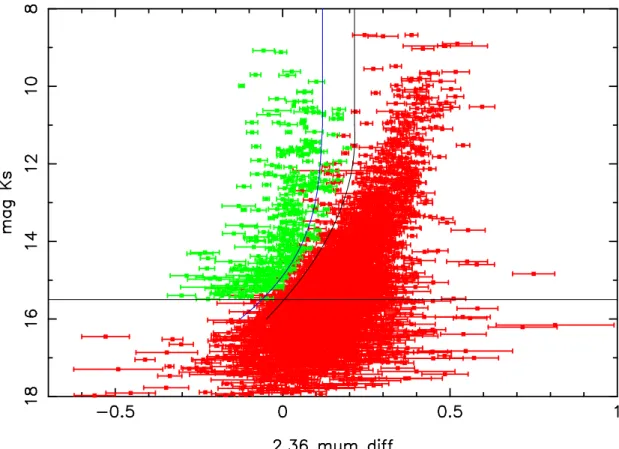
5.1.3 CO band depth as a classification feature . . . . 36

5.1.4 Cutoff determination . . . . 39

5.1.5 Local calibration . . . . 40

5.1.6 Source classification . . . . 41

5.2 Polarimetric datasets . . . . 44

5.2.1 Deconvolution-assisted large scale photometry . . . . 44

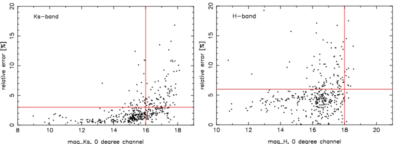
5.2.2 Error estimation . . . . 45

5.2.3 Photometry on extended sources . . . . 47

5.2.4 LR deconvolution: useful for extended structures? . . . . 48

5.2.5 Large scale aperture photometry . . . . 51

5.2.6 Polarimetry . . . . 54

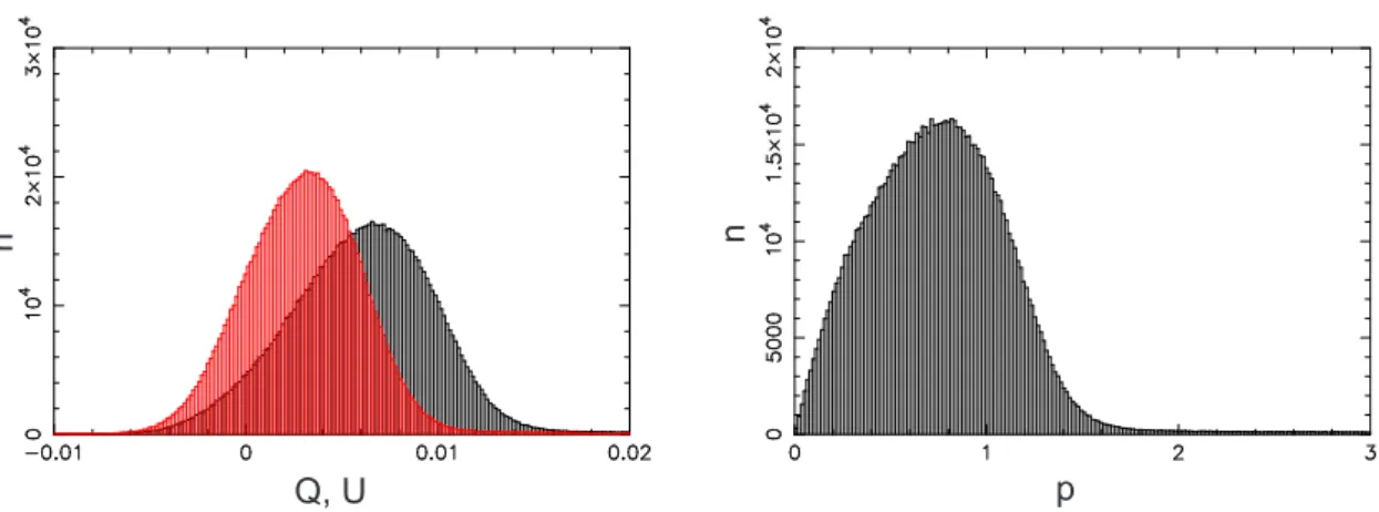
5.2.7 Calibration of the measured polarization . . . . 55

5.2.8 Correcting for foreground polarization . . . . 56

6 The stellar population in the central parsec 59 6.1 Stellar classification . . . . 59

6.2 Comparison with spectroscopic results and uncertainty estimation . . . . 59

6.3 Structure of the cluster . . . . 61

6.4 Evidence for giant depletion in the center . . . . 65

6.5 K band luminosity function . . . . 67

6.6 Extinction . . . . 68

6.7 Early type stars outside of 0.5 pc . . . . 70

7 Stellar polarization 71 7.1 Ks-band polarization . . . . 71

7.1.1 2009 data-set (P2) . . . . 71

7.1.2 2007 data-set, rotated FOV (P4) . . . . 71

7.1.3 2011 data-set (P18) . . . . 72

7.1.4 Comparing the common sources . . . . 74

7.2 H-band polarization (P1) . . . . 74

7.3 Lp-band polarization (P16) . . . . 76

7.4 Comparison to previous results . . . . 77

7.5 Comparison between the wavelength bands . . . . 80

7.5.1 H- and Ks-band . . . . 80

7.5.2 Ks- and Lp-band . . . . 85

7.5.3 Sources found in H-, Ks- and Lp-band . . . . 87

7.6 Correlation with extinction . . . . 87

8 Bow-shocks and dusty sources in the central parsec 91 8.1 Extremely red objects . . . . 91

8.2 Examining the extended sources . . . . 91

8.2.1 IRS 1W . . . . 91

8.2.2 IRS 21 . . . . 98

8.2.3 IRS 10 . . . . 103

8.2.4 IRS 5 . . . . 105

8.2.5 IRS 2 . . . . 106

8.2.6 IRS 5NE . . . . 107

9 Summary and Conclusions 109 9.1 Stellar Classification . . . . 109

9.2 Polarimetric results . . . . 111

List of Figures

2.1 Relation between emission at different NIR wavelengths . . . . 19

4.1 Ks-band field-of-view . . . . 28

4.2 Lp-band field-of-view . . . . 29

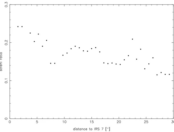
5.1 Strehl ratio over one intermediate band image . . . . 34

5.2 Primary calibration sources . . . . 35

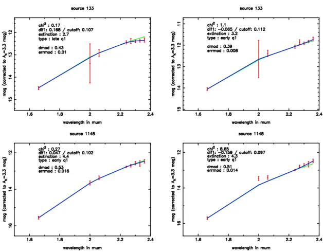
5.3 Conversion of continuous spectra into template SEDs . . . . 37

5.4 Typical Ks-band spectra of late type stars . . . . 38

5.5 CO band depth of reference sources . . . . 39

5.6 Effects of the local calibration . . . . 40

5.7 Local calibration maps . . . . 41

5.8 CO band depth of the sources in the central parsec . . . . 42

5.9 Density of stars with noisy SEDs . . . . 43

5.10 PSF polarization pattern . . . . 45

5.11 H/Ks-band flux errors (P1/P2) . . . . 46

5.12 Wiregrid flat-field Stokes parameters . . . . 47

5.13 Stokes parameter Q in flat-field with/without Wollaston prism . . . . 48

5.14 Fluxes and polarization parameters of IRS 16C (P2) . . . . 49

5.15 Fluxes and polarization parameters of IRS 1C (P2) . . . . 50

5.16 H/Ks-band lightcurve of non-variable source IRS 16C . . . . 51

5.17 Recovered polarization parameters after LR deconvolution . . . . 52

5.18 Ks-band flux errors (P18) . . . . 53

5.19 Lp-band flux errors (P16) . . . . 54

5.20 Lp-band luminosity function of detected sources . . . . 55

6.1 Stellar classification map of the GC . . . . 60

6.2 Early and late type stellar densities . . . . 61

6.3 Stellar surface density map (all stars with m

< 15) . . . . 62

6.4 Stellar surface density map (late type stars) . . . . 63

6.5 Stellar surface density map (early type stars) . . . . 64

6.6 Ks-band luminosity function of classified stars . . . . 66

6.7 Extinction map from fitted extinction values . . . . 67

6.8 Early type SEDs of outlying stars . . . . 68

7.1 Ks-band polarization map (P2,P4,P18) . . . . 72

7.2 Ks-band polarization parameters (P2) . . . . 73

7.3 Ks-band polarization parameters (P4) . . . . 74

7.4 Ks-band polarization parameters (P18) . . . . 75

7.5 Comparing the polarization of the common sources (P2/P4) . . . . 76

7.6 H-band polarization map (P1) . . . . 76

7.7 H-band polarization parameters (P1) . . . . 77

7.8 Lp-band polarization map (P16) . . . . 78

7.9 Lp-band polarization parameters (P16) . . . . 79

7.10 Polarization angle vs. polarization degree (P1,P2) . . . . 80

7.11 Relation between H/Ks polarization parameters (P1/P2) . . . . 80

7.12 Polarization parameters of pK

and pK

sources . . . . 81

7.13 Polarization parameters of pK-E and pK-W sources . . . . 82

7.14 H/Ks-band polarization parameters averaged along the East-West-axis . . . . . 83

7.15 Relation between Ks/Lp polarization parameters (P2/P16) . . . . 84

7.16 H/Ks/Lp-band polarization degrees . . . . 85

7.17 Polarization efficiency (P1,P2) . . . . 86

7.18 Polarization efficiency (P4,P18) . . . . 87

7.19 Polarization efficiency (all Ks-band sources) . . . . 89

7.20 Extinction of pK

and pK

sources . . . . 90

8.1 SEDs of Extremely Red Objects . . . . 92

8.2 Polarization map of IRS 1W (Ks) . . . . 93

8.3 Polarization map of IRS 1W (H) . . . . 94

8.4 Polarization map of IRS 1W (Lp) . . . . 95

8.5 H/Ks/Lp-band lightcurves of IRS 1W . . . . 96

8.6 IRS 21 before and after LR deconvolution (2004-08-30) . . . . 97

8.7 IRS 21 before and after LR deconvolution (2005-05-14) . . . . 98

8.8 Polarization map of IRS 21 (Ks) . . . . 99

8.9 Polarization map of IRS 21 (Lp) . . . . 100

8.10 H/Ks/Lp-band lightcurves of IRS 21 . . . . 101

8.11 Polarization map of IRS 10W (Lp) . . . . 102

8.12 H/Ks/Lp-band lightcurves of IRS 10W . . . . 103

8.13 H/Ks/Lp-band lightcurves of IRS 10E* . . . . 104

8.14 Polarization map of IRS 5 (Lp) . . . . 105

8.15 H/Ks/Lp-band lightcurves of IRS 5 . . . . 106

8.16 IRS 2L and 2S (Lp-band) . . . . 107

8.17 IRS 5NE before and after LR deconvolution (Lp) . . . . 108

List of Tables

4.1 Observations . . . . 30

5.1 Primary calibration stars . . . . 35

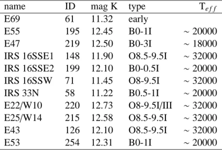
5.2 Stellar types expected in the central parsec . . . . 36

5.3 HB/RC template stars . . . . 37

6.1 Classified stars . . . . 60

6.2 Density power law parameters . . . . 65

6.3 KLF power law parameters . . . . 66

6.4 Early type stars detected outside of 0.5 pc . . . . 69

7.1 Fitting results for polarization parameters (P1,P2) . . . . 81

7.2 Polarization parameters for sources common to Ks/Lp-band . . . . 88

7.3 Polarization parameters for sources common to H/Ks/Lp-band . . . . 89

8.1 Polarization parameters measured for IRS 21 (Ks-band) . . . . 97

Table of Abbreviations

AGB Asymptotic Giant Branch AGN Active Galactic Nucleus

AO Adaptive Optics

CBD CO band depth

CND Circumnuclear Disk

ESO European Southern Observatory FOV Field of View

FWHM Full Width at Half Maximum

GC Galactic Center

HB Horizontal Branch

IB Intermediate Band

IMBH Intermediate Mass Black Hole IMF Initial Mass Function

IRS Infrared Source ISM Interstellar Medium

KLF K-band Luminosity Function LR Lucy-Richardson (deconvolution)

MIR Mid-Infrared

NA Northern Arm (of the minispiral)

NB Narrow Band

NIR Near-Infrared

NSC Nuclear Stellar Cluster PSF Point Spread Function

RC Red Clump

SED Spectral Energy Distribution SFR Star Formation Rate

Sgr A* Sagittarius A*

SMBH Supermassive Black Hole

VLT Very Large Telescope

YSO Young Stellar Object

ZAMS Zero Age Main Sequence

1 Introduction

The center of our own Galaxy, the only Nuclear Cluster so far accessible at this level of detail, has been the subject of a multitude of studies over the past decades, since infrared and radio observations first opened up this region to the eyes of astronomers. Evolving observational ca- pabilities, especially the construction of 8m class telescopes like the VLT in Chile and Keck in Hawaii, aided by the development of Adaptive Optics and new detector techniques, have al- lowed a more and more detailed and precise insight into the ”heart” of the Milky Way. And while a new and even larger telescope generation is on the horizon, there are still large blank spots to be filled, even in this well-observed region. The scope of this thesis encompasses two of these formerly blank spots: large-scale, deep stellar classification and high resolution stellar polarization measurements.

Classification of stars based on spectral features has been done in the GC before, and at much higher spectral resolution than what is presented here. So what is new about the method pre- sented in this work, and what new results can it provide? One crucial weakness of spectroscopic instruments is their small field-of-view. Even with an integral field spectrometer like SINFONI (ESO VLT), covering the innermost 1.5 pc as it was done here requires unrealistic amounts of observation time, if sufficient depth and spatial resolution are to be achieved.

This is the advantage of the method used in this work, intermediate-band photometry: the entire region can be observed simultaneously, at the sacrifice of spectral resolution. But the result is sufficient to separate early and late type stars, and based on this, a population analysis can reveal several new aspects: does the old, supposedly relaxed stellar population indeed follow the as- sumptions for such a population in the vicinity of a Supermassive Black Hole? A so-called cusp has been predicted for the very center, an increase in projected density of the late type stars, but as will be shown below, this is clearly not the case. Another aspect is the still ongoing discussion on star formation in the central region, and how this work can contribute to the constraints that have to be placed on stellar evolution models for the GC. The early type density distribution and luminosity function have been investigated before for the brightest of these sources, but can these findings of a steep power law density distribution and a top-heavy initial-mass-function be confirmed on this much larger sample? Are there any signs of tidal tails left behind by an inspi- raling cluster of young stars formed elsewhere, as some models suggest? Or, if star formation indeed takes place in the innermost region, are there any signs of Young Stellar Objects (YSOs)?

The latter question leads to the second part of this work: measuring the polarization parameters of an unprecedented number of sources in the GC in the H-, Ks-, and Lp-band. Observations like that have been undertaken in the past, but only at much lower resolution. Especially in the H- and Lp-band, the latest observations were obtained 25-30 years ago, with the depth and spatial resolution available at that time (a few arcseconds, at that resolution the IRS 16 complex for instance is seen as a single source). High resolution polarimetric observations in the GC can provide new insight in several areas: the line-of-sight polarization and its relation to the ex- tinction can be investigated, intrinsic polarization of compact sources yields information on the processes in the vicinity of these objects and the properties of the surrounding material. The cen- tral parsec offers several promising targets in all three observed wavelength bands, such as the extended bow-shock sources (most likely mass-losing stars plowing through the local medium), dust streamers in the mini-spiral, and candidates for YSOs. Some of these issues could not be explored in depth in this work due to a lack of suitable data, but in addition to the findings al- ready shown here, interesting targets for follow-up observations can be determined (such as the IRS 13N cluster and several bow-shock sources). In addition, the proven feasibility of Lp-band polarimetry with NACO opens up new possibilities to explore the nature of these sources (while NACO is still operational, but the methods developed here could easily be adapted to a successor instrument).

In the following, § 2 gives a short overview of the Galactic Center and introduces some basic

concepts and processes. § 3 details the data reduction methods that were applied to the observa-

tional data, which are presented in § 4. § 5 explains the photometric, polarimetric and calibration

procedures that were used to achieve the results, which are in turn presented in § 6 (stellar clas-

sification and popualtion analysis), § 7 (stellar polarization), and § 8 (polarization and variability

of extended sources). Finally, conclusions and a summary are contained in § 9.

2 The Galactic Center

2.1 The Nuclear Stellar Cluster

The Galactic center (GC) is located at a distance of ∼ 8.0 kpc (Reid, 1993; Eisenhauer et al., 2005; Groenewegen et al., 2008; Ghez et al., 2008; Gillessen et al., 2009; Fritz et al., 2011) from the sun. This value is adopted throughout this work. At this distance, it is much closer than the next closest galactic nucleus in M31 (with 784 kpc, see Holland et al., 1998). The next AGN is even further away ( ∼ 10 times further out than M31).

The immediate center of the GC contains the densest star cluster in the Galaxy with a ∼ 4.0 × 10

M

supermassive black hole at its dynamical center (Eckart et al., 2002; Sch¨odel et al., 2002, 2003; Ghez et al., 2003, 2008; Gillessen et al., 2009). This cluster shows similar properties as the NSCs found at the dynamical and photometric centers of other galaxies (B ¨oker, 2010; Sch¨odel, 2010c). The projected density distribution of the observed stars in this cluster has been described by a broken power law (break radius R

= 6

.0 ± 1

.0, all values given here are projected radii), with a power-law slope of Γ = 0.19 ± 0.05 within the break radius and Γ = 0.75 ± 0.10 towards the outside of the cluster (Sch¨odel et al., 2007).

Around the central parsec itself, a structure made up of dense and warm molecular gas (10

− 10

cm

, several hundred K) is located in several clumps/clouds/filaments moving on a circu- lar orbit around the center, the circum nuclear disk (CND). This structure stretches from about 1.5 pc to 7 pc from the center. The inner edge is relatively steep. Inside this radius, a cavity of mainly atomic and ionized gas (but almost no molecular gas) can be found. From the inner edge, several streamers of gas and dust seem to be on infalling trajectories towards the center. They are interacting with the winds emanating from the stars in the nuclear star cluster. This so-called

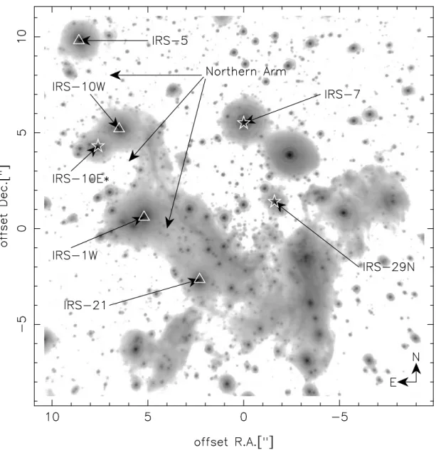
”mini-spiral” (Lacy et al., 1991) appears to consist of a complex threedimensional structure (Paumard et al., 2004) with several sub-components (e.g. the Northern Arm to the north-east of the center). The influence of this structure can be seen on several individual sources (for instance the bow-shock sources in the Northern Arm, see Tanner et al., 2005), as well as in extinction maps of this area (Scoville et al., 2003; Sch¨odel et al., 2010b).

2.1.1 Stellar composition

The stellar composition of the cluster depends on the distance to the center. This has been ob- served first as a drop in CO absorption strength towards Sgr A* in seeing-limited observations (Allen et al., 1990; Sellgren et al., 1990; Haller et al., 1996). Two explanations have been dis- cussed for this: a significantly lower density of late type stars in the central few arcseconds and/or the presence of a large number of bright early type stars. Adaptive optics assisted observations with high spatial resolution have shown that there is indeed an increased number of early-type stars in this region, while the relative number of late type stars decreases (Genzel et al., 2003;

Eisenhauer et al., 2005; Paumard et al., 2006; Lu et al., 2009). Several authors have tried to explain this finding by collisions between stars (or between stellar mass black holes and stars), which may lead to the destruction of the envelopes of giant stars in the central region (Davies et al., 1991; Bailey & Davies, 1999; Rasio & Shapiro, 1990; Davies et al., 1998; Alexander et al., 1999; Dale et al., 2008).

Several stellar populations have been detected in the central parsec: the oldest observable ob-

jects that make up the bulk of the visible sources outside of the innermost few arcseconds are

old, metal-rich M, K and G type giants with ages of 1 − 10 × 10

years. The helium-burning

red clump sources are also present, although they have not been discussed in detail until recently

(Maness et al., 2007), because older works on the stellar population did not reach the necessary

lower magnitude limit. A number of intermediate-bright (mag

∼ 10 − 12) stars that are now on

the AGB (Krabbe et al., 1995; Blum et al., 1996, 2003) have been produced by a star formation

event ≥ 100 × 10

years ago. These stars can be distinguished from late type giants by the H

O

absorption bands in their spectra that are detectable even at low spectral resolution. Very few supergiants like IRS 7 are also present in the central parsec. Several objects with featureless, but very red spectra have also been detected (Becklin et al., 1978; Krabbe et al., 1995; Genzel et al., 1996), namely IRS1W, 3, 9, 10W and 21. With high-resolution imaging, most of these sources have been resolved. They are mostly associated with the mini-spiral, and can be interpreted as young and bright stars with rapid mass loss interacting with the interstellar medium in the GC, so called bowshock sources (Tanner et al. (2002, 2003); Geballe et al. (2004), see also Perger et al. (2008) ). In the central ∼ 0.5 pc there exists yet another distinct stellar population: massive, young stars created in a starburst 3 − 7 × 10

years ago (e.g., Krabbe et al., 1995). These stars can be found, e.g., in the IRS 16 and IRS 13 associations (e.g., Eckart et al., 2004a; Maillard et al., 2004; Lu et al., 2005).The brightest of those young stars have been described as stars in a transitional phase between O supergiants and Wolf-Rayet stars (WN9/Ofpe according to e.g.

Allen et al., 1990), with high mass-loss during this phase (Najarro et al., 1994; Krabbe et al., 1995; Morris et al., 1996; Najarro et al., 1997; Paumard et al., 2001; Moultaka et al., 2005).

These stars account for a large part of the luminosity of the central cluster and also contribute half of the excitation/ionizing luminosity in this region (Rieke, Rieke & Paul , 1989; Najarro et al., 1997; Eckart et al., 1999; Paumard et al., 2006; Martins et al., 2007). Recently, Muzic et al. (2008) have identified a co-moving group of highly reddened stars north of IRS 13 that may be even younger objects, the IRS 13N cluster. These sources are maybe the best candidates for very recent star formation in the central parsec itself, and might therefore provide valuable insight into the star formation mechanism so close to Sgr A*.

Besides the most massive early type stars, a large number of OB stars with masses of ∼ 10-60 M

have been examined by Levin & Beloborodov (2003); Genzel et al. (2003); Paumard et al.

(2006); Lu et al. (2009). At least 50% of the early-type stars in the central 0.5 pc appear to be located within a clockwise (in projection on the sky) rotating disk, which was first detected by Levin & Beloborodov (2003). Later, Genzel et al. (2003); Paumard et al. (2006) claimed the existence of a second, counter-clockwise rotating disk. A very detailed analysis by Lu et al.

(2009), based on the fitting of individual stellar orbits, shows only one disk and a more randomly distributed off-disk population (with the number of stars in the disk similar to that on random orbits). Bartko et al. (2009), however, claim that they at least observe a counter-clockwise struc- ture that could be a strongly warped, possibly dissolving second disk. In the immediate vicinity of Sgr A*, there is yet another distinct group of stars, which form a small cluster of what appear to be early B-type stars (Eckart et al., 1999; Ghez et al., 2003; Eisenhauer et al., 2005). These so-called “S-stars” stars are on closed orbits around Sgr A*, with velocities of up to a few thou- sand km/s and at distances as close as a few lightdays (Sch¨odel et al., 2003; Ghez et al., 2003, 2005; Eisenhauer et al., 2005; Ghez et al., 2008; Gillessen et al., 2009). Their orbits have been used to determine the mass of the black hole and the distance to the GC.

Detailed spectroscopic studies of the stellar population in the central parsec have so far only been conducted in the innermost few arcseconds and on small areas in the outer regions of the cluster (see Ghez et al. (2003, 2008); Eisenhauer et al. (2005); Paumard et al. (2006); Maness et al. (2007)). Here the main limitation is that the high surface density of sources in the GC forces the observers to use high spatial resolution observations in order to be able to examine all but the brightest stars. However, the field-of-view of integral field spectrometers is quite small at the required angular resolutions (e.g., between 3

× 3

and 0.8

× 0.8

for the ESO SINFONI instrument).

2.1.2 Star Formation in the GC?

How exactly star formation can take place in the central parsec under the observed conditions is still a debated issue. Classical star formation from gas of the observed density is severely impeded by the tidal shear exerted by the black hole and the surrounding dense star cluster (Morris et al., 1993). Two scenarios are being discussed to explain the presence of the early type stars: Genzel et al. (2003); Goodman (2003); Levin & Beloborodov (2003); Milosavljevic &

Loeb (2004); Nayakshin & Cuadra (2005); Paumard et al. (2006) suggest a model of in-situ star

formation, where the infall and cooling of a large interstellar cloud could lead to the formation

of a gravitationally unstable disk and the stars would be formed directly out of the fragmenting

disk. An alternative scenario has been proposed by Gerhard (2001); McMillan & Portegies Zwart

(2003); Portegies Zwart et al. (2003); Kim & Morris (2003); Kim et al. (2004); Guerkan & Rasio (2005) with the infalling cluster scenario, where the actual star formation takes place outside of the hostile environment of the central parsec. Bound, massive clusters of young stars can then be transported towards the center within a few Myr (dynamical friction in a massive enough cluster lets it sink in much more rapidly than individual stars, see Gerhard (2001)). Recent data seem to favor continuous, in-situ star-formation (e.g. Nayakshin & Sunyaev (2005); Paumard et al.

(2006); Lu et al. (2009)

The existence of the S stars so close to Sgr A* is yet another matter, known as the ”paradox of youth” (Ghez et al., 2003). Two explanations are discussed for the presence of these stars, though neither is satisfactory: formation out of colliding or interacting giants (Eckart et al., 1993; Genzel et al., 2003; Ghez et al., 2003, 2005) or scattering from the disk of young stars (Alexander & Livio , 2004).

2.2 Extinction

Radiation from distant sources passes through the interstellar medium (ISM) between the source and the observer, and the influence of this medium can be quite significant. Depending on the wavelength, different components of the ISM and different processes become important, such as emission/absorption and scattering on electrons, ions, atoms, molecules and/or dust grains. For broadband near-infrared observations as they were conducted here, the dominant influence that has to be considered is the absorption and scattering of light on dust grains, termed extinction.

Extinction has to main effects on the observations: sources behind a lot of dust appear fainter than expected from their distance and intrinsic brightness. This has to be considered when e.g.

distances are calculated from the apparent brightness of sources of known type:

m

= M

+ 5log(d) − 5 + A

(2.1)

Here, m

and M

denote the apparent respectively absolute magnitude of a source, d is the distance in parsec, and A

is the extinction in magnitudes at a particular wavelength. If the extinction is high enough, the source becomes too faint to be observed any more. This is the case, for instance, with the Galactic Center in the optical, where the extinction reaches 40-50 mag (see below). But the extinction is also wavelength dependent, with much lower values of A

∼ 3 mag towards the GC in the NIR. While this allows observing the GC in these wavelength bands, it leads to another effect: the spectrum of an extincted source is shifted towards the red, since shorter wavelengths suffer higher extinction. The wavelength dependence is complex in general, but in the NIR it can be described by a simple power law (Draine, 1989; Sch¨odel et al., 2010b; Fritz et al., 2011):

A

∝ λ

(2.2)

Draine (1989) proposed β = − 1.75, but recent results by Gosling et al. (2009); Sch¨odel et al.

(2010b); Fritz et al. (2011) suggest a slightly steeper power law with β ∼ 2.0.

2.3 Polarization

In general, three effects can produce polarized NIR radiation in GC sources: (re)emission by heated, non-spherical grains, scattering (on spherical and/or aligned non-spherical grains), and dichroic extinction by aligned dust grains. The first two cases can be, for the purposes of this work, regarded as intrinsic to the source, thereby allowing conclusions about the source itself and its immediate environment, while the third effect is the result of grain alignment averaged along the LOS. For sources enclosed in an optically thick dust shell, dichroic extinction can also contribute significantly as a local effect (see e.g. Whitney & Wolff , 2002).

2.3.1 Foreground polarization

As the basic mechanism that could cause the observed, large scale grain alignment, Davis &

Greenstein (1951) suggested paramagnetic dissipation, which basically aligns the angular mo-

mentum of spinning grains with the magnetic field. But even almost 60 years later, the issue of

grain alignment is by no means completely solved, and it remains difficult to reach exact con- clusions for dust parameters and magnetic field strength, but at least determining the magnetic field orientation is possible. If the parameters change along the LOS, this further complicates the issue. See e.g. Purcell et al. (1971); Lazarian (2003); Lazarian et al. (2007) and references therein for a review of the different possible causes of grain alignment expected to be relevant in different environments.

It is therefore possible to use polarimetric measurements to map at least the direction of the mag- netic fields responsible for dust alignment through the Davis-Greenstein effect, as e.g. Nishiyama et al. (2009, 2010) showed for the innermost 20’ respectively 2

of the GC, but these studies did not cover the central parsec due to insufficient resolution.

Observations of the galactic center suffer from strong extinction caused by dust grains on the LOS, with values of up to A

= 40 mag at optical wavelengths (or even higher values of up to 50 mag if a steeper extinction law is assumed) and still around 3 mag in the Ks-band (e.g.

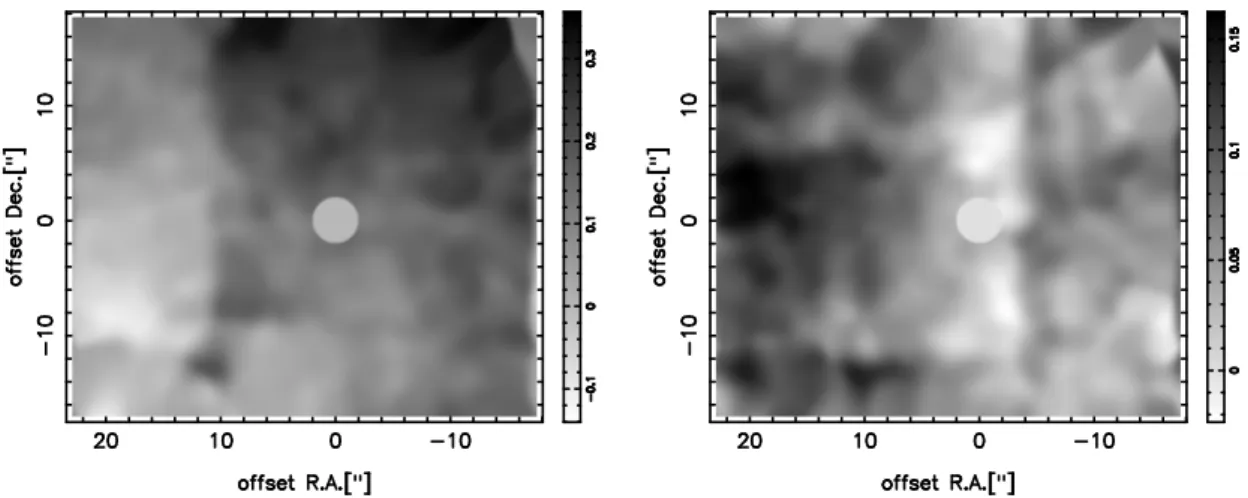
Scoville et al., 2003; Sch¨odel et al., 2010b). The aligned interstellar dust grains responsible for the polarization cause extinction as well, but non-aligned grains can also contribute. Therefore, the same particles are not necessarily responsible for both effects (e.g. Martin et al., 1990). Uni- versal power laws have been claimed for polarization (Martin et al., 1990) (in a similar way as for NIR extinction, see Draine, 1989), who also showed that the law applicable to polarization in the optical domain (Serkowski et al., 1975) is a poor approximation in the NIR. The power law indices presented in these works for the extinction and the polarization power law are almost the same (1.5-2.0). It also appears that there is a correlation between the measured extinction of an intrinsically unpolarized source and foreground polarization (Serkowski et al., 1975), but this relation is quite complex. In the light of new results for the extinction law which seem to deviate consistently from the Draine law (e.g. Gosling et al., 2009; Sch¨odel et al., 2010b), new polarimetric measurements may be useful to further clarify the relation between extinction and polarization. The central parsec of the GC is a well suited but challenging environment to study this relation, since it contains a large number of sources which exhibit large variances in extinction (1-2 mag, see Buchholz et al., 2009; Sch¨odel et al., 2010b), which is produced along a long line-of-sight by a large number of dust clouds with possibly different grain alignment and composition. A new Ks-band extinction map of the central parsec recently been presented by Sch¨odel et al. (2010b) is used as a reference in this work.

2.3.2 Local polarization

In the context of this work, local polarization refers to processes taking place in the innermost region of the GC itself, either around individual sources or in extended local structures such as the arms of the minispiral.Specifically, this encompasses effects of dusty stellar envelopes or disks, the interaction of stellar outflows with the local ISM in bow-shocks, and the emission by heated, aligned grains in dust streamers such as the Northern Arm.

Three basic processes can produce polarization in such environments: emission from elongated and aligned grains, dichroic extinction (also needs grain alignment and elongation), and scat- tering, either in the form of Mie-scattering on spherical grains or scattering on elongated and aligned grains as well. The relative importance of these processes depends on the local dust properties, such as grain size distribution, dust temperature, dust density, magnetic fields, and streaming velocities.

Emission

While a spherical grain would emit radiation isotropically, elongated grains emit preferably along their long axis. If the grain population is aligned, this leads to the radiation being polarized parallel to the mean orientation of the long grain axes. In the case of magnetic alignmment, spinning grains would align their angular momentum with the field (Davis & Greenstein, 1951), so their long axes and thus the polarization are perpendicular to the aligning field.

For a given grain alignment efficiency, the relative importance of polarized emission over the

wavelength bands depends on the size distribution and the temperature of the grains. These two

parameters are related as well, since smaller grains can reach higher temperatures more easily

by absorption of high energy photons or stochastic collisions with high energy electrons or ions

Figure 2.1: Blackbody emission in the H- and Ks-band compared to the Lp-band emission, logarithmic plot. Green dots represent H-band, red dots Ks-band. All fluxes were normalized to the flux in the Lp-band.

(Geballe et al., 2004). Fig.2.1 shows the relation between the emission in the H-, Ks-, and Lp- band at different temperatures. This is only a rough approximation, since the grains are treated as blackbodies here, but it already shows some general trends: for grain temperatures as they are common in the Northern Arm of the minispiral (200-300K, see Smith et al., 1990; Gezari, 1992), emission in the H- and Ks-band is negligible compared to the Lp-band. For higher temperatures of 900-1000K, however, H- and Ks-band emission becomes important as well. Assuming that these trends are essentially the same for the dust grains in the GC, significant emission in the two shorter wavelength bands requires much higher temperatures than what has been observed.

Where such emission is detected, such as around the bright bow-shock sources, the temperatures must be higher due to heating from the central source or in a shock front, and/or scattering must play a significant role.

Local dichroic extinction

As it is the case along the LOS, dichroic extinction can take place locally if the dust column density is high enough. But unlike in the dust clouds along the LOS, where individual sec- tions may show different alignment that cancels out parts of the effect and leaves only a net component of polarization, alignment of local dust can be regarded as uniform on small scales (depending on the local magnetic fields). The local field strength also determines the efficiency of the alignment, and this can also be much higher than what is found in a LOS cloud. In total, the polarization efficiency, i.e. the relation between dust extinction and absorptive polarization, can be far higher than the values found for the foreground polarization: essentially, even a small dust column density can produce dichroic extinction of the same order of magnitude as the fore- ground polarization, if the grains are aligned efficiently.

For a given grain alignment, the polarization produced by this process is perpendicular to the

long axes of the grains (as this is the preferential direction of absorption). Therefore, dichroic

extinction and dust emission from the same grains produce polarization with perpendicular po-

larization angles. If the alignment of the grains is known (e.g. from the magnetic fields and

the streaming motions), and if scattering is not important, the polarization angle can be used to estimate the relative importance of these two processes and thus give an indication of the local dust density.

Scattering

While only non-spherical and aligned grains can produce polarization by emission and dichroic extinction, scattering can take place on spherical grains as well. In this so-called Mie-scattering process, unpolarized light is partly scattered forward on a dust grain (assuming a particle size of the order of magnitude of the wavelength) and partly scattered away perpendicular to its angle of incidence. This latter part is linearly polarized. If a central source is surrounded by an isotropic shell of spherical grains, the scattered light produces a reflection nebula, and this structure shows polarization in a centrosymmetric pattern, with the polarization vectors tangential to concentric circles around the central source. An unresolved source of this kind shows its maximum in polarization if viewed edge-on, while if viewed face-on, it exhibits no linear polarization at all since the contributions from different regions cancel each other out. For a more complicated geometry, such as a dusty disk around a central object as one would expect it in YSOs, the resulting polarization patterns can be more complicated (see e.g. Murakawa, 2010).

Scattering on elongated dust grains is a far less simple problem, and has only recently been modeled: Whitney & Wolff (2002) showed the effects of optical depth, grain geometry and inclination angle on the polarization patterns of dusty disks and spherical structures, using a method developed by Mishchenko et al. (2000) to calculate the scattering properties of non- spherical grains. This study did not cover bow-shock-like structures, however, and while there are theoretical models of bow-shocks (e.g. most recently by Gustafson et al., 2010; van Marle et al., 2011), these do not consider polarization. Therefore, the results obtained in § 8.2 could not be compared directly to theory or models.

2.3.3 Polarization of GC sources

Less than a decade after the first near-infrared (NIR) imaging observations of the Galactic center (GC) by Becklin & Neugebauer (1968), the polarization of 10 sources within ≤ 2 pc of Sagittar- ius A* was measured by Capps & Knacke (1976); Knacke & Capps (1977), observing in the K-, L- and 11.5 µm-band. These observations revealed similar polarization degrees and angles for the 4 sources observed in the K-band, with the polarization angles roughly parallel to the galactic plane ( ∼ 4% at 15

East-of-North, while the projection of the galactic plane is at a position angle of ∼ 31.4

at the location of the GC, see Reid et al., 2004). This was interpreted as polariza- tion induced by aligned dust grains in the Milky Way spiral arms along the line-of-sight (LOS).

The 11.5 µm polarization, however, was found to be almost perpendicular to the galactic plane and was therefore classified as intrinsic. The values found for the L-band showed intermediate values, which was attributed to a superposition of both effects. The GC therefore offers the pos- sibility to study both interstellar polarization as well as the properties of intrinsically polarized sources.

Kobayashi et al. (1980) conducted a survey of K-band polarization in a much wider field of view (7’ × 7’), finding largely uniform polarization along the galactic plane. Lebofsky et al. (1982) confirmed these findings in the H- and K-band for 17 sources in the central cluster. The latest H-band survey was conducted by Bailey et al. (1984), who examined ∼ 10 sources with a 4.5”

resolution, finding similar results. While these surveys could only resolve a small number of sources in the central region, higher resolution observations (0.25”) enabled Eckart et al. (1995) to measure the polarization of 160 sources in the central 13” × 13”, while Ott et al. (1999) exam- ined ∼ 40 bright sources in the central 20” × 20” at 0.5” resolution. These two studies confirmed the known largely uniform foreground polarization, but already revealed a more complex pic- ture: individual sources showed different polarization parameters, such as a significantly higher polarization degree (IRS 21).

These results already illustrated that in addition to the foreground polarization, intrinsic polariza-

tion plays a role in the Ks-band as well, and not only at longer wavelengths. Especially sources

embedded in the Northern Arm and other bow-shock sources (see Fig.4.2 for an overview of the

bright bow-shock sources in the central 20”) show signs of intrinsic polarization. Among these

objects, IRS 21 shows the strongest total Ks-band polarization of a bright GC source detected to

date ( ∼ 10-16% at 16

Eckart et al., 1995; Ott et al., 1999). Tanner et al. (2002) described IRS 21

as a bow-shock most likely created by a mass-losing Wolf-Rayet star. The observed polarization

is a superposition of foreground polarization and source intrinsic polarization. It is still unclear

what process(es) cause the latter component: (Mie)-scattering in the dusty environment of the

Northern Arm and/or emission from magnetically aligned dust. The latter is known to occur at

12.5 µm (Aitken et al., 1998), but should be negligible at shorter wavelengths.

3 Data reduction techniques

3.1 Cleaning the Image

3.1.1 Standard procedure

The NAOS/CONICA-instrument produces 1024 by 1024 pixel images, using an InSb Aladdin 3 detector. The nature of the detector chip itself and the wavelength regime (NIR-MIR) create several problems that have to be dealt with before the actual photometry can commence. For this task, the dpuser software

provides a number of algorithms.

• Dead/hot pixels on the chip: it needs to be avoided that pixels that either do not respond at all (dead) or always register a very high number of counts (hot) pollute the data (e.g. by mistaking a collection of hot pixels for an actual source). These pixels are detected and their values replaced by an average over the neighboring pixels.

• Flat-fielding: during the photometry, it is assumed that every region of the detector reg- isters a given photon flux as the same number of counts. This is not the case with any real detector, however, since the production process and aging lead to inhomogeneities.

To counter this, the detector is illuminated by an artificial light source, and several images are taken with the lamp switched on/off (lamp-flat method). The on and off images are then subtracted, averaged, and the actual data are divided by these flat-fields, in order to achieve the same calibrated detector response for the whole image.

• Sky subtraction: flux from emission in the atmosphere itself is a major issue with NIR and MIR observations, and this influence becomes stronger at longer wavelenghts: in the Lp-band, the sky emission exceeds the flux of all but the brightest sources in the GC.

This can be compensated by taking images of source-free areas not too far from the main target, and then subtracting these sky exposures from the on-source images. In the H- and Ks-band, taking sky measurements only once or a small number of times during the night is sufficient (depending on observing conditions, a more variable sky necessitates more frequent sky measurements). For Lp-band observations, even small variations of the large sky contribution become important, so a sky exposure is taken after every image of the target.

3.1.2 Pattern removal

Even after the sky-subtraction and flat-fielding, the March 2011 Lp-band images still contained significant patterns. These are not actual structures in the Galactic center itself (as a comparison with previous Lp-band observations reveals, see e.g. Viehmann et al., 2005), but must have been introduced either by the detector itself or possibly by the sky correction. This can happen when the sky exposures contain sources themselves. Due to the high sky flux, these cannot be easily made out and masked, as it can be done in the Ks- or H-band. Two distinct patterns occur in all images: a series of ’stripes’ along the East-West-axis and a ’cloudy’ structure in the east and west of the FOV. The latter occurs at the same position in each image, while the former is different for each exposure.

The East-West pattern was approximated by averaging over the x-axis of each image (excluding bright pixels, in order to avoid a bias from the stars). The resulting profile was subtracted from the image. This does not introduce a significant bias, since there are no large scale East-West structures expected in this FOV.

In order to remove the stationary pattern, an average image was computed from all individual exposures (excluding the stellar sources) for each polarization channel. This yielded a charac- teristic pattern for each channel, which was then subtracted from all images.

1

written by T. Ott, the software is available at http://www.mpe.mpg.de/ ∼ ott/dpuser/

Before and after the removal of each pattern, each image was shifted to a background level centered around zero. This turned out to be necessary since the background level after sky sub- traction varied on the order of 10-20 counts between individual images. With a highly variable sky (due to less-than-optimal observing conditions), this can be expected: the flux from the sky alone reaches 2000-3000 counts per pixel, so a change of 1% between sky and object exposure already produces an offset of 20-30 counts. Unfortunately, this means that the background flux cannot be measured and any information about the background polarization is lost.

3.2 Deconvolution

Even in the optimal case that the influence of the atmosphere can be neglected, the image of a point source produced with any optical system suffers degradations because of the limitations of the instrument. In the ideal case of an aberration-free telescope with a circular aperture, the image of a point source would basically be an Airy pattern. When the effects of the atmosphere and the imperfections of the telescope are added to this, the result is a specific point spread function (PSF). This function is variable with time, due to temporal variations in the instrument itself and turbulence in the atmosphere (which in turn limits the coherence time), and it also varies over the FOV (anisoplanasy).

Thus, the observed signal g(x, y) can be described as a convolution of the observed object f (x, y) with a function describing the PSF, h(x, y), and another function describing other influences like the detector read-out noise, anisoplanasy and other non-linear terms, c(x, y):

g(x, y) = f (x, y) ⊙ h(x, y) + c(x, y) (3.1) with ⊙ denoting the convolution operator.

Technical improvements like Adaptive Optics and the construction of larger telescopes on the ground and in space are a way to minimize these effects, but some PSF residuals will always remain. The basic idea of deconvolution is therefore to replace the complicated PSF with some- thing that allows easier accurate photometry and also improves the detectability of faint sources, such as a Gaussian PSF with a FWHM of the order of the diffraction limit.

A convolution like this corresponds to a multiplication in Fourier space. Therefore, in pricin- ple, the Fourier transform of the original object could be (in the ideal case without noise and non-linear effects) determined by a simple divison in Fourier space (F(u, v), G(u, v), H(u, v) denoting the Fourier transforms of f (x, y), g(x, y), h(x, y), with u, v as the spatial frequencies corresponding to the coordinates x and y):

F(u, v) = G(u, v)

H(u, v) (3.2)

What has to be considered, however, is that any telescope has a limited aperture, which in turn means that H(u, v) will be zero at very high frequencies, and thus information on high spatial frequencies is lost. Also, the image degradation term c(x, y) (non-linear effects, noise) cannot be neglected in any real case, and especially the noise can become dominant at high spatial frequen- cies. The PSF also cannot be determined with perfect accuracy, as it is usually approximated or extracted from several sources in the image. Therefore, this simple approach does not work, so several methods have been devised to find at least the most probable object distribution. In this work, the Linear Deconvolution algorithm and the Lucy-Richardson Deconvolution method are used.

3.3 Linear Deconvolution

The linear deconvolution method basically adapts the discussed Fourier division to deal with the issues of an issufficiently determined PSF and noise. For this purpose, a so-called Wiener filter (designated Ψ in the following) for the suppression of high spatial frequencies is introduced.

The reconstruction of the object can then be described in Fourier space by the following:

O(u, v) = [G(u, v) + C(u, v)] × Ψ(u, v)

H(u, v) (3.3)

The filter then has to be chosen so that the difference between this expression and F(u, v) (the

’real’ object) is minimized:

Z

−∞

[(G(u, v) + C(u, v)] × Ψ(u, v)

H(u, v) − G(u, v) H(u, v)

2

d(u, v) = Minimum (3.4) Deriving this expression with respect to Ψ and setting the result equal to zero leads to

Ψ(u, v) = | G(u, v) |

| G(u, v) |

+ | C(u, v) |

(3.5) It has to be considered that the signal and the noise are uncorrelated, so

Z

−∞

(G(u, v) × C(u, v))d(u, v) = 0. (3.6)

The spectral energy distribution of the signal can be approximated by that of the observed PSF ( | G(u, v) |

≈ | H(u, v) |

), while the noise spectral energy distribution is reasonably well repre- sented by a delta function ( | δ(u, v) |

). If one takes into account that the power spectrum of a function is given by the product of its fourier transform and the complex conjugate of the fourier transform ( | H(u, v) |

= H(u, v) × H(u, v)), this finally yields (neglecting the noise term in equation 3.3)

F(u, v) ≈ O(u, v) ≈ G(u, v) × H(u, v)

| H(u, v) |

+ | δ(u, v) |

(3.7)

3.4 Lucy-Richardson Deconvolution

The Lucy-Richardson (LR) deconvolution algorithm is an iterative process based on the scheme for the rectification of observed probability distributions proposed by Lucy (1974). This scheme consists of the iteration of three steps. First, the current estimate of the object distribution O

(x, y) is convolved with the PSF estimate H(x, y):

L

(x, y) = O

(x, y) ⊙ H(x, y) (3.8) The image obtained this way, L

(x, y), is compared with the observed image G(x, y):

R(x, y) = G(x, y)

L

(x, y) ⊙ H(x, y) (3.9)

with the PSF acting as a low-pass filter reducing the influence of high frequencies on the re- sult because those are affected much stronger by noise. Finally, a new estimate of the object distribution is obtained by multiplying the original estimate with the correction function R(x, y):

O

(x, y) = O

(x, y) ⊙ R(x, y) (3.10) The convolution with the PSF suppresses high spatial frequencies, thus avoiding the amplifi- cation of noise peaks. But also, any details of the image related to high spatial frequencies, like close binary stars, can only be observed after a high number of iterations ( ∼ 10

). This already points out one big disadvantage of this method, the high amount of computation time that is required. Especially if a large number of images has to be processed, or the same image has to be processed a large number of times like for a completeness correction, this method is slow compared to others (such as Linear Deconvolution). Another disadvantage is the fact that very faint sources and diffuse emission close to bright sources tend to be added to the flux of the bright source. This effect can be observed as a negative residuum around bright sources.

The only way to minimize this is a very precise determination of the PSF including its faint

wings. Furthermore, the diffuse background of the image tends to be resolved into distinct point

sources. These can be excluded by comparing different images, as it is done when creating the

common list anyway (see § 5.1.1).

4 Observations

4.1 General parameters

All observations used here were carried out with the NAOS-CONICA (NACO) instrument at the ESO VLT unit telescope (UT) 4 on Paranal. The bright super-giant IRS 7 located about 6” north of Sgr A* was used to close the feedback loop of the adaptive optics (AO) system, thus making use of the infrared wavefront sensor installed with NAOS. For the H- and Ks-band observations (including intermediate band data), the sky background was determined by taking several dithered exposures of a region largely devoid of stars, a dark cloud 713” west and 400”

north of Sgr A*. In the Lp-band, alternating sky and object exposures were taken using a region 60” west and 60” north of Sgr A* to determine a largely source-free sky.

All images were flat-fielded, sky subtracted and corrected for dead/hot pixels.

In order to determine the quality of individual observations, the Strehl ratio was adopted as a criterion. This parameter describes the ratio of the flux contained in the core of the measured point-spread-function (PSF) in the image to that expected for a theoretical PSF calculated from telescope parameters (for a given wavelength). The Strehl ratio was determined using the strehl algorithm in the ESO eclipse software package

.

4.2 Intermediate band data

The data used for the stellar classification were taken in June/July 2004 and April 2006 (pro- grams 073.B-0084(A), 073.B-0745(A), 077.B-0014(A), see Tab.4.1 for details, datasets N1-N7 and H18), using an H band broadband filter and seven intermediate band filters. The seeing var- ied for the different observations, within a range of 0.5 to 1.3”. A rectangular dither pattern was used for most observations, while some were randomly dithered. This led to a total field-of-view (FOV) of 40.5”, corresponding to ∼ 1.5 pc.

In order to be able to separate early and late type sources using the CO band depth method de- scribed in § 5.1.6, the photometry has to be accurate enough to clearly identify the feature used for the classification (see § 5.1.3). This means that the typical photometric error should be much lower than the typical depth of the classification feature (see § 5.1.3 for an estimate of the re- quired accuracy). When observing a large field of view like in this case, a good AO correction can only be achieved within the isoplanatic patch, typically a region of ∼ 10-15” for the available data. This effect leads to a decrease of the Strehl ratio towards the outer regions of the field (see Fig.5.1). This value was computed from the PSFs determined in 12 × 12 subimages of the IB227 image (with the same PSF stars that were used in the photometry). The Strehl values exhibit a clear trend towards lower values at larger projected distances from the guide star. Sources out- side of the isoplanatic patch show a characteristic elongation towards IRS 7. This is a problem when using PSF fitting photometry, while aperture photometry (which is less dependent on the shape of the PSF) is faced with the problem of crowding.

4.3 Polarimetric data

The main polarimetric datasets used in this work were obtained in June 2004 (H-band broad- band filter, program 073.B-0084A, dataset P1, see Tab.4.1), May 2009 (Ks-band broadband filter, program 083.B-0031A, dataset P2) and March 2011 (Ks- and Lp-band filters, program 086.C-0049A, datasets P16 and P18. In addition, several polarimetric Ks-band datasets con- tained in the ESO archive (datasets P3-P15)

were used, in order to expand the total FOV and

1

see N. Devillard, ”The eclipse software”, The messenger No 87 - March 1997, publicly available at http://www.eso.org/projects/aot/eclipse/distrib/index.html

2

Based on observations collected at the European Organization for Astronomical Research in the Southern Hemi-

sphere, Chile