Variable Source Sagittarius A*
INAUGURAL-DISSERTATION
zur
Erlangung des Doktorgrades
der Mathematisch-Naturwissenschaftlichen Fakult¨at der Universit¨at zu K¨oln
vorgelegt von
Gunther Witzel aus Bonn
K¨oln 2012
Prof. Dr. Peter Schneider
Tag der m¨undlichen Pr¨ufung: 04. 04. 2012
Zusammenfassung V
Abstract VII
1. Introduction 1
1.1. Adaptive optics measurements . . . . 3
1.2. The variable near-infrared source Sgr A* . . . . 6
1.3. Radiation mechanisms . . . . 8
2. A statistical analysis of the variability of Sgr A* in the near-infrared 13 2.0.1. Definitions and concepts . . . . 13
2.0.2. NIR time series of SgrA* . . . . 15
2.1. Data reduction . . . . 17
2.1.1. The data base . . . . 17
2.1.2. Data reduction and flux density calibration . . . . 17
2.1.3. Light curves of Sgr A* . . . . 21
2.2. Statistical analysis of the flux density distribution . . . . 23
2.2.1. Optimal data visualization . . . . 23
2.2.2. Power-law representation of the intrinsic flux density distribution 27 2.3. Time series analysis . . . . 36
2.3.1. RMS-flux density relation . . . . 37
2.3.2. Simulating light curves . . . . 38
2.3.3. The structure function and the PSD . . . . 42
2.4. Extreme flux density excursions and the X-ray echo . . . . 51
2.4.1. Maximum expected NIR flux density . . . . 51
2.4.2. A possible explanation of the X-ray light echo . . . . 52
2.5. Summary . . . . 54
3. Near Infrared Polarimetry 57 3.1. Basics of Polarimetry . . . . 58
3.2. Metallic reflection . . . . 60
3.3. The optical train of NACO . . . . 61
3.4. A model for the instrumental polarization of NACO . . . . 62
3.4.1. Instrumental polarization generated by M3 . . . . 62
3.4.2. The IP of the adaptive optics module NAOS . . . . 64
3.4.3. The retarder plate . . . . 64
3.4.4. The entire instrumental polarization of NACO . . . . 66
3.5. The instrumental polarization in numbers . . . . 66
3.6. CONICA and the polarimetric analyzer . . . . 68
3.6.1. M¨uller-matrix for transmittance differences . . . . 70
3.6.2. Flat-field correction . . . . 71
3.7. Correcting the data for the instrumental systematics . . . . 74
3.8. Observations . . . . 75
3.8.1. The data . . . . 75
3.8.2. Gauging the model: standards and IRS16 stars . . . . 77
3.9. Comparison of different calibration methods . . . . 80
3.9.1. The “channel switch” method . . . . 80
3.9.2. The “boot strapping” method . . . . 82
3.9.3. Effects on time-resolved polarimetric measurements of Sgr A* 85 3.10. Summary . . . . 85
4. Conclusions and perspectives 87
A. Data quality 89
B. Light curves 91
C. Flux density statistics 107
D. Correction matrices for the optical components of NACO 109 E. Supplement information for the polarimetric calibration of NACO 113
Abbreviations 117
Bibliography 119
List of Figures 130
List of Tables 131
Danksagung 133
Im Focus dieser Dissertation steht die hochvariable Strahlungsquelle im Zentrum un- serer Milchstraße Sagittarius A* (Sgr A*). Die Arbeit umfasst zwei Teile: eine um- fassende Darstellung der vorhandenen Ks-band (Nahinfrarot-) Beobachtungen mit dem Very Large Telescope der Europ¨aischen S¨udsternwarte aus den letzten sieben Jahren und eine Analyse der instrumentellen systematischen Effekte bei polarimetrischen Mes- sungen mit der adaptiven Optik NAOS und der Kamera CONICA.
Im ersten Teil charakterisiere ich die statistischen Eigenschaften der Nahinfrarotvari- abilit¨at von Sgr A*, einer Quelle, die in direktem Zusammenhang mit dem zentralen Schwarzen Loch im Zentrum unserer Milchstraße gesehen wird. Ich zeige, dass zur Beschreibung der Flussdichteverteilung ein einfaches Potenzgesetz geeignet ist. Somit kann die an anderer Stelle ge¨außerte Ansicht, dass die Flussdichteverteilung einen klaren Bruch und somit einen Hinweis auf zwei verschiedene Variabilit¨atsprozesse gibt, nicht best¨atigt werden. Ich weise eine lineare Abh¨angigkeit der Variabilit¨at von der Flussdichtehelligkeit der Quelle nach. Dieser Befund zusammen mit der Potenz- gesetzverteilung impliziert ein ph¨anomenologisches, formal nicht-lineares statistisches Variabilit¨atsmodell, mit dem es mir gelungen ist, Lichtkurven zu simulieren, deren Charakteristika und zeitliches Verhalten den beobachteten entsprechen, und die Vorher- sagen f¨ur - im Beobachtungszeitraum nicht nachgewiesene - h¨ohere Flußdichten und lange Zeitskalen zulassen. Mit diesem Modell l¨asst sich zeigen, dass ein Helligkeits- ausbruch, wie er m¨oglicherweise in den letzten 400 Jahren stattgefunden hat - wof¨ur ein Lichtecho im R¨ontgenbereich emittiert von Molek¨ulwolken in der weiten Umge- bung von Sgr A* spricht - durchaus als Extremwert der gefundenen Statistik erkl¨arbar ist. Weiterhin kann ich zeigen, dass Aussagen dar¨uber, inwieweit ausgezeichnete Zeit- skalen k¨urzer als 100 min bei dem zeitlichen Verhalten der Variabilit¨at wesentlich sind, mit den hier pr¨asentierten Daten nicht gemacht werden k¨onnen. Dies ist eine Frage, die im Zusammenhang mit orbitalen Bewegungen in der Akkretionscheibe des Schwarzen Loches nahe am Ereignishorizont diskutiert wird.
Im zweiten Teil analysiere ich die instrumentelle Polarisation von NAOS/CONICA, einer Nahinfrarotkamera mit adaptiver Optik. Ziel war es, den Einfluss dieser syste- matischen Effekte auf Zeitreihen der polarimetrischen Parameter im Falle von Sgr A*
zu bestimmen. Hierzu habe ich den Stokes/M¨uller-Formalismus zur Beschreibung der
Effekte metallischer Reflektion auf den Polarisationszustand herangezogen. Das so be-
stimmte Modell der instrumentellen Polarisation wurde mit Beobachtungen von Kali- brationsquellen verglichen. Desweiteren habe ich verschiedene ¨ubliche Kalibrations- methoden in ihrer Wirkung anhand von Simulationen und anhand dreier ausgew¨ahlter Lichkurven verglichen. Als Ergebnis habe ich eine deutliche Abh¨angigkeit der instru- mentellen, maximal 4-prozentigen Polarisation von der Ausrichtung des Telekops und außerdem eine fehlerhafte Eichung der Vorzugsrichtung der Verz¨ogerungspl¨attchens nachgewiesen. Mit dem neuen Modell der instrumentellen Polarisation wird es m¨oglich sein, Genauigkeiten von etwa einem Prozentpunkt im Polarisationsgrad und, im Falle von Quellen mit Polarisationsgraden h¨oher als 4%, 5 ◦ Winkelgenauigkeit zu ereichen.
F¨ur Zeitreihenmessungen wie im Falle von Sgr A* ¨uberwiegen die statistischen Fehler.
This thesis on observational astronomy focuses on the highly variable near-infrared source Sagittarius A* (Sgr A*) at the center of the Milky Way, associated with the central 4 × 10 6 M super-massive black hole. It is divided in two parts: a compre- hensive data description of Ks-band measurements of Sgr A*, covering the last seven years of observations with the Very Large Telescope and the state-of-the-art instrument NAOS/CONICA, and an effort in polarimetric instrumentation, the calibration of the instrumental polarization properties of NAOS/CONICA in the Ks-band.
In the first part I characterize the statistical properties of the near-infrared variability of Sgr A*, the electromagnetic manifestation of the Galactic Center super-massive black hole, and find the flux density to be power-law distributed. I cannot confirm the evidence of a two state process with different flux density distributions behind the variability, as reported in other publications. I find a linear rms-flux relation for the flux density range up to 12 mJy on a timescale of 24 minutes. This and the power- law flux density distribution imply a phenomenological, formally non-linear statistical variability model with which I can simulate the observed variability and extrapolate its behavior to higher flux levels and longer timescales. I can show that a bright outburst within the last 400 years, that has been discussed as the possible reason for the X- ray emission from massive molecular clouds surrounding the Galactic Center, can be expected as an extreme value of our statistics without the need for a cosmic event.
I give arguments, why data with our time support cannot be used to decide on the question whether the power spectral density of the underlying random process shows more structure at timescales below 100 min compared to what is expected from a red noise random process, as discussed in the context of orbiting hot spots in the accretion flow of the black hole.
In the second part I report on the results of calibrating and simulating the instrumen-
tal polarization properties of the Very Large Telescope adaptive optics camera system
NAOS/CONICA (NACO) in the Ks-band. Here my goal was to understand the influ-
ence of systematic calibration effects on the time-resolved polarimetric observations
of Sgr A*. I used the Stokes/Mueller formalism for metallic reflections to describe the
instrumental polarization. The model is compared to standard-star observations and
time-resolved observations of bright sources in the Galactic Center. I simulated the
differences between calibration methods and tested their influence on three examples
of polarimetric Ks-band light curves of Sgr A*. I find the instrumental polarization to
be highly dependent on the pointing position of the telescope and about 4% at max-
imum. I report a polarization angle offset of 13.2 ◦ due to a position angle offset of
the λ /2-wave plate with respect to the data-header value that affects the calibration of
NACO data taken before autumn 2009. With the new model of the instrumental polar-
ization of NACO it is possible to measure the polarization with an accuracy of 1% in
polarization degree. The uncertainty of the polarization angle is ≤ 5 ◦ for polarization
degrees ≥ 4%. For densely sampled polarimetric time series I find that the improved
understanding of the polarization properties gives results that are consistent with the
previously used method to derive the polarization of Sgr A*. The difference between
the derived and the previously employed polarization calibration is well within the sta-
tistical uncertainties of the measurements, and for Sgr A* they do not affect the results
from our relativistic modeling of the accretion process.
image: NASA, ESA, and Q.D. Wang (University of Massachusetts, Amherst). Credit for Chandra image: NASA/CXC/UMass/D. Wang et al.
1. Introduction
The existence of galaxies is a discovery of the early twentieth century. Edwin Hub-
ble found the Andromeda nebula to be far more distant than the objects in the Milky
Way, and opened the door to extragalactic astronomy. Since then the development
of new and powerful telescopes and principles, covering the whole electromagnetic
spectrum, while reaching an astonishing resolution and sensitivity, has empowered as-
tronomers to make unprecedented progress in discovering exotic objects and decipher-
ing the physical processes in the near and far distant universe. Although seemingly
trivial, an important step was the identification of our own Milky Way as a barred
spiral galaxy. As a matter of fact, objects in our Milky Way allow the most detailed
studies due to their proximity. A key method of astronomical research is to compare
and complement our knowledge about the structure and the physical processes in our
Milky Way with what we know about other, more distant galaxies and vice versa. The distance of extragalactic objects has another aspect: because of the finite speed of light we are not only looking in to the far distance, but also into the past. Due to this fact we can infer information on the evolution of galaxies that happens on time scales no human life span or cultural deliverance could cover otherwise.
In the last decades a class of very exotic objects, first discovered as very luminous sources (the so called Quasars), started playing a central role: black holes. It is a widely accepted fact that all or at least most of the galaxies house a super-massive (millions and billions of solar masses) black hole at their center. The correlation of the masses with other properties of the housing galaxies implies a connection between the evolution of the super-massive black holes and the galaxies. The discovery of the radio source Sagittarius A* by Balick & Brown (1974) and the subsequent supply of evidence for a compact object with 4 × 10 6 solar masses in the center of our galaxy showed that our Milky Way is no exception in this respect. This makes the center of the Milky Way a unique opportunity to study processes associated with black holes and their interaction with the hosting galaxies in detail.
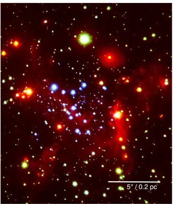
5'' / 0.2 pc
Fig. 1.2.: HKL-composite of the nuclear cluster.
The dynamical center of our galaxy is at a distance of about 8 kpc (e.g. Sch¨odel et al.
2002). The innermost parsecs are a very dynamical region that contains a dense nu-
clear star cluster, dense molecular clouds, supernova remnants, a dense molecular ring
orbiting the nucleus on a scale of a few parsecs, and a three arm structure of ion- ized gas, the so called mini-spiral. This variety of structures and objects only can be investigated by combining observations at different wavelengths. Fig. 1.1 gives an im- pression, how different the innermost 240 × 120 light-years look like in the infrared, near-infrared and X-ray regime. At optical wavelengths the line of sight towards the very center is obscured by dust, resulting in an extinction of a factor of 10 −12 . The multi-wavelength approach is necessary not only to reveal different constituents of the central region, but also different aspects of the radiation processes of the individual objects. The most particular object is situated at the heart of the nuclear star cluster:
the radio, near-infrared and X-ray source Sagittarius A* (Sgr A*) that is the electro- magnetic manifestation of the central black hole of our galaxy. The evidence that this object indeed can be associated with a super-massive black hole was established in essence by two important findings: the very little proper motion of the compact source itself, determined from VLBI radio measurements (Backer & Sramek 1999; Reid et al.
1999), and the precise determination of the orbits of in the meantime about 30 stars within the S-star cluster in the near-infrared (NIR), resulting in an estimation of the enclosed mass of about 4.4 × 10 6 solar masses (Eckart & Genzel 1996, 1997; Eckart et al. 2002; Sch¨odel et al. 2002; Eisenhauer et al. 2003; Ghez et al. 2000, 2005, 2008;
Gillessen et al. 2009). Fig. 1.2 shows a three color composite of NIR observations in the H-, Ks- and L-band of the innermost parsec around Sgr A*.
1.1. Adaptive optics measurements
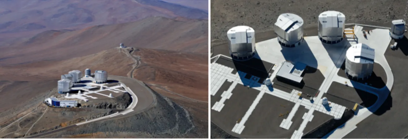
Numerous measurements of the stellar orbits, and the observations this thesis is based on, have been conducted with one of the most advanced telescopes of our time, the Very Large Telescope (VLT) of the European Southern Observatory (ESO) in the north of Chile. This observatory, located at 2600 m over sea level on Paranal mountain in the middle of the Atacama desert, runs four telescopes with 8.2 m mirrors, each supported by an active optics system and equipped with optical and infrared instruments, and four smaller auxiliary telescopes.
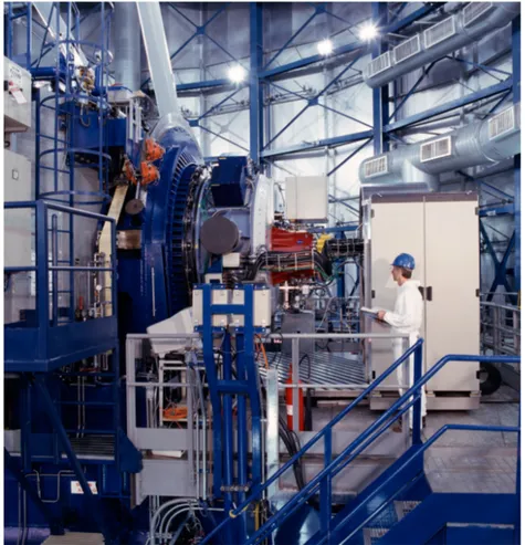
The NIR instrument with which the astrometric measurements mentioned before and the database of this thesis have been obtained is NAOS/CONICA (NACO), mounted at one of the Nasmyth foci of the Unit Telescope 4 (Yepun). This instrument provides adaptive optics corrected observations in the wavelength range of 1− 5 µ m 1 . It consists of the adaptive optics system NAOS and the imager and spectrograph CONICA which includes a mode for differential polarimetric imaging.
1
For the technical descriptions of the VLT and the AO system I follow Eckart et al. (2005), Bertram
(2007) and Ageorges et al. (2007).
Fig. 1.3.: The Very Large Telescope observatory in the Atacama dessert in the north of Chile. Image courtesy:ESO/H¨udepohl (atacamaphoto.com)
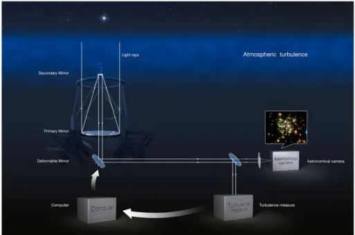
Atmospheric turbulence on the line-of-sight causes fluctuations of the refractive index on a wide range of spatial and temporal scales. These fluctuations distort the otherwise flat wavefronts of light coming from far distant astronomical objects and hence do not allow a better resolution than about 0.7 arcsec in the NIR. For high angular resolution ground based imaging adaptive optics overcome this restriction and nearly reach a resolution at the diffraction limit.
Single aperture adaptive optics (AO) is a real time system for measuring phase pertur- bations of the wavefront by a phase reference source and correcting them in a closed loop. It enables the observer to obtain images at the diffraction limit with long integra- tion times. The phase reference source has to be located within the so called isoplanatic patch around the target where the atmospheric transfer function is almost constant. The low frequency perturbations are usually corrected by an additional system, a so called tip-tilt sensor and correcting mirror. This system corrects for the displacement of the image on the detector. The higher frequency contributions are corrected with the higher order AO system that restores the wavefront with a deformable mirror (DM) that is lo- cated close to a pupil image of the conjugated atmospheric layer where the turbulence occurs. The DM has a size of 10 to 20 cm and is equipped with an arrangement of piezoelectric actuators (a few hundred for 8 m-class telescopes in NIR) that shape the mirror into a conjugate of the measured aberrations. The corrections have to be done on time scales of a few 10 to 100 Hz and with an accuracy of λ /20 to λ /50. The seeing and thus the requirements of an AO system depend on the wavelength. In NIR the isoplanatic patch is in the oder of 20 00 . In the visible domain it can drop down to about 5 00 . Common AO systems correct at wavelengths longer than 1 µ m.
Fig. 1.5 shows a schematic view of a typical AO loop. For determining the distor-
tions different devices are used: Shack-Hartmann, pyramid wavefront, and curvature
sensors. The Shack-Hartmann device that is used in the case of NAOS divides the tele-
Fig. 1.4.: NAOS/CONICA at the Nasmyth focus of VLT UT 4, Yepun. The red cylinder is the camera system CONICA. Image courtesy:ESO.
scope pupil into multiple sub-pupils. Several images of the point-like reference source occur on the detector and the slope of the wavefront at the position of the sub-pupil can be measured from the displacement of the sub-images with respect to a reference posi- tion. The control loop between the wavefront sensor and the deformable mirror has to be very fast. The necessary commands have to be calculated within about 1 millisec- ond. In order to minimize the integration times a bright star (brighter than magnitude 17 in the visible and magnitude 10 in the NIR domain) is required. The necessity of the presence of bright stars reduces the sky coverage to a few percent. To overcome this problem artificial laser guide stars are used.
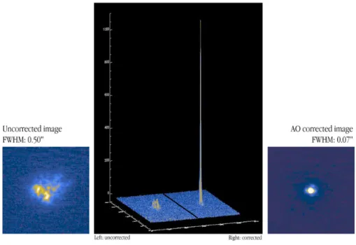
The corrected PSF typically contains a diffraction limited core and a broad seeing foot
that has a similar or even larger size than the uncorrected seeing cloud.This is essential
for the discussion of halo noise below (see section 2.2.2). A measure of the quality
of the correction is the so called Strehl ratio, the ratio between the peak intensity of
the corrected and the peak intensity of the theoretical point spread function (PSF). A
demonstration of the improvement of the Strehl ratio by adaptive optics is shown in
fig. 1.6.
Fig. 1.5.: Scheme of an adaptive optics system. Image courtesy:ESO.
A comprehensive overview on Galactic Center research is given in Genzel et al. (2010), Eckart et al. (2005) and Melia (2007). A description of the physical mechanisms in- volved in imaging through the atmosphere and their mathematical treatment can be found in Bertram (2007) and references therein.
1.2. The variable near-infrared source Sgr A*
Sgr A*, located at the center of the our galaxy, is a highly variable near-infrared and X-ray source. While first detected as a bright, ultra compact, and comparatively steady radio source, the strong variability in the NIR and X-ray regime, and the variable polar- ization of the NIR emission provide reasonable ground to believe that properties of the black hole and its emission and accretion mechanisms can be studied at these wave- lengths (Baganoff et al. 2001; Porquet et al. 2003, 2008; Genzel et al. 2003; Eckart et al. 2004, 2006a,c,b, 2008a,b,c; Yusef-Zadeh et al. 2006a,b, 2007, 2008; Dodds-Eden et al. 2009; Sabha et al. 2010).
Since the first near-infrared (NIR) polarimetric Wollaston prism observation of Sgr A*
in 2004 (Eckart et al. 2006a), polarized flares have been regularly observed (Meyer
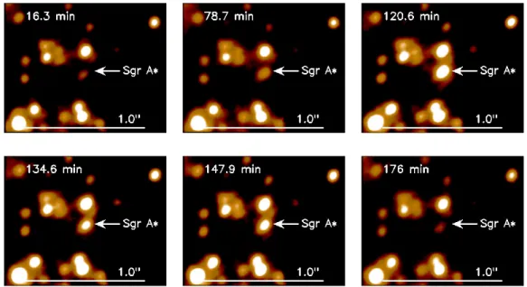
et al. 2006a,b, 2007; Eckart et al. 2008a, Zamaninasab et al. 2010). In the NIR short
bursts of increased emission exceeding 5 mJy occur four to six times a day and last
typically for about 100 minutes (see Fig. 1.7). The linear polarization degrees can
reach 20% to 50% of the total intensity. The polarized NIR flares are often associated
with simultaneous X-ray flares (Baganoff et al. 2001; Porquet et al. 2003, 2008; Gen-
zel et al. 2003; Eckart et al. 2004, 2006a,c,b, 2008a,b,c; Meyer et al. 2006a,b, 2007;
Fig. 1.6.: Improvement of the Strehl ratio by the AO system of NACO. Image courtesy:ESO.
Yusef-Zadeh et al. 2006a,b, 2007, 2008; Dodds-Eden et al. 2009; Sabha et al. 2010), suggesting Synchrotron Self-Compton (SSC) or inverse Compton emission as the re- sponsible radiation mechanisms (Eckart et al. 2004, 2006a,c; Yuan et al. 2004; Liu et al. 2006; Eckart et al. 2012).
Considering the time behavior of the polarized NIR light curves some models that as- sume the variability to be linked to emission from single or multiple hot spots in the accretion disk near the last stable orbit of the black hole have been applied success- fully to individual datasets (Meyer et al. 2006a,b, 2007; Zamaninasab et al. 2008). But within the discussion about the role of timescales and, in particular, the presence of a quasi-periodic oscillation (QPO) corresponding to orbital motion near the innermost stable orbit of the black hole, Do et al. (2009) argue that QPOs in total intensity light curves cannot be established with sufficient significance against random fluctuations.
On the other hand, based on relativistic models, Zamaninasab et al. (2010) predicted a correlation between the modulations of the observed flux density light curves and changes in polarimetric data (also see Eckart et al. 2006a, Meyer et al. 2006a, Meyer et al. 2006b, Meyer et al. 2007; Eckart et al. 2008a, Cunningham & Bardeen 1973;
Stark & Connors 1977; Abramowicz et al. 1991; Karas & Bao 1992; Hollywood et al.
1995; Dovˇciak et al. 2004, Dovˇciak et al. 2008). A comparison of predicted and ob-
served light curve features (obtained from 7 nights of polarimetric observations with
VLT and Subaru telescope) through a pattern recognition algorithm resulted in the de-
tection of a signature possibly associated with orbiting matter under the influence of
strong gravity. This pattern is found to be statistically significant against randomly
Fig. 1.7.: Sgr A* in a flaring state. These pictures show NIR K-band measurements from 2007.
polarized red noise.
1.3. Radiation mechanisms
Sgr A* is very under-luminous with respect to its Eddington limit (10 −8.5 L Edd , Genzel et al. 2010). The Eddington luminosity is the maximum luminosity for a symmetrical accretion flow and is reached in the case of equilibrium between the inward driving gravitational force and the outward driving radiative force originating from the inner part of the accretion flow. This made it necessary to develop the so called radiatively inefficient accretion flow models.
Sgr A* shows a combination of time invariant and variable emission at all wave- lengths 2 . While in the NIR and X-ray domain Sgr A* is highly variable, the emis- sion in the radio domain is comparatively quiescent. As summarized in Genzel et al.
(2010) this can be explained by a steady state emitting predominantly at radio and sub- millimeter wavelength originating from synchrotron emission of a thermal distribution of relativistic electrons, and a variable state generated by transiently heated electrons.
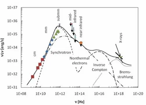
In Fig. 1.8 I show the steady state spectral energy distribution (SED) of Sgr A* that, for the different parts of the spectrum, can be modeled by synchrotron emission from thermal and non-thermal relativistic electrons, inverse Compton up-scattering of the synchrotron photons by thermal electrons, and by a Bremsstrahlung contribution. It is important to note that the quiescent state SED at mid- to near-infrared wavelength
2
In the description of the steady radiation mechanisms I follow Genzel et al. (2010).
is not well determined because the quiescent fluxes at these frequencies are below the detection limits. Because of the limited sensitivity and resolution of the instruments in addition to the extended structures visible at these wavelengths only upper limits could be obtained.
Fig. 1.8.: Steady state spectral energy distribution of Sgr A* from Genzel et al. (2010) and references therein. At the radio frequencies it is well described by synchrotron emission from thermal relativistic electrons (dashed line) with a flattening toward lower frequencies due to a con- tribution from non-thermal electrons (dashed-dotted line). The long dashed line represents a contribution of inverse Compton up-scattering of synchrotron photons by thermal electrons, the steady emission in the X-ray domain is dominated by Bremsstrahlung from the outer part of the accretion flow (dotted line).
The processes behind the variable part are still under debate. While many ideas and models are linked, as mentioned before, to accretion mechanism within an accretion disc, there are also approaches involving the foot point of a short jet (Falcke & Markoff 2000; Yuan et al. 2003; Markoff et al. 2001; Markoff & Falcke 2003). In Eckart et al.
(2012) we show that a very likely explanation for the synchronous NIR and X-ray out-
bursts are synchrotron and synchrotron self-Compton mechanisms. In this model that
is able to reproduce the behavior of all cases of observed simultaneous NIR and X-
ray variability a synchrotron spectrum with a turnover frequency from optically thick
to optically thin emission at a few hundred GHz to one THz is dominating the NIR
emission. The X-ray flares are linked to this NIR-variability by inverse Compoton-
scattering of the synchrotron photons by the same population of relativistic electrons
that are generating the synchrotron radiation. Another important radiation mechanism
is connected to correlations between the NIR and sub-mm variability, as they are re-
ported in Eckart et al. (2008c). Flares in the sub-mm occur with delays of 0.75 to 2 hours with respect to the NIR, and adiabatic expansion describes the evolving flux densities of both wavelength very well. The expansion speed for these emitting regions are of the order of 0.005 c and very low compared to the expected relativistic sound speed in orbital velocity in the vicinity of the super-massive black hole, resulting in ei- ther a large bulk motion of the adiabatically expanding source components or a strong confinement within the immediate surrounding of Sgr A*.
In the case of the relativistic modeling of the polarimetric Ks-band fluctuations in Za- maninasab et al. (2008) and Zamaninasab et al. (2010) the appearance of a possibly evolving hot spot for an observer far from the black hole under relativistic effects like boosting and lensing, and in particular the expected development of the polarization degree and angle, lead to a typical pattern of the polarimetric parameters, as mentioned above. This pattern basically includes a distinct total intensity peak, with a preceding rapid change in polarization angle (a common feature of many strong gravity scenar- ios) and a following peak in polarization degree. From an observer’s point of view it is unfortunate that a strong depolarization attends the rapid change of the angle, be- cause for a reliable determination of the polarization angle significant polarized flux is essential, and calibration problems or instrumental effects can easily generate similar patterns, as it is discussed in chapter 3.5.
In Genzel et al. (2010) the authors point out that “in the interpretation of the observed variability it is a key issue whether the brightest variable emission from Sgr A* at near-infrared and X-ray wavelength are statistical fluctuations from the probability dis- tribution at low flux, or flare events with distinct properties”. Indeed, the interpretation of a two state variability process with bright flares on top of moderate fluctuations seems to be suggested by the X-ray light curves that exhibit very bright distinct peaks.
The authors speculate that the contrasting subsumption of the short timescale variabil- ity (on the one hand as an orbital signature in the accretion flow (e.g. Genzel et al.
2003; Eckart et al. 2006c; Dodds-Eden et al. 2009), and on the other hand as purely statistical fluctuations originating from featureless red noise (Do et al. 2009) can be explained by the transition between both variability states. They suggest a bright, po- larized, power-law flux distributed flaring state with significant detection of QPOs, and a fainter, log-normal distributed stochastic process. This interpretation is based on the findings by Dodds-Eden et al. (2011), as described in detail in chapter 2.
The motivation for the work presented in this thesis is to investigate the robustness
of the proposed double state scenario. It considers two aspects: the statistics of the
Ks-band NIR variability, and the robustness of the calibration of the polarimetric ob-
servations. The key question mentioned above is answered in the next chapter as far as
it is possible on the base of the available data.
In chapter 2 I present the results of my investigation of Ks-band flux density time
series of Sgr A*. In chapter 3 I describe my analysis of the polarimetric mode of
NAOS/CONICA. In chapter 4 I present conclusions and perspectives for future steps
in analyzing the variability of Sgr A*. In the Appendix supplement information is
presented.
variability of Sgr A* in the near-infrared
2.0.1. Definitions and concepts
First, I want to introduce some mathematical concepts which the following analysis is based on. This serves as a short recapitulation of some important definitions. I follow the definitions and notation of Priestley (1982) and Theiler et al. (1993).
A random process is defined as a sequence of random variables X(t), with t, in our case, a discrete sequence of time points. A time series is a sequence of measurements x(t ) which can be considered as a particular realization of the underlying random process.
The probabilistic behavior is fully described if we are given the joint probability of {X (t 1 ), X(t 2 ), X (t 3 ), ...,X (t n )} for all n and all choices for t 1 , t 2 , t 3 , ..., t n . Under the assumption of weak stationarity (stationarity up to order m = 2), the mean, variance and the autocorrelation function become time invariant and contain all information about the main characteristics of the time behavior. A random process is stationary up to order m = 2 if, for any t 1 , t 2 ,t 3 , ...,t n and k, all joint moments up to order m = 2 of {X (t 1 ), X(t 2 ), X (t 3 ), ..., X(t n )} exist and equal the corresponding joint moments up to order m = 2 of {X(t 1 + k), X(t 2 + k), X (t 3 + k), ..., X (t n + k)}. A stationary process is also ergodic, i.e. the mean, the variance, and the autocorrelation function can be obtained from the values at different time points of a single realization and do not require the availability of many realizations.
The autocorrelation function is defined as:
ρ(τ) = h[X (t) − µ ][X (t + τ) − µ ]i
σ 2 , (2.1)
with σ 2 the variance of the (stationary) random process and τ a time separation. The autocorrelation function quantifies, so to say, the memory of the random process, i.e.
given a value at a time t it describes the time interval on which probabilistic predictions
can be made with a certain accuracy. Another approach to describe the time behavior
is the power spectral density (PSD), which, under general conditions of existence and
stationarity, is defined for zero mean processes as the Fourier transform of the autocor-
relation function. The PSD describes the time behavior in terms of the average (over all realizations) of the contribution to the total “power” from components in X (t) with a given frequency. A PSD has the properties of a probability distribution and, in par- ticular, is normalized to the total power realized in the process. Statistical estimators of the PSD are called periodograms (see e.g. Priestley 1982).
The coherence timescale (or correlation timescale) of a process can be understood as the time separation of two points where the autocorrelation function falls below a certain value sufficiently close to zero and remains below this limit for larger τ, i.e. it represents the typical timescale where the process loses its memory.
As we will see in this chapter, light curves with a time correlation that is described by a power-law distributed PSD are of special interest. If the power-law slope is larger than unity such a correlation often is referred to as ”red noise”. In the case of red noise light curves the correlation timescale corresponds to the frequency where the power- law describing the PSD breaks (and, e.g., forms a constant plateau). If the length of the observation is shorter than the correlation timescale the observed time series is called weakly non-stationary.
The PSD might show several timescales where the characteristic of the correlation changes, e.g. represented by changes of the slope of the power-law. These distinct timescales do not represent the memory of the total process, but are also referred to as correlation timescales (this looser definition is plausible in the case of, e.g., a sum of independent processes with different correlation timescales).
An important tool to access information on the time behavior of a stationary process is the structure function. The first order structure function for a finite data sequence is defined in section 2.3.3. As Simonetti et al. (1985) show, the structure function is proportional to τ 2 , where τ is a time separation much shorter than the shortest correla- tion time of the random process, and constant for τ greater than the longest correlation time scale. As we will see later, for non-equally spaced data the interpretation of the structure function becomes more challenging.
A stationary linear random process (discrete and equally sampled) is defined as:
X k =
∞
∑
i=0
g i ε k−i , (2.2)
with X k the kth data point, {ε t } being a purely random process (uncorrelated for all k)
and {g i } a sequence of constants satisfying ∑ ∞ i=0 g 2 i < ∞. If X k for each k is Gaussian
distributed, it is called a Gaussian linear random process. Finite discrete parts of a re-
alization of a Gaussian linear random process can be obtained for any PSD by drawing
Fourier coefficients (for each frequency) from a zero mean Gaussian distribution with
width σ proportional to the PSD value, and subsequent Fourier transformation to the
time domain (Timmer & Koenig 1995).
Since the first detection of variable emission of Sgr A* in the NIR in 2003 (Genzel et al.
2003), apart from Zamaninasab et al. (2010) a number of publications concentrated on the statistical properties of the flaring activity rather than on interpreting individual observations. Based on NIR light curves of 7 nights observed with Keck telescope Do et al. (2009) analyzed the flux distribution of Sgr A* and the significance of quasi peri- odic oscillations, finding a pure red noise behavior. They conclude that during fainter states of Sgr A* at maximum 35% of the flux arising at the position of Sgr A* is of stellar origin, attributing the major part to a continuously variable process associated with the black hole. On the base of 14 light curves observed between 2004 and 2008, including very long alternating observations with VLT and Keck, Meyer et al. (2009) discovered first a dominant timescale at about 150 min, supporting linear scaling rela- tions of break timescales of the PSD with the black hole mass. They determined the power-law slope of the high frequency part of the PSD to be 2.1 ± 0.5. A wide multi- wavelength study was conducted by Yusef-Zadeh et al. (2009), including 7 half days of Hubble space telescope data and 6 nights of VLT data, observed alternating in NIR wave-length regime. The authors analyzed the flux density histograms and modeled typical light curves by a sum of Gaussian profiles. Bremer et al. (2011) investigated the H-Ks-band spectral index 1 for bright phases of Sgr A* based on an unprecedent- edly large database covering about seven years of NIR VLT data, and found a spectral index of α = −0.7 as can be expected for pure synchrotron radiation. An analysis by Eckart et al. (2012) of 8 simultaneous X-ray and NIR flares in combination with multi-wavelength observations in 2009 shows that a robust description of all multi- wavelength flare events only can be reached under the assumption of a synchrotron - synchrotron self-Compton radiation mechanism.
The up to now most comprehensive statistical approach in the analysis of the Ks-band total intensity variability observed with NACO at the VLT has been conducted by Dodds-Eden et al. (2011). In this analysis the authors give an overview about the difficult confusion situation in the crowded field around Sgr A* that makes an analysis of the faint emission difficult. They also emphasize the importance of these faint states for the overall statistical evaluation of the variability of Sgr A*. The authors analyzed all VLT K-band data between 2004 and 2009, resulting in a detailed investigation of the flux density statistics. Based on the flux density histogram the authors claim the evidence for two states of variability, a log-normal distributed quiescent state for fluxes
< 5 mJy, and a power-law distributed flaring state for fluxes > 5 mJy, arguing that it seems to be very unlikely that the same variability process is responsible for both high
1
The spectral index is a measure of the dependence of the flux density on the observational frequency.
For the flux density S and the frequency ν it is defined as α (ν) =
dlog[S(ν)]dlog[ν]
.
and low flux emission from Sgr A*. As a description for the observed distribution of the flux density x (measured in mJy) Dodds-Eden et al. (2011) suggest the following probability density:
P 0+err (x) = Z
P 0 (x 0 ) 1
√ 2π σ obs (x) exp
−(x − x 0 ) 2 2σ obs (x) 2
dx 0 (2.3)
i.e., a convolution of an Gaussian error with flux density-dependent width σ obs
mJy = 0.174 · x
mJy 0.5
(2.4) and an intrinsic two state probability density:
P 0 (x) =
( kP logn (x) : x ≤ x b + x t kP logn (x t + x b ) x−x
b
x
t−s
: x > x t + x b (2.5) with k a dimensionless normalizing factor, and the log-normal part defined as
P logn (x) = 1
√ 2π σ ∗ (x − x b ) exp
− h
ln x−x
b
mJy
− µ ∗ i 2
2σ ∗ 2
(2.6)
The parameters of their best fit model are σ ∗ = 0.75, µ ∗ = 0.05, s = 2.7, x t = 4.6 mJy, and x b = 3.59 mJy (here the unit of the probability density is mJy −1 ).
My statistical analysis presented in this thesis serves the following goals:
• to provide a more comprehensive, uniformly reduced data set of Ks-band obser- vations from 2003 to early 2010;
• to conduct a rigorous analysis of the observed flux density distribution;
• to explain why a proper statistical analysis of the Ks-band light curves cannot reproduce the results found by Dodds-Eden et al. (2011);
• to conduct a rigorous time series analysis on the base of a representative dataset;
• to propose a comprehensive statistical model that, using standard methods for generating Fourier transform based surrogate data, describes all aspects of the observed (total intensity) data and allows to simulate light curves with the ob- served time behavior and flux density distribution;
• and to investigate extreme variability events in the context of my statistics.
2.1. Data reduction
In the following I describe the data and the reduction methods I applied in order to ob- tain time-resolved photometric information on Sgr A*. Whereas the data base in large portions is the same as used for the analysis by Dodds-Eden et al. (2011), I have cho- sen different reduction methods: Lucy-Richardson deconvolution in order to guarantee the best possible isolation of the target sources from nearby point-like sources and to minimize the contribution of extended flux, a well controlled flux density calibration with 13 stars, and an objective quality cut based upon seeing and Strehl ratio values.
2.1.1. The data base
My analysis is based on ESO archive data. All observations have been conducted with the NIR adaptive optics instrument NAOS/CONICA at the Very Large Telescope (VLT) in Chile (Lenzen et al. 2003; Rousset et al. 2003). I included all available Ks- band frames of the central cluster of the GC from early 2003 to mid of 2010. For all observations the NIR wavefront sensor of the NAOS adaptive optics system was used to lock on the NIR bright supergiant IRS 7 (variable, m Ks = 6.5 in the 1990s, m Ks = 7.4 in 2006 and m Ks = 7.7 in 2011, 5.6 00 north of Sgr A*). Two different cameras, S13 and S27, with 13 00 and 27 00 field of view 2 , respectively, and a polarimetric mode with inserted Wollaston prism and mask have been available. The latter restricted the area of calibrators that are in common for all frames, to the innermost arcsecond around Sgr A*.
I concentrated on datasets with a length of more than 40 minutes (shorter datasets are often severely affected by bad weather conditions in which case the observer decided fast to change to another wavelength or target). Problematic sets or frames, which showed particular behavior during the basic reduction steps or do not show Sgr A* or a sufficient number of calibrators, have not been included for the photometric analysis.
Ultimately I investigated 12855 frames photometrically. Table B.1 shows a list of all datasets that are part of this analysis. Two restrictions for timing analysis are obvious:
Sgr A* is observed best in the second half of the night in the winter of the southern hemisphere. At other times Sgr A* is located below or close to the horizon or not observable at all due to daylight.
2.1.2. Data reduction and flux density calibration
I performed every reduction step for every frame as uniformly as possible. The reduc- tion included basic steps like a careful sky subtraction and flat fielding, and correction
2
and accordingly with different pixel sampling
for bad pixels. For total intensity data I used a sky flat field if available, for polarimetric data a lamp flat field (Witzel et al. 2011). Most of the data was observed using a jitter routine with random offsets to prevent systematical influences on the measurements by detector artifacts. These offsets need to be detected and corrected for to guaran- tee stable aperture photometry at a constant position. This was achieved with a cross correlation algorithm for sub-pixel accuracy alignment (ESO Eclipse Jitter, Devillard 1999). For each aligned frame I determined an estimate of the point spread function (PSF) with the IDL routine Starfinder (Diolaiti et al. 2000) using isolated stars in the 2 00 surrounding of Sgr A*. The PSF-fitting algorithm of Starfinder provided an estimate of the extended background in each single frame and a list of detected stars with position and relative flux density. I decided not to use the values resulting from Starfinder pho- tometry (for a detailed reasoning see below). Instead I used the Lucy-Richardson (LR) deconvolution algorithm to separate neighboring point-like sources. In order to reduce the contribution of artificial point-like sources that the LR algorithm randomly creates from extended flux I subtracted half the average over the background frame obtained by Starfinder as a constant value from each image. This significantly reduces the white noise contribution to the photometric measurement. In the case of polarization data I aligned all (four to six) polarization channels of each observation night with the cross correlation algorithm, and in the case of data observed with the different pixel scale of the S27 camera (0.02715 00 ) I resampled the pixel scale to 0.01327 00 (S13). Finally a beam restoration was carried out with a Gaussian beam of a FWHM corresponding to the resolution at 2.2µ m (∼ 60 mas).
S27 S26
S6
S35
S30
S8
S10
S98 S100
S84 S7
S65
S107 B
S17 C1
SGRA*
C2
S32 S33 S21 S43 S12
1''
Fig. 2.1.: Ks-band image from 2004 September 30. The red circles mark the constant stars (Rafelski et al. 2007) which have been used as calibrators, the blue the position of photometric mea- surements of Sgr A*, comparison stars and comparison apertures for background estimation.
Source identifications from Gillessen et al. (2009).
After the described preparative steps I conducted aperture photometry with 8 back-
star m Ks flux density [mJy]
S26 14.94 6.79
S27 15.41 4.41
S6 15.35 4.66
S7 14.92 6.92
S8 14.21 13.31
S35 13.20 33.74
S10 13.95 16.91
S65 13.58 23.78
S30 14.12 14.46
S98 15.27 5.01
S100 15.29 4.92
S84 14.66 8.79
S107 14.82 7.59
Table 2.1.: This table shows a list of my calibrators. The flux density for each star was calculated correcting for extinction with m
ext= 2.46.
ground apertures and at the position of 13 constant calibrators (Rafelski et al. 2007), of 6 comparison stars, and at the position of Sgr A* (see Fig. 2.1). The background was estimated at the location of lowest background (6 apertures) and close to Sgr A*
(2 apertures) where no obvious point-like source is visible. I applied a circular mask- ing of radius 0.04 00 at the measurement positions. For a small number of observations, according to the available field of view, I accepted a smaller set of calibrators (at least seven).
The positions of the apertures in each night have been defined as consistently as possi- ble: For Sgr A* with the help of its brighter states, for the stars with the help of mosaics (averages over the single frames of one night in order to increase the signal to noise and to also estimate the centroid of the fainter comparison stars) carefully following their proper motions. For the background apertures and the aperture of Sgr A* when it was faint I conducted triangulation relative to nearby stars. One set of positions then was used for all frames of the corresponding night. For some polarimetric observa- tions NACO was rotated. In these cases I determined a rotation matrix for the position coordinates, making them comparable to the closest unrotated observations.
For each aperture I summed up its total content in analog-to-digital units (ADU). For the polarimetric data the obtained ADU values of orthogonal channels were added.
I subtracted the average background value (B-apertures) in ADU from the calibrator
values and conducted a flux density calibration using the photometric values for the
calibrators in Tab. 2.1.2 (R. Sch¨odel, priv. communication). Because of the high
proper motions of the stars within this field the state of confusion of the calibrators
changes from epoch to epoch. I applied the following algorithm to reduce the epoch- dependent systematic error of the calibration:
First I calculated for each calibrator k the quantity:
f k
ADU = c k
ADU · 10 0.4·m
ref, (2.7)
with c k the background subtracted ADU values for the k-th calibrator, and m ref its reference magnitude. I sorted these values, rejected the three largest and the three smallest values (for the data sets with less calibrators I accordingly reject a smaller number), and took the arithmetic average f 0 over the remaining values. With the zero point from Tokunaga (2000) I then obtained the magnitude m A and flux density F A for each aperture A by
m A = −2.5 · log c k
f 0
F A = 667 · 10 3 · 10 −0.4·(m
A−m
ext) , (2.8) with m ext = 2.46 the K-band extinction correction as determined in Sch¨odel et al.
(2010). This procedure ensures a best possible constance of the flux density calibration under the changing conditions of each dataset.
As a last step I collected parameters for each frame that provide information on the data and calibration quality and allowed me to reject data points based on objective criteria.
These parameters are: Julian date, integration time (NDITxDIT), rotator position angle (orientation of NACO), airmass, guide star seeing, coherence time of the atmosphere, camera, all obtained from the header of the fits data, and the number of stars detected by Starfinder, the Strehl ratio calculated from the extracted PSF using the ESO Eclipse routine STREHL, the average deviation of the calibrators from their literature value, the RMS of the values f k , and, as the most important quality check, the average flux of the calibrators. This last quantity is obtained for each frame by dividing the single measured flux density by the reference value and averaging over all available (i.e. not rejected) calibrators.
I emphasize that both methods - PSF-fitting and Lucy-Richardson aperture photometry
- for estimating the flux density of a point source are in general equivalently well work-
ing as Meyer et al. (2008) have shown. On the other hand, in the case of the presence of
extended flux underlying a (in comparison to the background) dim and confused point
source observed under varying correction performance of the AO-system, the fitting
statistics (i.e. the way Starfinder divides the given flux at a position into background
and point source flux, the over-estimation of the flux due to noise-peaks if the center
of the fit is not fixed, and the statistics of non-detections due to the quality thresholds
set in Starfinder) are difficult to control for this big data set with inhomogeneous cor- rection conditions. I have to mention that also deconvolution has drawbacks, namely a lower astrometric accuracy I have to account for with a suitable big aperture. But the statistics of the interplay between the background (coming from non-resolved sources, truly extended emission and PSF contributions from the surrounding point sources), AO and point-like flux at a given position is directly propagated to the statistics of the measured fluxes, which is crucial for understanding the instrumental influence on my flux statistics. Especially my statistics do not suffer from non-detections that might introduce a selection effect. I will come back to the measurement statistics in section 2.2.
2.1.3. Light curves of Sgr A*
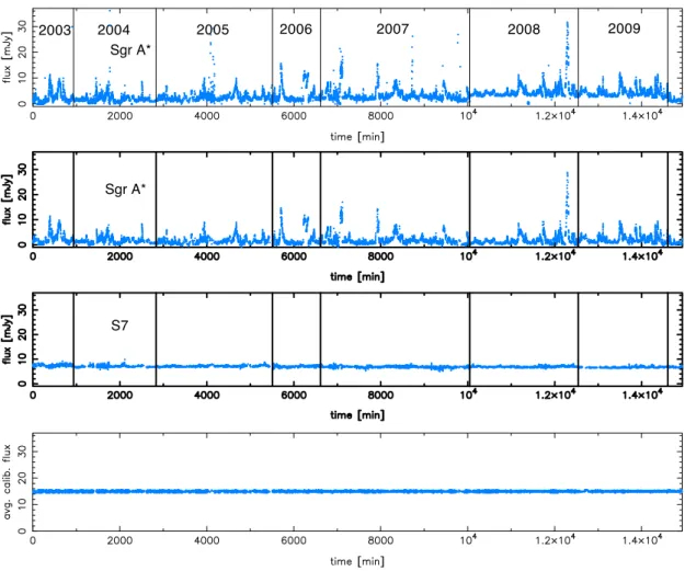
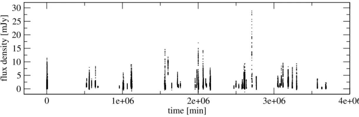
As a result of the reduction procedure described in section 2.1.2 I obtained the data shown in the upper panel of Fig. 2.2. For convenience and following the visualiza- tion used in Dodds-Eden et al. (2011) I show a concatenated light curve with all time gaps longer than 30 minutes removed. This visualization shows the data of all nights as a pseudo-continuous light curve allowing for a comparison of the variability and the confusion in each epoch. A visualization of the true time support is presented in Fig. 2.3. The timing analysis in section 2.3 is based on the true time support, and not on the concatenated light curve.
These 12855 data points still include points of bad observation conditions and insuf- ficient calibration reliability. I used an objective frame rejection algorithm by incor- porating information on seeing (only frames with seeing < 2 00 accepted), Strehl ratio (only frames > 6%), fraction of stars detected by Starfinder 3 , the standard deviation of the f 0 -values (obtained from the individual calibrators for each frame) normalized by the average f 0 -value (only frames < 16%), and the normalized average calibrator flux density as described in section 2.1.2 (only frames > 0.96 and < 1.04).
The top panel of Fig. 2.2 additionally shows a long-time trend of the data from year to year. With respect to these “offsets” of the lowest measured flux densities between the years I follow the analysis by Dodds-Eden et al. (2011) and their conclusion that confusion by faint stars is responsible for this long-time trend. In order to make the different years comparable I subtracted the median of the lowest 5% of each epoch, resulting in 0 mJy for 2003, 0.3 mJy for 2004, 1.0 mJy for 2005, 1.0 mJy for 2006, 1.3 mJy for 2007, 2.8 mJy for 2008, 2.1 mJy for 2009, and 0.7 mJy for 2010. The strong
3
This is a method to reject frames of worse quality than the majority of the individual observation
night. For each sub-frame of the night (i.e. the part of the jittered frames that is common to all)
I count the stars detected by Starfinder. I then calculate the average number of detections over the
night and the standard deviation and reject all frames with a negative deviation from the average of
more than 1.7 times the standard deviation.
2003 2004 2005 2006 2007 2008 2009 Sgr A*
Sgr A*
S7
Fig. 2.2.: The concatenated light curve of Sgr A* and S7, time gaps longer than 30 minutes removed.
The top panel shows the result of aperture photometry before the quality cut, the next panel
the same data after quality cut. The third shows a light curve of S 7, a nearby star that has
been used as a calibrator. The time gaps are the result of the rejection procedure described
in section 2.1.2. The lower panel shows the average ratio between the measured flux of each
calibrator and its reference value (Tab. 2.1.2), scaled with a factor of 15. Its noise corresponds
to the error a hypothetical noise-free aperture with a flux density of 15 mJy would have only
due to the uncertainties of the calibrators.
0 1e+06 2e+06 3e+06 4e+06 time [min]
0 5 10 15 20 25 30
flux density [mJy]
Fig. 2.3.: Light curve of Sgr A* like in Fig. 2.2. In this case no time gaps have been removed, the data is shown in its true time coverage. A comparison of both plots shows: only about 0.4% of the 7 years have been covered by observations.
confusion by the star S2 in 2003 and 2004 4 could be suppressed by the deconvolution reduction step.
The second panel of Fig. 2.2 shows the data after quality cut and subtraction of the faint stellar contribution. For comparison and as an indicator of the calibration stability I show additionally the light curve of one of the calibrators, S7, in the third panel, and in the lowest the average calibrator flux density scaled to 15 mJy.
For a more detailed inspection I present 112 data blocks (defined by continuity, not interrupted by gaps longer than 30 minutes) in Appendix B.
2.2. Statistical analysis of the flux density distribution
In this section I investigate the properties of the flux density statistics of the variability of Sgr A*. This analysis gives information on both the intrinsic flux density distribu- tion of the variability as well as the instrumental effects within our measurements. The differentiation between instrumental features within the distribution and the intrinsic component turns out to be crucial in the context of the question whether the intrinsic flux density distribution provides evidence for two physical mechanisms at work. Ad- ditionally, this analysis allows me to develop a full statistical model of the variability of Sgr A* in the next section.
2.2.1. Optimal data visualization
The first step in the analysis of the flux density distribution of Sgr A* is a proper graph- ical representation of the data in form of a histogram. Histograms are non-parametric
4
which is the reason why Dodds-Eden et al. (2011) did not include the 2003 data and which is clearly
visible in the 2004 epoch of their uncorrected light curve
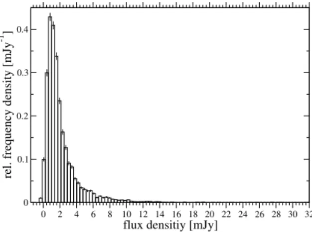
estimators for the probability density behind the sample. A representation of my data in a simple flux density histogram, normalized by total number of points and bin size, is shown in Fig. 2.4.
0 2 4 6 8 10 12 14 16 18 20 22 24 26 28 30 32
flux densitiy [mJy]
0 0.1 0.2 0.3 0.4
rel. frequency density [mJy-1 ]
Fig. 2.4.: Flux density histogram of Sgr A*, based on the data shown in Fig. 2.2
To investigate the high flux density tail of this distribution a logarithmic histogram with an equally spaced logarithmic binning is best suited. The number of bins for a given data range is a crucial parameter for the evaluation of the structure of the sample distribution. Following the study of Knuth (2006) I first determine the best bin size.
As the author points out, the idea is to choose a number of bins sufficiently large to capture the major features in the data while ignoring fine details due to random sampling fluctuations. By considering the histogram as a piecewise-constant model of the probability density function from which n data points x i were sampled the author derives an expression for the relative logarithmic posterior probability (RLP) for each bin number:
RLP = n logN + N log Γ N
2
+ log Γ 1
2
− log Γ
n + N 2
+
N
∑
λ =1
log Γ
n λ + 1 2
. (2.9)
with N the number of bins and n λ the value of the λ th bin. To find the best number of bins M the posterior probability has to be maximized:
M = arg max
N {RLP} . (2.10)
The best estimator for the bin value µ λ and its variance σ λ 2 given the bin values n λ is
deduced to be:
µ λ = M
v
n λ + 1 2 n + M 2
!
(2.11) and
σ λ 2 = M
v 2 "
n λ + 1 2
n − n λ + M−1 2 n + M 2 + 1
n + M 2 2
#
. (2.12)
with v the interval between the maximum and the minimum measurement value.
Knuth (2006) demonstrates in his study that these results outperform several other rules for choosing bin sizes, e.g. “Scott’s rule” or “Stone’s rule”.
I applied the described binning method to my data of Sgr A*. To make the flux density distribution comparable to the results by Dodds-Eden et al. (2011), which include the flux density of the star S17 due to a double aperture method, I added 3 mJy to the flux density of Sgr A*. I find a best bin number of M = 32. The dependence of the log posterior on the bin number is shown in Fig. 2.5. The best piecewise-constant model describing my sample is shown in Fig. 2.6 Unless stated otherwise the histograms in this thesis have been created using this method.
10 20 30 40 50 60 70 80 90 100
number of bins
3300 3350 3400 3450 3500 3550 3600
rel. log. Posterior Probability
Fig. 2.5.: Optimal data based binning. I show the log posterior probability as a function of the number of bins. The maximum for the logarithmic flux density of Sgr A* is reached for 32 bins.
Additionally to the best histogram model obtained from Eq. (2.11) and Eq. (2.12) I over-plotted a graph of the distribution 5 proposed by Dodds-Eden et al. (2011) . It is obvious that my sample is more populated in the middle flux density range between 5 mJy and 15 mJy and shows a linear behavior between 4 mJy and 17 mJy, not showing any break or change of slope. That the shape of my histogram is not sensitive to the binning is shown in Appendix C, Fig. C.1, where I present histograms with 22 bins for the range of the observed flux density values (resulting in a comparable bin width
5
slightly shifted on the x-axis to account for the proper offset due to the double aperture method used
by Dodds-Eden et al. (2011), which before I included only roughly by adding 3 mJy, and to make it
fit best the extremes of my histogram
2 4 8 16 32
flux density [mJy]
1e-05 0.0001 0.001 0.01 0.1 1
rel. frequency density [mJy-1 ]
Fig. 2.6.: Best piecewise-constant probability density model for the flux densities of Sgr A*. The red er- ror bars are the uncertainty of the bin height for the full amount of 10639 data points. The sec- ond bin height visible in some cases and the black error bars belong to the average histograms of 1000 datasets with 6774 data points (Dodds-Eden et al. 2011), generated by randomly re- moving points from my full dataset. The over-plotted cyan and magenta dashed lines show the log-normal distribution and the power-law distribution found in the analysis by Dodds- Eden et al. (2011), the blue the combined distribution of those components, convolved with a Gaussian with a flux density-dependent σ (compare Eqn. 2.3 to 2.6).
as used by Dodds-Eden et al. 2011) and 45 bins 6 , both reproducing the linear trend.
Rather than being a matter of representation, this difference is related to the different sample selection (10639 data points in this thesis in comparison to 6774 points in the case of Dodds-Eden et al. (2011)). To better understand the character of the selected subsample in Dodds-Eden et al. (2011) (their quality cut is based on the visual impres- sion of the individual frame), I selected randomly 6774 points from my sample and generated in this way 1000 surrogate datasets, binned each dataset in a histogram with the same bin size as for my total sample, averaged the bin values over all surrogate sets, obtained an error from the standard deviation, and plotted the result as the second bin height (now with black error bars) in Fig. 2.6. One can clearly see that for most of the bins there is barely any difference, showing that a random influence cannot be responsible for the difference of both distributions. This test shows the robustness of the linear behavior of the histogram also in the case of smaller datasets under random selection. On the other hand, in my dataset I do not see the observation conditions to be correlated with the flux density states of Sgr A* (compare Fig. 2.2 and Fig. A.1 in Appendix A). In general the fraction of worse-than-average data should be represented in the uncertainties, and not simply eliminated, because otherwise errors might be un- derestimated due to an introduced bias, and I have to conclude here that probably the subsample used by Dodds-Eden et al. (2011) shows a severe selection effect.
The linear behavior in the log-log diagram points towards a power-law distribution p ∝ x −α as a possible description for all flux densities above ∼ 4 mJy. The statistical
6