Singular Vector Based Targeted Observations of Atmospheric Chemical Compounds

Singular Vector Based Targeted Observations of Atmospheric Chemical Compounds

Inaugural–Dissertation zur

Erlangung des Doktorgrades

der Mathematisch–Naturwissenschaftlichen Fakult¨at der Universit¨at zu K¨oln

vorgelegt von

Nadine Goris

aus K¨oln

Tag der m¨ undlichen Pr¨ ufung: 03.02.2011

Abstract

Measurements of the earth’s environment provide only sparse snapshots of the state of the system due to their insufficient temporal and spatial den- sity. In face of these limitations, the measurement configurations need to be optimized to get a best possible state estimate. One possibility to optimize the state estimate is provided by targeted observations of sensitive system states, where measurements are of great value for forecast improvements.

In the recent years, numerical weather prediction adapted singular vector analysis with respect to initial values as a novel method to identify sensitive locations. In the present work, this technique was transferred from meteoro- logical to chemical forecast. Besides initial values, emissions were introduced as controlling variables. Since time-variant amounts of emissions continu- ously act on the chemical evolution, targeting observations of emissions is a challenging task. Alternatively, uncertainties in the amplitude of the diurnal profile of emissions are analyzed, yielding emission factors as target variables.

Special operators were designed to address specific questions of atmospheric chemistry, like the VOC- versus NO

-sensitivity of the ozone formation.

The concept of adaptive observations was studied on two levels of complexity:

At first, targeted singular vectors were implemented in a chemistry box model

which only treats chemical reaction kinetics. Due to the absence of spatial

dimensions, the chemistry box model only provides ranking lists of measure-

ment priorities for different compounds. In the second step, singular vector

analysis was implemented in a chemical transport model to additionally de-

termine optimal placements of measurements. Both models have been tested

and evaluated by conducting a comprehensive set of case studies. Particular

questions of specific interest for the chemical system were examined, where

the newly designed operators were applied. Results show large differences in

sensitivities of different compounds. Consequently, an optimal measurement

configuration benefits from omitting measurements of compounds of low sen-

sitivity. It is demonstrated how targeted observations of chemical compounds

depend on the considered simulation interval, meteorological conditions, and

the underlying chemical composition. Accomplished studies clearly identify

strong differences between meteorological and chemical target areas. These

differences reveal the importance of the chemical composition and emphasize

the significance of chemical singular vectors for effective campaign planing.

Umweltbeobachtungen liefern aufgrund unzureichender zeitlicher und r¨aum- licher Aufl¨osung nur unvollst¨andige Beschreibungen der Erdatmosph¨are und ihrer Komponenten. Um trotz dieser Einschr¨ankungen eine bestm¨ogliche Zu- standsabsch¨atzung zu erhalten, ist eine Optimierung der Messkonfiguration erforderlich. Eine M¨oglichkeit der Optimierung liefern gezielte Beobachtun- gen von sensitiven Systemzust¨anden.

In der numerischen Wettervorhersage ist die Singul¨arwertanalyse hinsicht- lich Anfangswerten eine neu eingef¨uhrte Methode zur Bestimmung sensitiver Systemzust¨ande. In der vorliegenden Arbeit wurde diese Technik von me- teorologischen auf atmosph¨arenchemische Simulationen ¨ubertragen. Neben Anfangswerten wurden Emissionen als Zielvariablen eingef¨uhrt. Da die zeit- lich variierenden Emissionen kontinuierlich auf die chemische Entwicklung einwirken, sind gezielte Beobachtungen von Emissionen eine anspruchsvolle Aufgabe. Alternativ werden Unsicherheiten in der Amplitude des Emissions- ratentagesganges analysiert, die neuen Optimierungsvariablen sind folglich Emissionsfaktoren. Um spezifische Fragestellungen der Atmosph¨arenchemie bearbeiten zu k¨onnen, wurden neue Operatoren entwickelt.

Das Singul¨arwertanalyseverfahren wurde in ein chemisches Boxmodell im- plementiert, welches ausschließlich die chemische Reaktionskinetik betrach- tet. Aufgrund der fehlenden r¨aumlichen Dimension liefert dieses Modell eine Rangfolge der Messwichtigkeit verschiedener chemischer Komponenten. Zur zus¨atzlichen Identifizierung optimaler Messgebiete wurde die Singul¨arwertana- lyse in ein chemisches Transportmodell eingebaut. Die beiden entwickelten Modelle wurden mit Hilfe umfangreicher Fallstudien getested und evaluiert.

Zur L¨osung atmosph¨arenchemischer Fragestellungen wurden die neu entwi- ckelten Operatoren eingesetzt. Bez¨uglich der gew¨ahlten Zielvorgabe wiesen die chemischen Komponenten erhebliche Sensitivit¨atsunterschiede auf. Ad- aptive Messungen von chemischen Verbindungen mit geringer Sensitivit¨at liefern deshalb wenig Informationsgehalt. Eine optimierte Messkonfigurati- on kann durch Einsparung dieser Messungen bedeutende Ressourcengewin- ne erzielen. Es wurde gezeigt, dass optimale Messungen f¨ur chemische Ver- bindungen durch das betrachtete Simulationsintervall, meteorologische Be- dingungen und das zugrunde liegende chemische Szenario bestimmt sind.

Die durchgef¨uhrten Studien zeigen, dass sich die optimalen Messgebiete f¨ur

chemische Verbindungen deutlich von den optimalen transportbestimmten

Messgebieten unterscheiden. Diese Unterschiede offenbaren die Wichtigkeit

der chemischen Zusammensetzung und somit die Signifikanz von chemischen

Singul¨arvektoren f¨ur eine effektive Kampagnenplanung.

Contents

1 Introduction 1

2 Singular vector analysis 5

2.1 Uncertainties of initial values . . . . 5

2.1.1 Relative error growth . . . . 9

2.1.2 Projected error growth . . . 10

2.1.3 Grouped error growth . . . 13

2.2 Uncertainties of emission factors . . . 16

2.2.1 Error growth of emission factors . . . 17

2.2.2 Combined error growth . . . 18

3 Model design 21 3.1 Chemistry mechanisms . . . 21

3.1.1 RADM2 . . . 22

3.1.2 RACM-MIM . . . 22

3.2 The numerical solver . . . 23

3.2.1 Specification of the chemistry model . . . 23

3.2.2 The numerical integrator . . . 24

3.3 Solving the eigenvalue problems . . . 25

3.3.1 Extended power method . . . 25

3.3.2 ARPACK . . . 26

3.4 Design of spatial chemical sensitivities . . . 27

3.4.1 Chemistry transport model . . . 27

3.4.2 Upgrading the EURAD-IM . . . 28

4 Chemical sensitivities for tropospheric chemistry scenarios 31 4.1 Description and forward simulation . . . 32

4.2 VOC versus NO

limitation of the ozone formation . . . 33

4.2.1 Uncertainties of initial conditions . . . 37

4.2.1.1 Error growth of VOC and NO

families . . . 37

4.2.1.2 Error growth of VOC and NO

species . . . . 43

4.2.1.3 Relative error growth of VOC and NO

families 46 4.2.1.4 Relative error growth of VOC and NO

species 49 4.2.1.5 Comparison of absolute and relative uncer- tainties . . . 52

4.2.2 Uncertainties of emission factors . . . 52

4.2.2.1 Relative error growth of VOC and NO

families 53 4.2.2.2 Relative error growth of VOC and NO

species 55 5 Spatial chemical sensitivities for the ZEPTER-2 campaign 59 5.1 Design of sensitivity experiments . . . 60

5.1.1 EURAD-IM configuration . . . 63

5.2 Singular vectors with respect to initial uncertainties . . . 65

5.2.1 Optimal placement of observations . . . 66

5.2.1.1 Influence of meteorological conditions . . . 66

5.2.1.2 Influence of chemical compounds . . . 69

5.2.2 Relevance ranking of chemical compounds . . . 73

5.3 Singular vectors with respect to emission factors . . . 75

5.3.1 Optimal placement of observations . . . 75

5.3.2 Relevance ranking of chemical compounds . . . 77

5.4 Magnitudes of singular values . . . 79

6 Summary and conclusion 81

CONTENTS iii

A Specifications and results for tropospheric scenarios 85

A.1 Model specifications . . . 85

A.1.1 RADM2 species . . . 85

A.1.2 Photolysis frequencies . . . 88

A.1.3 Emission rates . . . 90

A.2 Results . . . 93

A.2.1 Error growth of VOC and NO

species . . . 93

A.2.2 Relative error growth of VOC and NO

species . . . . 106

B Specifications and results for the ZEPTER-2 campaign 109 B.1 Design of sensitivity experiments . . . 109

B.1.1 RACM-MIM species . . . 109

B.2 Singular vectors with respect to initial uncertainties . . . 113

B.2.1 Optimal placement of observations . . . 113

B.2.2 Relevance ranking of chemical compounds . . . 120

B.3 Singular vectors with respect to emission factors . . . 123

Acknowledgements 133

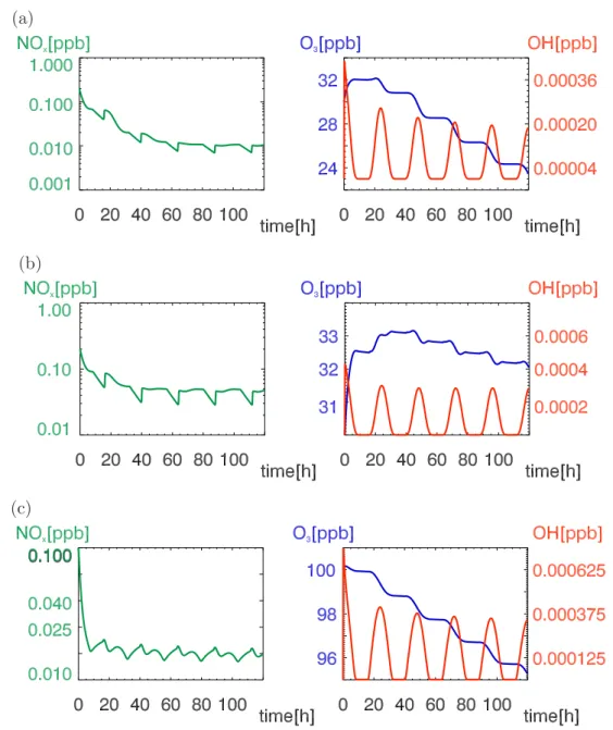
4.1 Mixing ratios for NO

, O

, and OH (scenarios LAND, MA- RINE and FREE) . . . 34 4.2 Mixing ratios for NO

, O

, and OH (scenarios PLUME, UR-

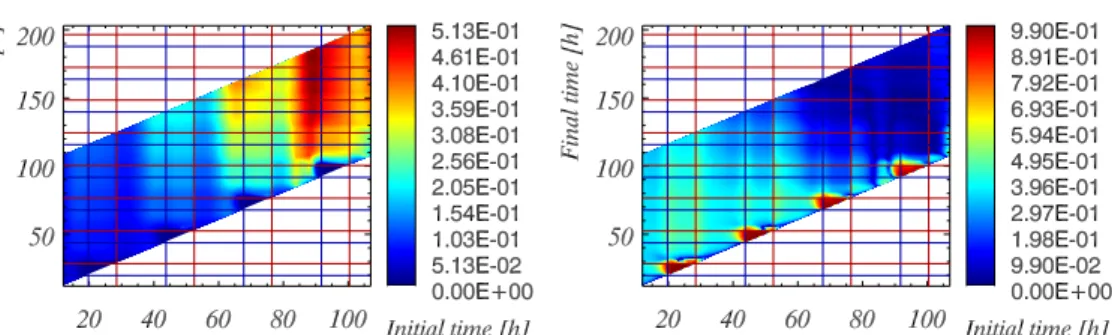
BAN and URBAN/BIO) . . . 35 4.3 Schematic presentation of the temporal singular vector dia-

gram (TSVD) . . . 36 4.4 Maximal grouped error growth with respect to initial uncer-

tainties (scenario LAND) . . . 38 4.5 TSVD of optimal grouped singular vectors with respect to

initial uncertainties (scenarios MARINE, FREE and PLUME) 39 4.6 Statistics of optimal grouped singular vectors with respect to

initial uncertainties for categories C

and C

(scenario MARINE) 41 4.7 Statistics of optimal grouped singular vectors with respect to

initial uncertainties for categories C

and C

(sce- nario MARINE) . . . 41 4.8 HC8- and ISO-sections of the TSVD of optimal projected sin-

gular vectors with respect to initial uncertainties (scenario MARINE) . . . 44 4.9 Statistics of optimal projected singular vectors with respect to

initial uncertainties for categories C

(scenario MARINE) 44 4.10 Maximal grouped relative error growth with respect to initial

uncertainties (scenario PLUME) . . . 47

LIST OF FIGURES v

4.11 TSVD of optimal grouped relative singular vectors with re- spect to initial uncertainties (scenarios PLUME and URBAN) 48 4.12 KET- and NO

-sections of the TSVD of optimal projected

relative singular vectors with respect to initial uncertainties (scenario URBAN) . . . 50 4.13 Statistics of optimal projected relative singular vectors with

respect to initial uncertainties for day 1 and night 1 of cate- gories C

and C

(scenario URBAN) . . . 51 4.14 Maximal grouped relative error growth with respect to emis-

sion uncertainties (scenario URBAN) . . . 54 4.15 TSVD of optimal grouped relative singular vectors with re-

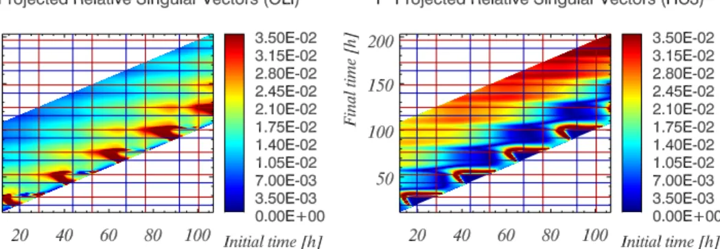
spect to emission uncertainties (scenarios PLUME and URBAN) 55 4.16 OLI- and HC3-sections of the TSVD of optimal projected rel-

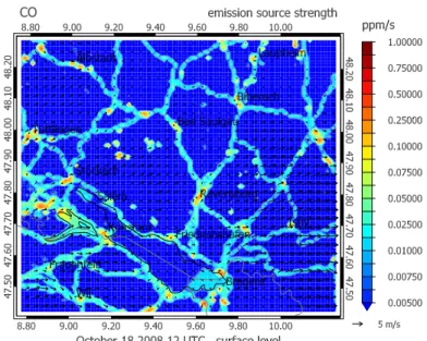
ative singular vectors with respect to emission uncertainties (scenario PLUME) . . . 56 5.1 CO emission source strength (ZPS-grid) . . . 65 5.2 Optimal horizontal placement of measurements of passive tracer

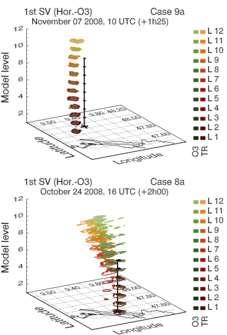
and ozone with respect to initial uncertainties (case 9a and case 8a) . . . 68 5.3 Optimal vertical placement of measurements of passive tracer

and ozone with respect to initial uncertainties (case 2a, case 5b, case 7a and case 10) . . . 70 5.4 Initial concentrations and optimal horizontal placement of mea-

surements with respect to initial uncertainties of O

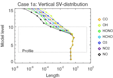
and NO at surface level (case 6) . . . 71 5.5 Optimal vertical placement of measurements of chemical com-

pounds with respect to initial uncertainties (case 1a) . . . 72 5.6 Relative ranking of the effect of initial uncertainties of O

and

CO for level 1 and level 9 . . . 74 5.7 Optimal horizontal placement of measurements with respect

to both emissions and initial uncertainties of HCHO at surface level (case 5a) . . . 76 5.8 Relative ranking of the effect of emission uncertainties of NO,

NO

, HCHO and CO at surface level . . . 77 5.9 Location dependent rankings of the effect of emission uncer-

tainties of HCHO at surface level (case 2a) . . . 78

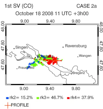
5.10 Location dependent rankings of the effect of emission uncer- tainties of CO at surface level (case 2a) . . . 79 A.1 Statistics of optimal projected relative singular vectors with

respect to initial uncertainties for categories C

and C

(scenario PLUME) . . . 106 A.2 Statistics of optimal projected relative singular vectors with

respect to initial uncertainties for categories C

and C

(scenario URBAN) . . . 107 A.3 Statistics of optimal projected relative singular vectors with

respect to initial uncertainties for categories C

and C

(scenario BIO) . . . 108 B.1 Optimal placement of measurements with respect to initial

uncertainties (case 1a) . . . 113 B.2 Optimal placement of measurements with respect to initial

uncertainties (case 1b) . . . 114 B.3 Optimal placement of measurements with respect to initial

uncertainties (case 2a) . . . 114 B.4 Optimal placement of measurements with respect to initial

uncertainties (case 2b) . . . 114 B.5 Optimal placement of measurements with respect to initial

uncertainties (case 3) . . . 115 B.6 Optimal placement of measurements with respect to initial

uncertainties (case 4a) . . . 115 B.7 Optimal placement of measurements with respect to initial

uncertainties (case 4b) . . . 115 B.8 Optimal placement of measurements with respect to initial

uncertainties (case 5a) . . . 116 B.9 Optimal placement of measurements with respect to initial

uncertainties (case 5b) . . . 116 B.10 Optimal placement of measurements with respect to initial

uncertainties (case 6) . . . 116 B.11 Optimal placement of measurements with respect to initial

uncertainties (case 7a) . . . 117 B.12 Optimal placement of measurements with respect to initial

uncertainties (case 7b) . . . 117

LIST OF FIGURES vii

B.13 Optimal placement of measurements with respect to initial uncertainties (case 8a) . . . 117 B.14 Optimal placement of measurements with respect to initial

uncertainties (case 8b) . . . 118 B.15 Optimal placement of measurements with respect to initial

uncertainties (case 9a) . . . 118 B.16 Optimal placement of measurements with respect to initial

uncertainties (case 9b) . . . 118 B.17 Optimal placement of measurements with respect to initial

uncertainties (case 10) . . . 119 B.18 Relative ranking of the effect of initial uncertainties of NO and

NO

for level 1, level 3, level 5, level 7 and level 9 . . . 120 B.19 Relative ranking of the effect of initial uncertainties of HCHO

and CO for level 1, level 3, level 5, level 7 and level 9 . . . 121 B.20 Relative ranking of the effect of initial uncertainties of HONO

and OH for level 1, level 3, level 5, level 7 and level 9 . . . 122 B.21 Location dependent rankings of the effect of emission uncer-

tainties of HCHO and CO (case 1a and case 1b) . . . 123 B.22 Location dependent rankings of the effect of emission uncer-

tainties of HCHO and CO (case 2a, case 3, and case 4a) . . . . 124 B.23 Location dependent rankings of the effect of emission uncer-

tainties of HCHO and CO (case 4b, case 5a, and case 5b) . . . 125 B.24 Location dependent rankings of the effect of emission uncer-

tainties of HCHO and CO (case 6, case 7a, and case 7b) . . . 126 B.25 Location dependent rankings of the effect of emission uncer-

tainties of HCHO and CO (case 8a, case 8b, and case 9a) . . . 127 B.26 Location dependent rankings of the effect of emission uncer-

tainties of HCHO and CO (case 9b and case 10) . . . 128

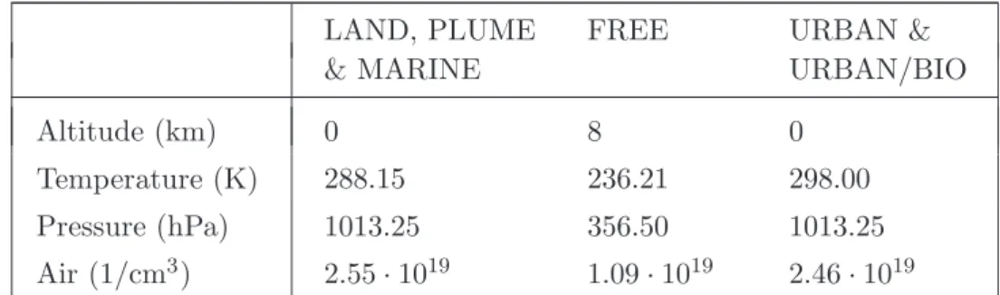
4.1 Meteorological parameters (tropospheric chemistry scenarios) . 32 4.2 Initial mixing ratios for the gas-phase constituents (tropo-

spheric chemistry scenarios) . . . 32

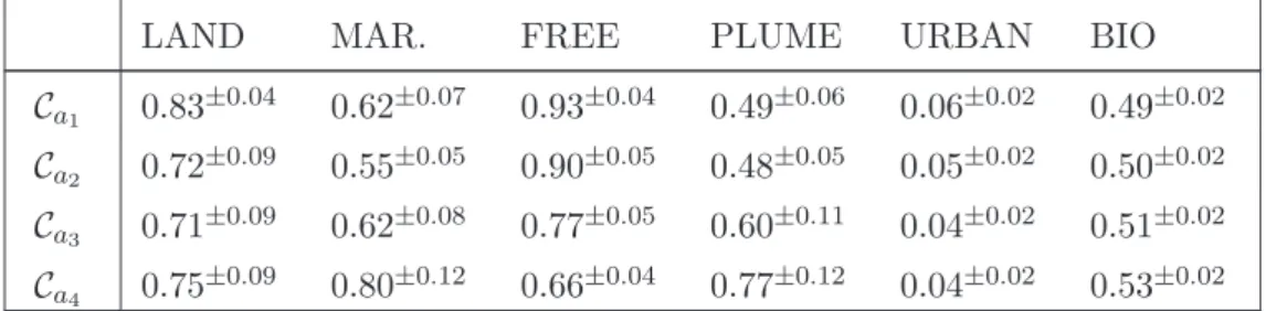
4.3 Statistics of NO

-sections of optimal grouped singular vectors with respect to initial uncertainties for categories C

(tro- pospheric chemistry scenarios) . . . 42

4.4 Statistics of NO

-sections of optimal grouped singular vectors with respect to initial uncertainties for categories C

(tro- pospheric chemistry scenarios) . . . 42

5.1 List of ZEPTER-2-flights . . . 59

5.2 List of ZEPTER-2 singular vector simulations . . . 62

5.3 Vertical grid structure of EURAD-IM (ZPS-domain) . . . 63

5.4 Singular values with respect to both emissions and initial un- certainties . . . 80

A.1 RADM2 species list . . . 85

A.2 Photolysis-Parameter (scenarios LAND, MARINE, PLUME, URBAN, and URBAN/BIO) . . . 88

A.3 Photolysis-Parameter (scenario FREE) . . . 89

A.4 Emission strength (tropospheric chemistry scenarios) . . . 90

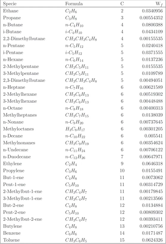
A.5 Emitted VOC compounds (tropospheric chemistry scenarios) . 91

LIST OF TABLES ix

A.6 Statistics of VOC compounds of optimal projected singular vectors with respect to initial uncertainties for category C

(scenarios LAND, MARINE, and FREE) . . . 93 A.7 Statistics of VOC compounds of optimal projected singular

vectors with respect to initial uncertainties for category C

(scenarios PLUME, URBAN, and BIO) . . . 94 A.8 Statistics of VOC compounds of optimal projected singular

vectors with respect to initial uncertainties for categories C

(scenario LAND) . . . 95 A.9 Statistics of VOC compounds of optimal projected singular

vectors with respect to initial uncertainties for categories C

(scenario MARINE) . . . 96 A.10 Statistics of VOC compounds of optimal projected singular

vectors with respect to initial uncertainties for categories C

(scenario FREE) . . . 97 A.11 Statistics of VOC compounds of optimal projected singular

vectors with respect to initial uncertainties for categories C

(scenario PLUME) . . . 97 A.12 Statistics of VOC compounds of optimal projected singular

vectors with respect to initial uncertainties for categories C

(scenario URBAN) . . . 98 A.13 Statistics of VOC compounds of optimal projected singular

vectors with respect to initial uncertainties for categories C

(scenario BIO) . . . 99 A.14 Statistics of VOC compounds of optimal projected singular

vectors with respect to initial uncertainties for category C

(scenarios LAND, MARINE, and FREE) . . . 100 A.15 Statistics of VOC compounds of optimal projected singular

vectors with respect to initial uncertainties for category C

(scenarios PLUME, URBAN, and BIO) . . . 101 A.16 Statistics of VOC compounds of optimal projected singular

vectors with respect to initial uncertainties for categories C

(scenario LAND) . . . 101 A.17 Statistics of VOC compounds of optimal projected singular

vectors with respect to initial uncertainties for categories C

(scenario MARINE) . . . 102

A.18 Statistics of VOC compounds of optimal projected singular vectors with respect to initial uncertainties for categories C

(scenario FREE) . . . 103 A.19 Statistics of VOC compounds of optimal projected singular

vectors with respect to initial uncertainties for categories C

(scenario PLUME) . . . 104 A.20 Statistics of VOC compounds of optimal projected singular

vectors with respect to initial uncertainties for categories C

(scenario URBAN) . . . 105 A.21 Statistics of VOC compounds of optimal projected singular

vectors with respect to initial uncertainties for categories C

(scenario BIO) . . . 105

B.1 RACM-MIM species list . . . 109

CHAPTER 1

Introduction

It is a typical feature that measurements of the earth’s environment have sparse temporal and spatial density and hence provide only incomplete snap- shots of the state of the system. This applies to both in situ observations and retrievals from space borne sensors. Consequently, an optimized configura- tion of available observation capabilities has to be considered to improve the information content of our monitoring capabilities. Adaptive observations of selected parameters in well defined targeted areas can reduce uncertainty and decrease forecast errors (Buizza et al. [2007]). Target areas for most valuable observations are sensitive system states, where small variations of considered input parameters lead to a significant forecast change.

The optimal adaption of observations is a frequently investigated problem in

numerical weather prediction. A classical topic are cases of explosive cyclo-

genesis at the North American east coast, which are often of highest rele-

vance for European weather development and its forecast. Various strategies

for targeting observations have been introduced, namely adjoint-sensitivity

(Buizza and Montani [1999]), ensemble transformation (Bishop and Toth

[1998]), statistical design (Berliner et al. [1998]), the breeding method (Toth

and Kalnay [1993]), Lyapunov vectors (e.g., Parker and O.Chua [1989]) and

singular vectors (Buizza and Palmer [1993]). In general, the denoted meth-

ods use a linear approach to evolve the uncertainties in time, even though

the forecast involves nonlinear systems. Singular vectors of the tangent lin-

ear model identify the directions of fastest perturbation growth over a finite

time interval. Their application to numerical weather prediction was in- troduced by Lorenz [1965], who estimated the atmospheric predictability of an idealized model by computing the largest error growth. Because of the high computational expenditure, singular vector analyses were applied to realistic meteorological problems only in the late 1980’s. Since the largest singular vectors contain the directions of fastest error growth (Buizza and Palmer [1993]), they are applied as reasonable tools to initialize ensemble forecasts. Their successful use in the ECMWF Ensemble Prediction System resulted in the first application of targeted singular vectors in a field campaign (Buizza and Montani [1999]). Several other field campaigns followed, in- cluding FASTEX (Fronts and Atlantic Storm-Track Experiment), NORPEX (North-Pacific Experiment), CALJET (California Land-falling JETs Exper- iment), the Winter Storm Reconnaissance Programs (WSR99 /WSR00) and NATReC (North Atlantic THORPEX Regional Campaign). Buizza et al.

[2007] investigated the results of the latter campaigns and stated that tar- geted observations are more valuable than observations taken in random areas. However, the extend of the impact is strongly dependent on regions, seasons, static observing systems, and prevailing weather regimes. Since sin- gular vector analysis is a well-established method within numerical weather prediction and is proven to be valuable, it is used as analysis method in this work.

The studies described above are dealing with perturbations of meteorological parameters. In atmospheric chemistry, studies attending targeted observa- tions are rare. The earliest stimulus for analyzing uncertainties of the chem- ical composition was provided by Khattatov et al. [1999]. By investigation of the linearized model, Khattatov inferred, that a linear combination of 9 initial species’ concentrations is sufficient to adequately forecast the concen- trations of the complete set of 19 simulated species 4 days later. Since most instruments measure concentrations of individual species, the determination of linear combinations has only limited practical value. Yet, Khattatov et al.

[1999] motivated to further examine the sensitivity of the initial chemical composition. Sandu et al. [2006] used singular vectors to estimate optimal adaptive measurements for chemical compounds. In this manner, application of the results to measurement strategies is feasible, as already demonstrated in the meteorological campaigns mentioned above. However, Sandu et al.

[2006] especially focused on the optimal placement of observations, while the

question which species are to be measured with priority remains mainly dis-

regarded. In contrast, the intention of the present work goes beyond local

optimization and furthermore addresses the problem of optimization with re-

gard to species. Unfortunately, adaptive observations of initial values get less

3

valuable with growing simulation length. Meanwhile, the effect of emission rates on the final concentration increases. Therefore, singular vector analysis is not only applied with regard to initial values, but moreover with regard to emission rates.

In summary, the present work seeks to give insight into the impact of uncer- tainties in emission strengths and initial species concentrations. Its objective is the detection of sensitive locations and species for atmospheric chemistry transport models, i.e. to answer the following questions:

Which chemical species have to be measured with priority?

Where is the optimal placement for observations of these components?

In addition, the calculated directions of largest error growth can be utilized for sensitivity studies, to initialize ensemble-forecasts, and to form chemical covariances.

This study is organized as follows: The theory of singular vector analysis is presented in chapter 2, where the application on initial uncertainties and emission factors is described as well as newly introduced special operators.

Singular vector analysis is implemented into a zero-dimensional model and

into a 3-dimensional model. While the zero-dimensional model only takes the

chemical kinetics into account, the 3-dimensional model additionally consid-

ers transport processes. In chapter 3 the setup of the adapted models is

summarized. The zero-dimensional model is applied to analyze several tro-

pospheric scenarios in chapter 4. Studies with the 3-dimensional model are

described in chapter 5. Finally, the results of this work are summarized in

chapter 6.

CHAPTER 2

Singular vector analysis

The singular vector analysis applied to a forecast model identifies sensitive system state modifications, where small variations of initial conditions lead to significant forecast changes. The leading singular vector reveals the direc- tion of fastest perturbation growth during a finite time interval.

In this work the singular vector analysis was applied to atmospheric chem- ical modeling to study the influence of chemical initial concentrations and emissions on the temporal evolution of chemical compounds. In section 2.1 emphasis is placed on initial uncertainties, while in section 2.2 emission fac- tors are addressed. These two parameters have been chosen since they both strongly determine the system’s evolution. Meteorological fields, deposition velocities, and boundary conditions are other parameters, to which the evo- lution of chemical species is sensitive, but they go beyond the scope of this study.

2.1 Uncertainties of initial values

Deterministic chemical forecasts propagate the concentrations of chemical species c ∈ R

(denoted in mass mixing ratios) forward in time. With M

denoting the model operator starting at initial time t

and ending at final time t

, the model solution reads:

c(t

) = M

c(t

). (2.1)

Since chemistry-transport models rely on initial values, which do not exactly match the true chemical state, the initial values have initial errors or uncer- tainties δc(t

). The problem of finding the most unstable initial uncertainty δc(t

) can be envisaged as the search of the phase space direction δc(t

) which results in maximum error growth.

By applying a first-order Taylor series approximation, the disturbed initial state evolves as follows:

M

[c(t

) + δc(t

)] = M

c(t

) + ∂M

∂c

c(tI)

δc(t

) + O [δc(t

)

]. (2.2)

Due to the fact, that the term

L

:= ∂ M

∂c

(tI)

(2.3) is linearized at the reference trajectory c(t) = M

c(t

) ∀ t ∈ [t

, t

], L

is termed the tangent-linear model. Considering initial errors sufficiently small to evolve linearly within a given time interval, terms of quadratic or higher order can be neglected:

M

[c(t

) + δc(t

)] ≈ M

c(t

) + L

δc(t

), (2.4) and the evolution of initial uncertainties can be described with the tangent linear model dynamics:

δc(t

) = L

δc(t

). (2.5) For more details on the derivation of equation (2.5) see, for example, Kalnay [2003]. The ratio between perturbation magnitudes at final time t

and initial time t

can be used to define a measure of error growth g(δc(t

)):

g(δc(t

)) := kδc(t

)k

kδc(t

)k

(2.6) (see Sandu et al. [2006] for a comprehensive discussion). Substituting the definition of the Euclidean norm in (2.6) leads to

g(δc(t

)) = s

δc(t

)

δc(t

)

δc(t

)

δc(t

) . (2.7)

2.1 Uncertainties of initial values 7

Maximizing this ratio with respect to the initial disturbance δc(t

) provides the direction of maximal error growth δc(t

). As g(δc(t

)) ≥ 0, the ini- tial perturbation δc(t

) that maximizes the squared error growth g

(δc(t

)), maximizes the error growth g(δc(t

)) as well. For convenience the squared error growth is treated henceforth:

δc

max

g

(δc(t

)) = max

δc(tI)6=0

δc(t

)

δc(t

)

δc(t

)

δc(t

) . (2.8) Using equation (2.5) the variable δc(t

) may be eliminated from the maxi- mization problem to leave

δc

max

g

(δc(t

)) = max

δc(tI)6=0

δc(t

)

L

L

δc(t

)

δc(t

)

δc(t

) . (2.9) The operator L

denotes the adjoint model of the tangent-linear operator L

. The adjoint K

of a real operator K is defined by the property

hKx, yi = hx, K

yi ∀ x, y ∈ R

, (2.10) where K

identifies the transpose operator and h., .i denotes the canonical Euclidean scalar product (e.g., Kalnay [2003]). The operator L

L

is also known as Oseledec operator. Obviously it is symmetric. Hence the ratio (2.9) is a Rayleigh quotient.

Rayleigh’s principle

For a symmetric matrix A ∈ R

, a Rayleigh quotient r

(A; x) with x ∈ R

is defined as

r

(A; x) := x

A x

x

x , x 6= 0. (2.11)

Let λ

≥ λ

≥ ... ≥ λ

be the eigenvalues of A and v

the associated eigen- vectors. Rayleigh’s principle states that a Rayleigh quotient r

(A; x) reaches its maximum λ

when v

is inserted (Noble and Daniel [1969]). Furthermore, for a symmetric matrix A ∈ R

and a symmetric positive-definite matrix B ∈ R

, a fraction of the type

r

(A, B; x) := x

A x

x

B x , x 6= 0 (2.12)

is referred to as generalized Rayleigh quotient r

(A, B; x). With the trans-

formation C = B

AB

, y = B

x the generalized Rayleigh quotient

r

(A, B; x) can be reduced to a Rayleigh quotient r

= (C; y) and Rayleigh’s

principle can be applied. Since various Rayleigh quotients will be considered in this section, notations (2.11) and (2.12) are adapted to

r(D; x) := x

D

D x

x

x , x 6= 0 (2.13)

and

r

(D, E; x) := x

D

D x

x

E

E x , x 6= 0 (2.14) to describe the subsequent problems more compactly. Thereby D

D and E

E have to be symmetric (which holds for every D ∈ R

, E ∈ R

) and E

E, moreover, has to be positive-definite. For the new definitions, the transformation of the generalized Rayleigh quotient into a Rayleigh quotient changes to:

r

(D, E; x) = r(G; y), G = DE

, y = E x. (2.15) The maximal value of the Rayleigh quotient r(D; x) (2.14) is the largest eigenvalue λ

of the matrix D

D. Accordingly, its assigned eigenvector v

maximizes the fraction r(D; x).

Applying Rayleigh’s principle to problem (2.9) results in searching for the largest eigenvalue λ

and the assigned eigenvector v

(t

) of the following eigenvalue problem:

L

L

v(t

) = λ v(t

). (2.16) Since the entire set of eigenvectors v

(t

) of L

L

can be chosen to form an orthonormal basis in the n-dimensional tangent space of linear per- turbations, the eigenvectors v

(t

), i=2,...,n define secondary directions of instability. The amount of influence of eigenvector v

(t

) is defined by the magnitude of the square root of the associated eigenvalue λ

.

The name singular vector analysis refers to the fact, that the square roots of the eigenvalues λ

of L

L

are the singular values σ

of the tangent- linear model L

. The associated left and right singular vectors u

(t

) ∈ R

and v

(t

) ∈ R

of the operator L

are defined satisfying the following con- ditions:

L

v

(t

) = σ

u

(t

) and (2.17) L

u

(t

) = σ

v

(t

), (2.18) with kvk

=1 and kuk

=1. Combining these two equations

L

L

v

(t

) = σ

L

u

(t

) = σ

v

(t

) (2.19)

2.1 Uncertainties of initial values 9

reveals that the eigenvectors v

(t

) of the Oseledec operator are the right sin- gular vectors of the tangent-linear operator L

. Hence, the right singular vector v

(t

) assigned to the largest singular value σ

of a chemistry-transport model characterizes the direction of maximum error growth over a finite time interval [t

, t

]. The singular value σ

is the maximum value of the original ratio (2.6) and defines the amount of error growth.

2.1.1 Relative error growth

Since concentrations of different species may vary by many orders of magni- tude, perturbations of species with larger concentrations or higher reactivity are expected to dominate the error growth. To avoid this effect and gain a relative error growth, the absolute uncertainties δc(t) ∀ t ∈ [t

, t

] are scaled by current concentrations c(t) ∀ t ∈ [t

, t

]. For this purpose, a weight matrix W

∈ R

,

W

:= diag c

(t)

i,j,k,s

∀ t ∈ [t

, t

] (2.20) is introduced, which assigns the concentration of chemical species s to each grid point (i, j, k). Its application provides the relative error δc

∈ R

δc

(t) := W

δc(t) ∀ t ∈ [t

, t

] (2.21) as well as the relative error growth g

with

g

(δc

(t

)) := kδc

(t

)k

kδc

(t

)k

= kW

δc(t

)k

kW

δc(t

)k

(2.22) (Sandu et al. [2006]). Applying the squared measure and expressing the final perturbation in terms of the initial perturbation

δc

(t

) = W

δc(t

) = W

L

δc(t

) (2.23) leads to a generalized Rayleigh quotient with respect to δc(t

):

g

(δc

(t

)) = r

(B, W

; δc(t

)),

where B : = W

L

. (2.24) By formula (2.15) the generalized Rayleigh quotient (2.24) is transformed into a Rayleigh quotient

g

(δc

(t

)) = r(B

; δc

(t

)),

where B

: = B W

= W

L

W

, (2.25)

and Rayleigh’s principle can be applied. Thus the phase space direction δc

(t

), for which the ratio (2.25) gains its maximal value, is the solution v

(t

) of the symmetric eigenvalue problem

B

B

v

(t

) = λ

v

(t

)

with v

(t

) : = W

v(t

) (2.26) assigned to the largest eigenvalue λ

. Comparing problem (2.26) with the original problem (2.16), it is readily seen that the solution v

(t

) ∈ R

is the right singular vector of the operator B

and the square root of the eigenvalue λ

is the associated singular value σ

. Due to this property the singular vector v

(t

) is called relative singular vector henceforth.

2.1.2 Projected error growth

Another central aim is to examine the error growth of a limited set of chem- ical species for limited geographical regions. To fulfill this requirement a projection operator P

∈ R

is applied, which sets the entries of the per- turbations to zero outside the focused species and regions (Barkmeijer et al.

[1998]). Thus the projection operator is a diagonal matrix with binary en- tries, dependent on the spatial or chemical feature of interest. The projection operator reads

P

:= diag (p

)

, p

=

( 1 ∀ i ∈ P(t)

0 otherwise , (2.27)

where P (t) denotes the set of selected chemical compounds and grid locations at time t. Using the example of n=5 and P (t)={2, 4, 5}, the projection operator is given by

P

=



 

 



0 0 0 0 0 0 1 0 0 0 0 0 0 0 0 0 0 0 1 0 0 0 0 0 1



 

 

 .

Note, that set P (t) and projection operator P

are time-dependent. They may differ at initial and final time.

In order to consider the impact of a limited perturbation at initial time t

on a limited perturbation at time t, the projected error δc

∈ R

is defined as

δc

(t) := P

L

P

δc(t

). (2.28)

2.1 Uncertainties of initial values 11

In case, that there is no limitation of regions and species at time t, t ∈ [t

, t

], the projection operator P

equals the identity matrix. Since the projection operator is idempotent and L

= I, the projected error at initial time reads δc

(t

) = P

L

P

δc(t

) = P

δc(t

). (2.29) After explicit use of equation (2.29), the projected error at final time becomes δc

(t

) = P

L

δc

(t

). (2.30) Application of equation (2.29) and equation (2.30) amounts to the projected error growth g

:

g

(δc

(t

)) := kδc

(t

)k

kδc

(t

)k

= kP

L

P

δc(t

)k

kP

δc(t

)k

. (2.31)

The squared projected error growth reduces to a Rayleigh quotient g

(δc

(t

)) = r(B; δc

(t

)),

where B : = P

L

, (2.32) subject to

[δc

(t

)](j) = [P

δc(t

)](j ) =

( [δc(t

)](j) ∀ j ∈ P

0 otherwise. (2.33)

Here, [x](j) denotes the j-th component of a vector x. According to Rayleigh’s principle, the phase space direction that maximizes the Rayleigh quotient (2.43) is the solution v

(t

) of the symmetric eigenvalue problem

B

B v

(t

) = λ

v

(t

) (2.34) assigned to largest eigenvalue λ

. However, the solution v

(t

) does not necessarily ensure condition (2.33). In order to grant condition (2.33), the so- lution space has to be restricted. Therefore, equation (2.34) is left-multiplied with P

at first:

P

B

B v

(t

) = λ

P

v

(t

). (2.35) Application of

P

v

(t

) = v

(t

) (2.36) yields

B

B

v

(t

) = λ

v

(t

),

with B

: = B P

= P

L

P

. (2.37)

Here, the solution v

(t

) assigned to the largest eigenvalue λ

holds the required restriction (2.33). The eigenvector v

(t

) ∈ R

is the right singular vector of the operator B

and therefore it is referred to as projected singular vector. The square root of the eigenvalue λ

is the associated projected singular value σ

.

Furthermore, it is possible to combine the projected error (2.28) with the relative error (2.21), yielding the projected relative error δc

(t):

δc

(t) := W

δc

(t). (2.38) Hence, the projected relative error growth g

(δc

(t

)) is given by:

g

(δc

(t

)) := kδc

(t

)k

kδc

(t

)k

= kW

P

L

P

δc(t

)k

kW

P

δc(t

)k

. (2.39) After explicit use of

δc

(t

) = W

P

L

δc

(t

), (2.40) the squared projected relative error growth reads as a generalized Rayleigh quotient:

g

(δc

(t

)) = r

(B, W

; δc

(t

)), (2.41) where B : = W

P

L

. (2.42) Use of transformation (2.15) reduces the generalized Rayleigh quotient into a Rayleigh quotient

g

(δc

(t

)) = r(BW

; δc

(t

)) (2.43) subject to

[δc

(t

)](j) = [W

δc

(t

)](j ) =

( [

](j) ∀ j ∈ P

0 otherwise. (2.44)

The phase space direction that maximizes the Rayleigh quotient (2.43), is the solution v

(t

) of the symmetric eigenvalue problem

W

B

B W

v

(t

) = λ

v

(t

)

with v

(t

) : = W

v

(t

) (2.45) assigned to the largest eigenvalue λ

. Since the solution v

(t) needs to hold condition (2.44), the solution space has to be restricted. Therefore, the eigenvalue problem is restated by multiplying with P

:

P

W

B

B W

v

(t

) = λ

P

v

(t

). (2.46)

2.1 Uncertainties of initial values 13

The new generalized eigenvalue problem ensures that condition (2.44) holds.

In order to reduce the general eigenvalue problem to a symmetric eigenvalue problem (which is requested for the power method, see section 3.3.1) fur- ther modifications have to be made. Application of the fact, that diagonal matrices of the same dimension commute, yields

P

v

(t

) = P

W

v

(t

)

= W

P

v

(t

) = W

v

(t

) = v

(t

). (2.47) Substituting relation (2.47) into equation (2.46) gives a symmetric eigenvalue problem:

B

B

v

(t

) = λ

v

(t

),

where B

: = W

P

L

W

P

. (2.48) The solution v

(t

) ∈ R

assigned to the largest eigenvalue λ

of the final eigenvalue problem (2.48) is referred to as projected relative singular vector, since it is the right singular vector of the operator B

. The square root of the eigenvalue λ

is the associated projected relative singular value σ

.

2.1.3 Grouped error growth

So far, the effect of each species was regarded independently. Instead of examining the initial disturbances individually, one can also decide to look at the influence of groups of chemical species, which chemically act in a similar manner. To the knowledge of the author this problem has not been addressed in the context of singular vector analysis previously. In order to implement this new approach, a family operator F

∈ R

is introduced.

Let F

(t) represent one of f (t) pairwise disjoint families with m

(t) members.

Adopting the convention that A(i, j) refers to the entry that lies in the i-th row and the j-th column of a matrix A, each entry of the family operator reads

F

(i, j )

=

( 1 / m

(t) ∀ i, j ∈ F

(t)

0 otherwise. (2.49)

Note, that each chemical species is only allowed to belong to one family, i.e.

f

\

k=1

F

(t) = ∅ . (2.50)

An example of a family operator at initial time t

is

F

=



 

 

 



1/2 0 0 0 1/2 0

0 1/3 0 1/3 0 1/3

0 0 0 0 0 0

0 1/3 0 1/3 0 1/3

1/2 0 0 0 1/2 0

0 1/3 0 1/3 0 1/3



 

 

 



, (2.51)

where n = 6, f (t

) = 2, m

(t

) = 3, m

(t

) = 2, F

(t

) = {2, 4, 6} and F

(t

) = {1, 5}. If each family has only one member, the family operator equals the projection operator with P (t) = S

k=1

F

(t). The family operator is time dependent, hence the user can focus on distinct families at different times.

The influence of a set of chemical groups at initial time t

on another set of chemical groups at time t is determined by the grouped error:

δc

(t) := F

L

F

δc(t

). (2.52) If no chemical group is considered at time t, t ∈ [t

, t

], the family operator F

equals the identity matrix. With the aid of the idempotence of the family operator and L

= I, the grouped error at initial time reduces to

δc

(t

) = F

L

F

δc(t

) = F

δc(t

). (2.53) Substituting the grouped error (2.52) into the measure of error growth gives

g

(δc

(t

)) := kδc

(t

)k

kδc

(t

)k

= kF

L

F

δc(t

)k

kF

δc(t

)k

. (2.54) After use of

δc

(t

) = F

L

δc

(t

), (2.55) the squared ratio becomes a Rayleigh quotient

g

(δc

(t

)) = r(B; δc

(t

)),

with B : = F

L

, (2.56) subject to

[δc

(t

)](j) = (

mk

P

i∈Fk(tI)

[δc(t

)](i) ∀ j ∈ F

(t

)

0 otherwise. (2.57)