Diplomarbeit
Boundary behavior of singular integrals
ausgeführt am Institut für
Analysis und Scientic Computing
der Technischen Universität Wien
unter der Anleitung von
Ao.Univ.Prof. Dr. Harald Woracek
durch
Monika Pichler
2860 Kirchschlag, Stang 32, Österreich.
6. Mai 2013
Preface
Let µ be a complex Borel measure on the unit circle. In this work we study integral transforms ofµ on the unit disk, namely the well-known Cauchy transform as well as the closely related Poisson and conjugate Poisson transforms. These transforms are of partic- ular interest in function theory, as certain classes of analytic functions allow for integral representations of this type, and they are important tools in many function theoretic proofs.
We are concerned with the behavior of the transforms near the support of the measure µ. In the case of measures absolutely continuous with respect to Lebesgue measure on the circle, this topic has been thoroughly studied. The results are well-known and can be found for instance in [10].
If the measureµis singular with respect to Lebesgue measure, its Cauchy transform tends to innity as the function argument approaches points lying in the support of the measure.
The mode of growth of the transforms in this case became the object of deeper study very recently. In [2], A. Poltoratski introduced a classication of measures based on the relative speed of growth of their Poisson and conjugate Poisson transforms. Several results on this subject have been published in the recent years, and there are a number of open questions at this point.
In this thesis we give an overview of the developments in this eld. In the rst chapter, we provide necessary denitions and preliminary results. Chapter 2 deals with the classical results on absolutely continuous measures.
In Chapter 3, we turn to the study of the normalized Cauchy transform of a measure, which is an operator dened on the space ofµ-integrable functions. The main result is a statement about the boundary behavior of the image functions of the normalized Cauchy transform that is due to A. Poltoratski [1]. In the rst two sections of this chapter, we present a construction that actually originates in a dierent direction of study but leads to important results on the normalized Cauchy transform, and was introduced by D.N. Clark [5] and taken up by A.B. Aleksandrov [6]. The rest of the chapter follows A. Poltoratski's paper [1].
In Chapter 4 it is shown how the results from Chapter 3 can be applied in the study of the boundary behavior of the Poisson and conjugate Poisson transforms of singular measures.
We present the classication from [2] and state some results characterizing those classes that were obtained by A. Poltoratski and P.W. Jones in [2], [3] and [4].
At this point I want to thank my advisor Harald Woracek for his support and helpful suggestions.
Vienna, May 2013
Contents
1 Preliminaries 3
1.1 The Hardy Spaces on the unit disk . . . 3
1.2 Harmonic functions . . . 4
1.3 Integral transforms of measures . . . 5
1.4 Further results . . . 6
2 Absolutely continuous measures 8 2.1 The symmetric derivative of a measure . . . 8
2.2 The Poisson transform . . . 13
2.3 The conjugate Poisson transform . . . 17
3 The normalized Cauchy transform 21 3.1 Inner functions and singular measures . . . 21
3.2 Construction of the unitary operator Uα . . . 27
3.3 Boundary behavior of functions in θ∗(Hp) . . . 32
3.4 The nontangential maximal function . . . 46
3.5 Boundary behavior of the normalized Cauchy transform . . . 48
4 Measures with singular components 57 4.1 Denition of the Classes I-IV . . . 57
4.2 Class I . . . 59
4.3 Class II . . . 62
4.4 Class III . . . 63
4.5 Class IV . . . 64
Chapter 1
Preliminaries
1.1 The Hardy Spaces on the unit disk
We use the following notational conventions throughout.
D:={z∈C:|z|<1} denotes the open unit disk,T:=∂Dis the unit circle.
M(T)denotes the set of all nite regular complex Borel measures onT, andM+(T)is the subset of all nite positive measures.
The normalized Lebesgue measure on the unit circle is denoted by σ, and speaking of absolutely continuous or singular measures we mean with respect to σ unless explicitly stated otherwise.
We introduce the Hardy Spaces on the unit disk: For0< p≤ ∞,Hp denotes the space of holomorphic functions onD which satisfy
kfkHp := sup
0<r<1
Z
T
|f(rξ)|pdσ(ξ)
1/p
<+∞, (1.1)
if0< p <∞, and in the casep=∞
kfkH∞ := sup
z∈D
|f(z)|<+∞, (1.2)
i.e.,H∞ is the space of bounded analytic functions in D.
Ifp≥1, the spaceHp is a Banach space, if0< p <1, it is a complete metric space. We state some properties of the functions lying in Hardy spaces that will be relevant in the following.
(i) Every functionf ∈Hp has boundary values almost everywhere onT, and the bound- ary function f˜lies in Lp(σ), with kfkHp = kf˜kLp. Thus Hp is isomorphic to a closed subspace ofLp(σ); see [13, Chapter II, Theorem 3.1]. Thanks to this correspondence, we will usually not distinguish betweenf ∈Hp and its boundary function in Lp(σ).
(ii) Let 1 ≤ p ≤ ∞. Then we have the following characterization of the elements of Hp in terms of their boundary function ([12, Theorem 4.25]): f ∈Lp(σ) is the boundary function of a function inHp if and only if for alln∈N
Z
T
ζnf(ζ)dσ(ζ) = 0. (1.3)
(iii) If1≤p≤ ∞, every functionf ∈Hp has the Cauchy representation f(z) =
Z
T
f(ξ)
1−zξ¯dσ(ξ), z∈D. (1.4)
(iv) We set H0p:=
f ∈Hp |f(0) = 0 and H0p:=
f ∈Lp(σ) |f¯∈H0p . In terms of boundary functions, these are the spaces (p≥1)
H0p =
f ∈Lp(σ) |(1.3)holds for alln∈N0 , (1.5) H0p =
f ∈Lp(σ) |(1.3)holds for alln≤0 . (1.6) If1< p <∞, we have the decomposition Lp(σ) =Hp⊕H0p, see e.g. [15, Chapter 9].
(v) The dual space ofHp,1< p <∞, can be identied withHq, whereqis the conjugate index ofp, i.e., the unique positive number such that 1p+1q = 1holds; see [14, Section 3.6].
The duality product forf ∈Hp and g∈Hq is given by hf, gi:=
Z
T
f(ξ)g(ξ)dσ(ξ).
1.2 Harmonic functions
A functionu which is continuous onDand twice continuously dierentiable onDis called harmonic if ∆u(x+iy) = ∂∂x2u2 + ∂∂y2u2 = 0 in D. We state some facts about harmonic functions we will need later on. Proofs of the statements can be found in [13], [17], [21, Chapter 11].
(i) Iff is a function continuous onDand analytic inD, and we writef(z) =u(z) +iv(z) with real-valueduand v, then uandv satisfy the Cauchy-Riemann dierential equations,
∂u
∂x = ∂v
∂y and ∂u
∂y =−∂v
∂x. (1.7)
From these equations we infer thatuand v are harmonic functions:
∂2u
∂x2 = ∂
∂x
∂v
∂y = ∂
∂y
∂v
∂x = −∂2u
∂y2,
∂2v
∂x2 = − ∂
∂x
∂u
∂y = − ∂
∂y
∂u
∂x = −∂2v
∂y2. By the linearity of the derivative,f itself is harmonic.
(ii) Conversely, every real-valued harmonic function u on D is the real part of some ana- lytic function on D. The corresponding imaginary part, which is then called a harmonic conjugate ofu, can be constructed from the Cauchy-Riemann dierential equations. Har- monic conjugates are unique up to a constant and we call a harmonic conjugatevsatisfying v(0) = 0the harmonic conjugate ofu.
(iii) For positive harmonic functions we have Harnack's inequality (see [22, Theorem 1.18]):
Theorem 1.2.1. Suppose thatu is positive and harmonic in the open ballUR(z0) :={z∈ C:|z−z0|< R}. Forz∈UR(z0), set r:=|z−z0|. Then the inequality
R−r
R+ru(ξ)≤u(z)≤ R+r
R−ru(ξ) (1.8)
holds.
1.3 Integral transforms of measures
Letµ∈M(T). We dene the Cauchy transformK[µ]ofµon the unit disk by K[µ] (z) :=
Z
T
1
1−ξz¯ dµ(ξ). (1.9)
The Cauchy transform is an analytic function inD. Moreover, it lies in the Hardy spaces Hp for p <1, see [19, Theorem 3.5].
We further dene the Poisson- and conjugate Poisson transform of µ, P[µ] and Q[µ], respectively, through
P[µ] (z) :=
Z
T
1− |z|2
|ξ−z|2dµ(ξ) = Z
T
P(z, ξ)dµ(ξ), (1.10)
Q[µ] (z) :=
Z
T
2Im ξz¯
|ξ−z|2 dµ(ξ) = Z
T
Q(z, ξ)dµ(ξ). (1.11)
Here,P(z, ξ) = 1−|z|2
|ξ−z|2 is the Poisson kernel, andQ(z, ξ) = 2Im(ξz¯ )
|ξ−z|2 is the conjugate Poisson kernel. These transforms are harmonic functions inD.
If µ ∈M(T) is a real-valued measure, its Poisson and conjugate Poisson transforms are real-valued harmonic functions. The name conjugate Poisson transform is due to the fact that in the case of a real-valued measure,Q[µ]is precisely the conjugate function ofP[µ]: The Poisson kernelP(z, ξ) is the real part of the function ξ+zξ−z, and the conjugate Poisson kernelQ(z, ξ) is its imaginary part. Hence we have
P[µ] (z) +iQ[µ] (z) = Z
T
ξ+z
ξ−zdµ(ξ), (1.12)
which is analytic inD. ObviouslyQ[µ]satises the condition Q[µ] (0) = 0.
For arbitrary complex measures, the Poisson and conjugate Poisson transform are not necessarily real-valued, but we still have (1.12), and also in this caseQ[µ]is called conjugate function ofP[µ].
Since1 +ξ+zξ−z = 1−2ξz¯ , we further have the relation K[µ] (z) = 1
2 Z
T
dµ+1
2P[µ] (z) + i
2Q[µ] (z) (1.13)
between the Cauchy and the Poisson and conjugate Poisson transforms ofµ.
1.4 Further results
We state some results here that are important tools in following proofs and give references on where to nd further details and proofs of the statements.
The rst statement is Fatou's jump theorem (see [14, Section 2.4]), which establishes a relation between boundary values onT of the Cauchy transform from inside and outside D. For, although we are mainly concerned with the Cauchy transform as a function on the unit disk, it is clearly dened forz ∈ Cˆ\T, where Cˆ := C∪ {∞}. If we set De := ˆC\D,¯ thenK[µ]is analytic on bothDand De and satisesK[µ] (∞) = 0.
We denote byHp(De),0< p≤ ∞, the set of all functionsF that are analytic onDe and for whichz 7→F(1/z) belongs toHp. The restriction K[µ]
De lies in the spaces Hp(De) for 0 < p < 1 and thus it has boundary values σ-almost everywhere on T from De. For more details on the Cauchy transform on De and the proof of the statement below see Section 2.4 of [14].
Theorem 1.4.1 Let µ∈M(T).Then, for σ-almost all ξ∈T,
r%1limK[µ] (rξ)−lim
r&1K[µ] (rξ) = dµ dσ(ξ).
In particular, if µ⊥σ, at σ-almost every point on T, we have the relation
r%1limK[µ] (rξ) = lim
r&1K[µ] (rξ). (1.14)
Kolmogorov's theorem provides us with a weak type estimate for the Cauchy transform of a measure; see [14, Theorem 3.4.1].
Theorem 1.4.2 Let µ∈ M(T). Then there exists a constant A >0 such that for every λ >0 the estimate
σ({|K[µ]|> λ})≤ Akµk
λ (1.15)
holds.
The following two statements are concerned with integral representations of harmonic functions by means of the Poisson transform and highlight the importance of this transform in harmonic function theory; see [12, Theorem 1.10, Theorem 1.5].
Theorem 1.4.3. Let u be a nonnegative harmonic function on D. Then there exists a measureµ∈M+(T) such that
u(z) = Z
T
P(z, ζ)dµ(ζ), z∈D. (1.16)
In addition, if a harmonic functionuis continuous on the boundary, the measure is explic- itly given as the absolutely continuous measure with densityu
T:
Theorem 1.4.4. Letu be harmonic onDand continuous onD. Thenu has the represen- tation
u(z) = Z
T
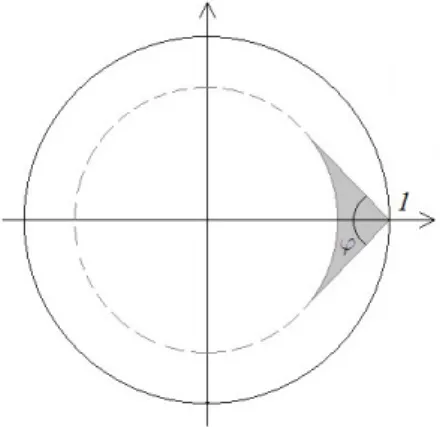
P(z, ζ)u(ζ)dσ(ζ), z∈D. (1.17) Let E be a subset of RN. We call a collection F of nontrivial closed balls a Besicovitch covering forE if everyx∈E is the center of a ballB(x)∈ F. For such coverings, we have the following Besicovitch covering theorem ([23, Chapter II, Theorem 18.1]).
Theorem 1.4.5. Let E ⊆RN be a bounded set, and let F be a Besicovitch covering for E. Then there exists a positive integer cN depending only on the dimension N such that there are cN subcollectionsB1, . . . ,BcN of F with the following properties:
(i) for every k= 1, . . . , cN, the collection Bk contains countably many disjoint balls;
(ii) E⊆
cN
S
k=1
S
B∈Bk
B.
Finally we state the Marcinkiewicz interpolation theorem ([13, Chapter I, Theorem 4.5]).
Theorem 1.4.6. Let (X, µ) and (Y, ν) be measure spaces, and let 1 < p ≤ ∞. Suppose that T is a map dened both on L1(X, µ) and Lp(X, µ) and mapping into the space of ν-measurable functions. Suppose further that T satises
(i) |T(f+g)| ≤ |T f|+|T g| on Y;
(ii) T is of weak type (1,1), i.e., for each λ >0 and f ∈L1(X, µ), ν({|T f|> λ})≤ A0kfkL1(X,µ)
λ ;
(iii) if p <∞, then T is of weak type (p,p), i.e., for each λ >0 and f ∈Lp(X, µ), ν({|T f|> λ})≤ A1kfkpLp(X,µ)
λp , and if p=∞, T satises
kT fkL∞(Y,ν)≤A1kfkL∞(X,µ).
Then for each1< p0< p, there is a constant Ap0 depending only onA0, A1, pandp0such that for allf ∈Lp0(X, µ)
kT fkLp0(Y,ν) ≤Ap0kfkLp0(X,µ).
Chapter 2
Absolutely continuous measures
In this chapter we concern ourselves with the boundary behavior of the Poisson and con- jugate Poisson transforms of an absolutely continuous measureµ∈M(T). We show that in this case, boundary values of both transforms exist almost everywhere on T. The rst part of the chapter is dedicated to the symmetric derivative and maximal function of a measure.
2.1 The symmetric derivative of a measure
Forξ ∈ Tand r ∈(0,2]we set Ir(ξ) := T∩Ur(ξ) = {η ∈T
|ξ−η|< r}, i.e., Ir(ξ) is an open subarc ofT centered inξ that is obtained by intersectingT with the open ball of radiusr ∈(0,2]centered at ξ.
Denition 2.1.1. Letµ∈M(T). We set
(Arµ) (ξ) := µ(Ir(ξ))
σ(Ir(ξ)), and (2.1)
(Dµ) (ξ) := lim
r→0(Arµ) (ξ), (2.2)
whenever this limit exists. (Dµ) (ξ) is called the symmetric derivative of µat ξ. Further- more, we dene the maximal function of the measureµby
(M µ) (ξ) := sup
0<r<∞
(Ar|µ|) (ξ), (2.3) where|µ|denotes the total variation ofµ.
We are going to show that if µ is absolutely continuous with respect to the Lebesgue measure, the symmetric derivative coincidesσ-almost everywhere with the Radon-Nikodym derivative ofµwith respect toσ, and that for a singular measureµthe symmetric derivative vanishes almost everywhere with respect toσ. First we establish some results about the maximal functionM µ.
Proposition 2.1.2. Let µ∈M(T) and K ∈(0,∞]. The function SKµ(ξ) := sup
0<r<K
(Ar|µ|) (ξ)
is lower semicontinuous, i.e., for everyλ∈R, the set {SKµ > λ}1 is open. In particular, the maximal functionM µis lower semicontinuous.
1Notation: this expression is an abbreviation denoting the set{ξ∈T| (SKµ) (ξ)> λ}.
Proof. Since SKµ depends only on the total variation of the measure, we may assume µ≥0. We xλ >0, denoteEλ :={SKµ > λ}and xξ∈Eλ. By the denition of the set, we ndr ∈(0, K) and t > λsuch that µ(Ir(ξ)) =tσ(Ir(ξ)). Furthermore, since t/λ >1 andσ is regular, there is someδ ∈(0, K−r) for whichσ(Ir+δ(ξ))< λtσ(Ir(ξ))holds.
Letη∈Iδ(ξ), then by the triangle inequality we haveIr(ξ)⊆Ir+δ(η). This yields, using the invariance ofσ under rotations,
µ(Ir+δ(η))≥µ(Ir(ξ)) =tσ(Ir(ξ))> λσ(Ir+δ(ξ)) =λσ(Ir+δ(η)),
and since r+δ < K, η lies in Eλ. As η ∈ Iδ(ξ) was arbitrary, we see that Iδ(ξ) ⊆ Eλ, hence the set is open.
We proceed with a statement about the possible size of the set where the maximal function M µis large. We will see thatM µcan take large values on relatively small sets only. First, we prove the following covering lemma.
Lemma 2.1.3. Given a nite set of arcsIj =Irj(ξj), j = 1, . . . , m, there exists a subset of indices J ⊆ {1, ..., m} such that
(i) the collection {Ij, j ∈J} is pairwise disjoint, (ii) Sm
j=1
Ij ⊆ S
j∈J
I3rj(ξj), and (iii) σ
m S
j=1
Ij
≤6P
j∈J
σ(Ij).
Proof. We order the arcs such that r1 ≥ r2 ≥ ... ≥rm. Now we inductively choose the indices in J in the following way: We set j1 = 1, then remove all Ij which intersect I1. We then choose the rst remaining index, if there are any remaining arcs, to be j2, and again remove all of the remaining arcs that intersect Ij2. Continuing in this way as long as possible, we arrive at a set of indices J = {j1, j2, ..., jk}. Clearly, the corresponding collection of arcs is disjoint. Furthermore, we note that every discarded arc I intersects someIj0 withj0 ∈J, whose radius rj0 is larger than that of I. ThusI is contained in the arc centered atξj0 with radius3rj0 by the triangle inequality. This proves (ii).
In order to prove the third statement, we rst derive an estimate of the σ-measure of some subarc of T with that of a smaller subarc: For r ∈ (0,2], a short calculation gives σ(Ir(ξ)) = π2arcsin r2
. We note that for suchr the inequality r2 <arcsin(r2)< r holds, which leads to the estimate
r
π ≤σ(Ir(ξ))≤ 2r π .
Considering now the arc centered at ξ with triple radius, we use the right part of this inequality to estimateσ(I3r(ξ))and then the left part forσ(Ir(ξ))and thereby obtain
σ(I3r(ξ))≤ 2
π3r≤6σ(Ir(ξ)). (2.4)
With this estimate, using (ii) we get σ
m
[
j=1
Ij
≤σ
[
j∈J
I3rj(ξj)
≤X
j∈J
σ I3rj(ξj)
≤6X
j∈J
σ(Ij).
Theorem 2.1.4. Letµ∈M(T). Then for every λ >0, the inequality
σ({M µ > λ})≤ 6kµk
λ (2.5)
holds, wherekµk=|µ|(T) is the total variation norm of µ.
Proof. We x λ > 0. As established in Proposition 2.1.2, Eλ := {M µ > λ} is an open set. Let K be a compact subset of Eλ. By the denition of M µ, for each ξ ∈ K we nd an arc Iξ = Irξ(ξ) such that |µ|(Iξ) > λσ(Iξ). The family {Iξ, ξ ∈ K} covers K, and since K is compact, so does a nite subcollection {Iξj, j = 1, . . . , m}. Now, by the covering lemma, Lemma 2.1.3, we nd a subset J ⊆ {1, . . . , m} of indices providing a disjoint subcollection{Iξj, j∈J}such thatK ⊆
m
S
j=1
Irξj(ξj)⊆ S
j∈J
I3rξj(ξj). We can then estimate the σ-measure of K, making use of the inequality (iii) from the covering lemma and the pairwise disjointness of the arcsIξj, by
σ(K)≤σ
m
[
j=1
Irξj(ξj)
!
≤6X
j∈J
σ Iξj
≤ 6 λ
X
j∈J
|µ| Iξj
≤ 6kµk λ .
As σ is a regular measure, we have σ(Eλ) = sup{σ(K) | K ⊆ Eλ, K is compact}, and since above estimate holds for arbitrary compact subsets of Eλ, we arrive at the desired conclusion.
In the following results we establish properties of the symmetric derivativeDµ. A notion important in the proofs of these and subsequent statements is that of a Lebesgue point:
Denition 2.1.5. Let f ∈ L1(σ), and let ξ ∈ T. We call ξ a Lebesgue point of f with respect toσ, if
r→0lim 1 σ(Ir(ξ))
Z
Ir(ξ)
|f(ζ)−f(ξ)|dσ(ζ) = 0. (2.6) Remark 2.1.6. (i) For any Lebesgue point we have
r→0lim 1 σ(Ir(ξ))
Z
Ir(ξ)
f(ζ)dσ(ζ) =f(ξ), (2.7)
since, by the triangle inequality,
1 σ(Ir(ξ))
Z
Ir(ξ)
f dσ−f(ξ)
=
1 σ(Ir(ξ))
Z
Ir(ξ)
f −f(ξ)dσ
≤ 1
σ(Ir(ξ)) Z
Ir(ξ)
|f−f(ξ)|dσ.
(ii) If f ∈ C(T), every ξ ∈ T is a Lebesgue point with respect to f. Indeed, if f is continuous at ξ ∈T, for anyε >0 we can nd a radius r >0 such that on the arc Ir(ξ) the estimate|f(ζ)−f(ξ)|< εholds, and consequently for all r0 ≤r,
1 σ(Ir0(ξ))
Z
Ir0(ξ)
|f(ζ)−f(ξ)|dσ(ζ)< 1
σ(Ir0(ξ))εσ(Ir0(ξ)) =ε.
For an arbitrary function inL1(σ), the existence of Lebesgue points may not seem so clear.
But in fact we have the following remarkable statement.
Theorem 2.1.7. Letf ∈L1(σ), then σ-almost every ξ∈T is a Lebesgue point off. Proof. Forξ ∈Tand r >0we dene
(Trf) (ξ) := 1 σ(Ir(ξ))
Z
Ir(ξ)
|f(ζ)−f(ξ)|dσ(ζ) and
(T f) (ξ) := lim sup
r→0
(Trf) (ξ).
We have to show that(T f) (ξ) = 0 at σ-almost every ξ ∈T, equivalently, for anyε > 0, the set{T f > ε}is a σ-nullset. To this end, we x some ε >0and n∈N. Since C(T)is dense in L1(σ), we can nd a functiongn ∈C(T) with kf−gnkL1(σ) < n1. We choose a representative, also denoted byf, of the equivalence class off inL1(σ)(two representatives are equal up to a nullset with respect to σ, thus the choice is of no concern, for we want to prove that the statement holds everywhere up to aσ-nullset) and set hn=f−gn. Asgn is continuous, T gn= 0 by Remark 2.1.6 (ii). Furthermore, for ξ∈Twe have
(Trhn) (ξ)≤ 1 σ(Ir(ξ))
Z
Ir(ξ)
|hn(ζ)|dσ(ζ) +|hn(ξ)|,
hence, denoting byµn the absolutely continuous measure with density function|hn|, (T hn) (ξ)≤(M µn) (ξ) +|hn(ξ)|.
SinceTrf ≤Trgn+Trhn, this implies T f ≤M µn+|hn|, and therefore T f >2ε ⊆
M µn> ε ∪
|hn|> ε =:E(ε, n). For the rst set on the right-hand side we can apply Theorem 2.1.4 to obtain
σ({M µn> ε})≤ 6kµnk
ε = 6khnkL1(σ)
ε ≤ 6
εn. Furthermore we have, settingB ={|hn|> ε},
εσ(B)≤ Z
B
|hn|dσ≤ Z
T
|hn|dσ=khnkL1(σ)≤ 1 n,
and thereforeσ({|hn|> ε})≤ εn1 . We infer σ {T f >2ε}
≤σ(E(ε, n))≤ 7
εn. (2.8)
As the set {T f > 2ε} is independent of n ∈ N, we conclude that it must be contained in every E(ε, n) and hence also in the intersection T
n∈NE(ε, n). But (2.8) implies that σ
T
n∈NE(ε, n)
= 0, and since σ is a complete measure, also{T f >2ε}is a σ-nullset.
Asε >0 was arbitrary, this concludes the proof.
Theorem 2.1.8. Let µ∈ M(T) be absolutely continuous with density f ∈L1(σ). Then Dµ=f almost everywhere with respect toσ, and for all Borel subsets E⊆Twe have
µ(E) = Z
E
(Dµ) (ζ)dσ(ζ).
Proof. By the Radon-Nikodym theorem (see [21, Theorem 6.10]),f satises µ(E) =
Z
E
f(ζ)dσ(ζ)
for every Borel setE. Let ξ ∈Tbe a Lebesgue point of f, then by Remark 2.1.6 (i) and the denition of the symmetric derivative we have
f(ξ) = lim
r→0
1 σ(Ir(ξ))
Z
Ir(ξ)
f(ζ)dσ(ζ) = lim
r→0
µ(Ir(ξ))
σ(Ir(ξ)) = (Dµ) (ξ), thus,Dµexists and equalsf at every Lebesgue point of f.
Theorem 2.1.9. Letµ∈M(T) be singular with respect toσ. Then
(Dµ) (ξ) = 0 for σ-almost everyξ ∈T.
Proof. As the symmetric derivative is linear, we may conne ourselves to the caseµ≥0, for the Jordan decomposition theorem (see [18, Theorem 11.2(v)]), applied to the real and imaginary parts of the measure, provides a representationµ=µ1−µ2+i(µ3−µ4), where theµi, i= 1, ...,4,are nonnegative singular measures. We consider the function
Dµ¯
(ξ) := lim
n→∞
sup
0<r<1/n
(Arµ) (ξ)
.
The functions sup0<r<1/n(Arµ) (ξ) are lower semicontinuous by Proposition 2.1.2. Thus they are in particular measurable, and therefore their limit function Dµ¯ is measurable too. We x λ > 0 and ε > 0. As µ is singular and regular, we nd a compact subset K ⊆T such that σ(K) = 0 and µ(K)>kµk −ε. We dene two measures byµ1(E) :=
µ(K∩E) for Borel sets E ⊆T and µ2 :=µ−µ1. Thenkµ1k=µ(K) and consequently kµ2k=kµk − kµ1k< ε. For ξ /∈K we have
Dµ¯
(ξ) = Dµ¯ 2
(ξ)≤(M µ2) (ξ). This yields the inclusionDµ > λ¯ ⊆K∪
M µ2> λ , and hence, using Theorem 2.1.4, σ {Dµ > λ}¯
≤σ(K) +σ({M µ2> λ})≤ 6kµ2k λ ≤ 6ε
λ. Since ε was arbitrary, we conclude σ {Dµ > λ}¯
= 0, and as also λ > 0 was arbitrary, Dµ= 0 at σ−almost every point.
Combining Theorems 2.1.8 and 2.1.9, we obtain
Theorem 2.1.10. Let µ∈ M(T) with Lebesgue decomposition µ= f σ+µs. Then, for σ-almost every ξ ∈T,
(Dµ) (ξ) =f(ξ).
We also have the following result for the symmetric derivative on the support of a measure singular with respect toσ.
Theorem 2.1.11. Letµ∈M+(T) be a singular measure. Then forµ-almost every ξ∈T (Dµ) (ξ) =∞.
Proof. Sinceµis singular, there is a Borel setS ⊆Twithσ(S) = 0 andµ(T\S) = 0, and by the regularity ofσ we can nd open Borel sets Vj ⊇S withσ(Vj)< 1j,j ∈N.
For N ∈ N we denote by EN the set of ξ ∈ S for which there is a sequence of radii {ri = ri(ξ)} with ri → 0 and µ(Iri(ξ)) < N σ(Iri(ξ)). Then for all ξ ∈ S\ S
N∈N
EN, we have(Dµ) (ξ) =∞. We show that this set contains a set of full µ-measure.
We x N and j. Since Vj is open, for every ξ ∈ EN ⊆ Vj we can choose an open arc Iξ centered at ξ and contained in Vj such that µ(Iξ) < N σ(Iξ) holds. By Jξ we denote the arc centered atξ whose radius is one third of that ofIξ. Then we have
EN ⊆ [
ξ∈EN
Jξ=:WNj ⊆Vj. Furthermore, the estimateµ WNj
≤ 6Nj holds: To see this we employ the covering lemma 2.1.3. LetK ⊆WNj be compact, then nitely many of the arcsJξcoverK. By the covering lemma we nd a nite subset M ⊆ EN such that the collection {Jξ, ξ ∈ M} is disjoint and the union S
ξ∈M
Iξ covers K. Thus we obtain the following estimate for the µ-measure ofK, using the estimate (2.4) and the fact that the arcsJξ, ξ∈M are disjoint subsets of Vj.
µ(K)≤ X
ξ∈M
µ(Iξ)< N X
ξ∈M
σ(Iξ)≤6N X
ξ∈M
σ(Jξ)≤6N σ(Vj)≤ 6N j . Asµis regular, we haveµ WNj
= sup{µ(K)|K⊆WNj, K compact} ≤ 6Nj . We setΩN =T
j∈NWNj. ThenEN ⊆ΩN, sinceEN is contained in everyWNj. Furthermore, µ(ΩN) = 0, whence µ S
N∈N
ΩN
= 0, and at every point ξ ∈S\ S
N∈N
ΩN ⊆S\ S
N∈N
EN we have(Dµ) (ξ) =∞.
2.2 The Poisson transform
Now we turn to the study of the Poisson transform of a measure, dened forz∈Dby P[µ] (z) =
Z
T
1− |z|2
|ξ−z|2dµ(ξ).
Withz=reiϑ∈Dand ξ=eit∈T, we can rewrite the Poisson kernel as follows.
P(z, ξ) = Reξ+z
ξ−z = 1− |z|2
|ξ−z|2 = 1−r2
1 +r2−2rcos (ϑ−t). (2.9) For simplicity of notation, we sometimes writePr(ϑ) :=P reiϑ,1
.
Proposition 2.2.1. The Poisson kernelP(z, ξ) has the following properties:
(i) P(z, ξ)>0 onD×T.
(ii) For every η∈T and δ >0, R
|ξ−η|>δ
P(z, ξ)dσ(ξ)→0 asz tends to η. (iii) R
T
P(z, ξ)dσ(ξ) = 1 for all z∈D.
Proof. Properties (i) and (ii) follow immediately from the denition of the kernel, property (iii) follows from the representation formula (1.17) from Theorem 1.4.4 if we setu≡1.
Now we come to the main results on the boundary behavior ofP[µ]. The kernel function P(z, ξ)becomes singular aszapproachesξ∈T, but as we see in the following theorem, the integral has nite limit atσ-almost every point ξ∈T, if ξ is approached nontangentially:
Denition 2.2.2. Let ξ = eit ∈ T. We say that z converges to ξ nontangentially and write z →
^ ξ, if z tends to ξ from within the cone region ∆Kξ ⊆D (see Figure 2.1). K is the positive constant such that allz=reiϑ∈∆Kξ satisfy the inequality
|ϑ−t|< K(1−r). We have another useful estimate forz∈∆Kξ :
|ξ−z|
1− |z| < K+ 1. (2.10) Indeed,
|ξ−z|=
eit−reiϑ ≤
eit−eiϑ +
eiϑ−reiϑ
≤ |t−ϑ|+ (1−r)<(K+ 1) (1−r).
∆Kξ is symmetric about the radius terminating atξ and has an opening angle ϕ∈(0, π) increasing with K. We will sometimes also write ∆ϕξ for this region, when the angle ϕis a more convenient characteristic than the constantK.
Ifhis a complex-valued function onDandξ∈T, then we say thathhas the nontangential limitA at ξ, if h(z)→A asz→
^ ξ.
Theorem 2.2.3. (Fatou.) Letµ∈M(T) with Lebesgue decompositionµ=f σ+µs. Then forσ−almost every ξ∈T,
P[µ] (z)→f(ξ) as z →
^ ξ. (2.11)
Proof. Letα be a distribution function forµ, α(t) =µ {eiτ :τ ∈(0, t]}
, 0< t≤2π.
Figure 2.1: The region∆Kξ forξ = 1.
We note that α0(t) = lim
h→0
α(t+h)−α(t−h)
2h = lim
h→0
µ {eiτ :τ ∈(t−h, t+h]}
2πσ({eiτ :τ ∈(t−h, t+h]}) = 1
2π (Dµ) eit ,
whenever the limit exists. So, by Theorem 2.1.10, α0(t) exists and equals f(ξ)/2π at σ-almost every ξ=eit ∈T, and if we can show that (2.11) holds for every point at which we haveα0(t) =f(ξ)/2π, we are done.
Now let ξ=eit0 be such a point. Without loss of generality we assume t0 = 0(otherwise consider the rotated measureµξ(B) =µ(ξB)). We x a sector∆K1 ⊆DwithK ∈(0,∞). Letε > 0. We show that there is some δ > 0 such that |P[µ] (z)−2πα0(0)|< ε if only z∈∆K1 with|1−z|< δ.
Using the properties of the Poisson kernel, we write the dierenceP[µ] (z)−2πα0(0) as Riemann-Stieltjes integrals and then integrate by parts, obtaining
P[µ] (z)−2πα0(0) =
π
Z
−π
P z, eit
dα(t)−
π
Z
−π
P z, eit
α0(0)dt
= α(t)−α0(0)t
P z, eit
π
−π
−
π
Z
−π
α(t)−α0(0)t ∂
∂tP z, eit dt
= 1− |z|2
|1 +z|2
α(π)−α(−π)−2α0(0)π
−
π
Z
−π
α(t)−α0(0)t ∂
∂tP z, eit dt.
Clearly the rst term tends to zero as z approaches 1. We choose δ1 > 0 such that the modulus of the term becomes less thanε/3if |1−z|< δ1. We split the remaining integral into two parts: We chooseη∈(0, π) such that for t∈(−η, η)we have
α(t)
t −α0(0)
< εM, (2.12)
withM = 13 6π+ 8K3−1
, and write
π
Z
−π
α(t)−α0(0)t ∂
∂tP z, eit dt=
η
Z
−η
+ Z
η<|t|≤π
α(t)−α0(0)t ∂
∂tP z, eit
dt=I+II.
We writez=reiϑ. The partial derivative of the Poisson kernel with respect to the angle tis
∂
∂tP z, eit
= ∂
∂t
1−r2
1 +r2−2rcos (ϑ−t) = 1−r2
2rsin (t−ϑ) 1 +r2−2rcos (ϑ−t)2.
For|t| ∈ (η, π], this term is bounded by (1+r2−2r(1−rcos(ϑ−η))2)2r 2. The argumentϑ ofz becomes small when z is suciently close to 1, so we can nd δ2 > 0 such that |ϑ|< η/2 if only
|1−z|< δ2. We see then that the integrand in II tends to zero uniformly int asz→ 1. By eventually makingδ2 smaller we have that |II|< ε/3if |1−z|< δ2.
It remains to estimate the integralI. We use (2.12) to get
|I| ≤
η
Z
−η
α(t)
t −α0(0)
t∂
∂tP z, eit
dt≤εM
η
Z
−η
t 1−r2
2rsin (t−ϑ) 1 +r2−2rcos (ϑ−t)2
dt.
As before we choose δ3 >0 such that|ϑ|< η/2 if |1−z|< δ3. Furthermore, without loss of generality we assume thatϑ >0. Then we split the last integral into three more parts,
εM
η
Z
−η
t 1−r2
2rsin (t−ϑ) (1 +r2−2rcos (ϑ−t))2
dt = εM
0
Z
−η
+
2ϑ
Z
0
+
η
Z
2ϑ
t 1−r2
2rsin (t−ϑ) (1 +r2−2rcos (ϑ−t))2
dt
= εM A+B+C .
We show that each of these integrals is bounded. In order to deal with C, note that for t ∈ (2ϑ, η) we have t < 2 (t−ϑ), so we can estimate t in the integrand accordingly and then replacetby t+ϑ. Using the positivity of the resulting integrand on (0, π) we widen the range of integration and thus obtain
|C| ≤ 2
η
Z
2ϑ
(t−ϑ) 1−r2
2rsin (t−ϑ) (1 +r2−2rcos (ϑ−t))2 dt= 2
η−ϑ
Z
ϑ
t 1−r2
2rsin (t) (1 +r2−2rcos (t))2dt
≤ 2
π
Z
0
t 1−r2
2rsin (t) (1 +r2−2rcos (t))2
| {z }
=∂t∂−P(r,eit)
dt= 2
−t 1−r2 1 +r2−2rcos (t)
π
0
+
π
Z
0
P r, eit dt
= 2
−π 1−r2 (1 +r)2 +
π
Z
0
P r, eit dt
.
The left term is bounded byπ and tends to zero asztends to 1, and the integral is equal toπ, so the expression in brackets is bounded by 2π, hence|C|<4π.
For deriving an estimate for |A|, we proceed similarly, noting that since ϑ is positive,
|t|<|t−ϑ|for t∈(−η,0), so that we can estimate the integral analogously and arrive at
|A|<2π.
On the remaining interval (0,2ϑ), we estimate the trigonometric functions with their re- spective maximal values and obtain
|B| ≤
2ϑ
Z
0
t2 1−r2 sin (ϑ)
(1−r)4 dt= 2 (1 +r) sin (ϑ) (1−r)3
4ϑ2
2 ≤ 8ϑ3 (1−r)3.
In the sector∆K1 the quotient 1−rϑ is bounded by K, and we arrive at |B|<8K3. Thus,
|I| ≤εM |A|+|B|+|C|
< εM 6π+ 8K3
= ε 3
by the choice of M. If we now setδ= min{δ1, δ2, δ3}, then for allz∈∆K1 with|1−z|< δ, we have the estimate|P[µ] (z)−2πα0(0)|< ε, which is what was to be proved.
As an immediate consequence of Theorem 2.1.11 we obtain the following statement on the boundary behavior of the Poisson transform of a singular measure.
Theorem 2.2.4. Letµ∈M+(T) be a singular measure. Then forµ-almost every ξ∈T, P[µ] (z)−→ ∞ as z→
^ ξ.
Proof. Letξ ∈T be such that Dµ(ξ) = ∞. By Theorem 2.1.11, this holds for µ-almost every point on T. For z=reiϑ ∈∆Kξ we have the estimate |ξ−z|1−r > K+11 by (2.10), hence we can estimate the Poisson kernel from below by
P(z, ξ) = 1−r2
|ξ−z|2 1−r
1−r > 1 (K+ 1)2
1 +r
1−r ≥ 1
(K+ 1)2(1−r).
We seth = 1−r and consider the arc Ih ⊆T centered at ξ with σ(Ih) =h, then we can estimate the Poisson transform by
P[µ] (z) = Z
T
P(z, ξ)dµ >
Z
T
1
(K+ 1)2(1−r)dµ≥ Z
Ih
1
(K+ 1)2hdµ= 1 (K+ 1)2
µ(Ih) σ(Ih). Asz approaches ξ, h tends to zero, and by Theorem 2.1.11 the right-hand term tends to innity.
2.3 The conjugate Poisson transform
Recall the denition of the conjugate Poisson transform of a measureµ∈M(T), Q[µ] (z) =
Z
T
2Im ξz¯
|ξ−z|2 dµ(ξ). The conjugate Poisson kernelQ(z, ξ), with(z, ξ) = reiϑ, eit
∈D×T, can be written as Q(z, ξ) = Imξ+z
ξ−z = 2Im zξ¯
|ξ−z|2 = 2rsin (ϑ−t)
1 +r2−2rcos (ϑ−t). (2.13)
For the sake of convenience we denote Qr(ϑ) := Q reiϑ,1
= 1+r2r2−2rsinϑcosϑ. Then, for ϑ6= 0,
r→1limQr(ϑ) = lim
r→1
2rsinϑ
1 +r2−2rcosϑ = sinϑ
1−cosϑ = 2 sin ϑ2
cos ϑ2
2 sin2 ϑ2 = cot (ϑ/2) =:Q1(ϑ). The conjugate Poisson kernel is an odd function andkQr(ϑ)kL1(−π,π) → ∞asr →1:
π
Z
−π
|Qr(t)|dt =
π
Z
−π
2rsint 1 +r2−2rcost
dt= 4r
π
Z
0
sint
1 +r2−2rcostdt
= 4r
1
Z
−1
1
1 +r2−2rτdτ = 4r
(1+r)2
Z
(1−r)2
1
2rudu= 2 ln(1 +r)2 (1−r)2
−→ ∞.r→1
Thus, the behavior of the conjugate Poisson transform of a measure is quite dierent from that of its Poisson transform and depends on dierent properties of the measure in question. Since we have no absolute convergence of the integral, convergence to boundary values can only occur as a consequence of cancellation of the negative and positive portions of the integral. However, if µis an absolutely continuous measure we have the existence of boundary values in the sense of principal value integrals almost everywhere:
Theorem 2.3.1. Let µ∈ M(T) be absolutely continuous with density f ∈L1(σ). Then for σ-almost every ξ = eiϑ ∈ T, the conjugate Poisson transform Q[µ] (z) tends to a boundary valuef˜(ξ) as z approaches ξ nontangentially, and
f e˜ iϑ
= lim
ε→0
1 2π
Z
|ϑ−t|>ε
cot ϑ−t
2
f eit
dt. (2.14)
Proof. We may assume µ≥ 0. We rst prove the existence of the nontangential bound- ary values. To this end, we consider the function P[µ] (z) +iQ[µ] (z) =: g(z), which is an analytic function in Dwith nonnegative real part by virtue of the nonnegativity of µ. Therefore,G(z) := 1+g(z)g(z) is a bounded analytic function inD, and thus it has nontangen- tial boundary valuesG(ξ) at σ-almost everyξ∈T. Furthermore, G(ξ) = 1for at most a σ-nullset by the Lusin-Privalov theorem ([11, p.212, 2.5]). Hence, g(z) = 1−G(z)G(z) has nite nontangential limits almost everywhere, and the same must hold for its imaginary part, Q[µ].
It remains to verify the stated formula for the limit function. Let ξ =eiϑ be a Lebesgue point of f. We show that the conjugate Poisson transform of µ tends to the function in (2.14) asz=reiϑ approaches ξ radially.
We denoteF(ϑ) =f eiϑ
and setε= 1−r. We then consider the dierence ofQ[µ] reiϑ and the integral on the right-hand side of (2.14). We rst substitutetby ϑ−t. Since the kernel functionsQrandcot 2t
=Q1(t)are odd functions, we can replaceF byF−F(ϑ)in the integrals without changing their value. We then rearrange the dierence in two integrals
according to the respective integration intervals, thus we obtain Q[µ] reiϑ
− 1 2π
Z
|ϑ−t|>ε
cotϑ−t 2
F(t)dt
= 1 2π
Zπ
−π
Qr(t)F(ϑ−t)dt− 1 2π
Z
ε<|t|<π
cott 2
F(ϑ−t)dt
= 1 2π
ε
Z
−ε
Qr(t)
F(ϑ−t)−F(ϑ) dt
+ 1 2π
Z
ε<|t|<π
Qr(t)−Q1(t)
F(ϑ−t)−F(ϑ)
dt=I+II.
For|t| ≤ε, we use the inequality |sint| ≤ |t|to estimate the conjugate Poisson kernel by
|Qr(t)| ≤ 2 sint (1−r)2 ≤ 1
ε. Hence, forI we get
|I| ≤ 1 2πε
ε
Z
−ε
F(ϑ−t)−F(ϑ) dt,
which tends to zero forr→1 sinceeiϑ is a Lebesgue point. We still have to deal withII. Using trigonometric identities we rewrite
Qr(t)−Q1(t) = 2rsint
ε2+ 4rsin2(t/2)− sint
2 sin2(t/2) = −ε2sint
2 sin2(t/2) ε2+ 4rsin2(t/2). For|t| ∈(0, π)we can estimate
sin 2t ≥ |t|4, and forrsuciently large, say,r ≥1/2, we thus have
|Qr(t)−Q1(t)| ≤ ε2|sint|
4 sin4(t/2) ≤ ε2|t|
4 (t/4)4 = 64ε2
|t|3 . This yields
|II| ≤ 1 2π
Z
ε≤|t|≤π
64ε2
|t|3 |F(ϑ−t)−F(ϑ)|dt.
We set C:= 32π. We now consider the integral over the positive interval and integrate by parts to obtain
Cε2
π
Z
ε
|F(ϑ−t)−F(ϑ)|
t3 dt
=Cε2
s
Z
0
|F(ϑ−t)−F(ϑ)|dt 1 s3
π ε + 4
π
Z
ε
Rs
0 |F(ϑ−t)−F(ϑ)|dt
s4 ds
=Cε2
1 π3
π
Z
0
|F(ϑ−t)−F(ϑ)|dt− 1 ε3
ε
Z
0
|F(ϑ−t)−F(ϑ)|dt
+4
π
Z
ε
Rs
0 |F(ϑ−t)−F(ϑ)|dt
s4 ds
.
Sincef is integrable, the rst resulting integral is bounded and the term tends to zero as ε→0, and the second term tends to zero becauseeiϑ is a Lebesgue point of f. For given δ > 0 choose η > 0 such that 1sRs
0 |F(ϑ−t)−F(ϑ)|dt < δ if 0 < s < η (again this is possible sinceeiϑ is a Lebesgue point). Then, if ε < η, the last integral becomes
π
Z
ε
Rs
0 |F(ϑ−t)−F(ϑ)|dt
s4 ds ≤
η
Z
ε
δ s3ds+
π
Z
η
1 η4
s
Z
0
|F(ϑ−t)−F(ϑ)|dt ds
≤ δ
−2 1
η2 − 1 ε2
+ π
η4 Zπ
0
|F(ϑ−t)−F(ϑ)|dt
≤ δ
2ε2 +Kπ η4 .
Hence the last of the above terms is bounded by2Cδ+4Cεη24Kπ. Sinceδwas arbitrary, this expression becomes arbitrarily small asε→0. We can treat the integral over the interval (−π,−ε) in the same way and conclude|II| →0, which ends the proof.
Chapter 3
The normalized Cauchy transform
In this chapter we examine the normalized Cauchy transformVµassociated with a measure µ∈M(T). It is an operator dened for f ∈L1(µ) by
(Vµf) (z) := K[f µ] (z)
K[µ] (z) . (3.1)
If µ ∈ M+(T), its Poisson transform is positive in D and the relation (1.13) yields
|K[µ] (z)| ≥ |ReK[µ] (z)| ≥ kµk2 . Therefore, if µ is a positive measure, Vµf is a holo- morphic function on D. As the quotient of two Hp-functions (p < 1), it has boundary values almost everywhere on T with respect to σ. If µ is an arbitrary complex measure, Vµf is a meromorphic function of bounded type and has thus boundary values σ-almost everywhere on T. The goal of this chapter is a result on the boundary behavior of the function Vµf which is due to A. Poltoratski [1] and states that nontangential boundary values of this function exist almost everywhere with respect toµ also. We rst treat the case of a singular measure for which we provide the necessary means in the following two sections. We use a relation between singular measures and inner functions and construct a unitary operator such that the adjoint of this operator is precisely the normalized Cauchy transform of the singular measure. Using the special properties we have from this construc- tion, we can prove Poltoratski's theorem for singular measures, and we can then reduce the proof of the general result to this special case.
3.1 Inner functions and singular measures
A functionθ∈H∞is called inner, if |θ(ξ)|= 1 for σ-almost every ξ ∈T. For p≥1, with each inner function we associate the space
θ∗(Hp) :=
f ∈Hp |fθ¯∈H0p , (3.2) i.e., the set of those functions f ∈ Hp whose boundary function is of the form f(ξ) = ξθ¯ (ξ)h(ξ) for some h ∈ Hp. The motivation for this denition stems from the study of the backward shift operator S∗ : Hp → Hp, (S∗f) (z) = f(z)−fz (0), for it turns out that for 1< p <∞, the spacesθ∗(Hp) are precisely the closed subspaces of Hp that are invariant under S∗: The invariant subspaces of its conjugate operator, the forward shift S : Hp → Hp, (Sf) (z) = zf(z), are identied as the spaces θHp, where θ is an inner function, by Beurling's theorem (see e.g. [13, Chapter II, Section 7], [19, Section 7.3]).
Now, ifA is a subspace ofHp, we have the relation SA⊂A⇔S∗A⊥⊂A⊥,
and hence the closed invariant subspaces of S∗ in Hp are of the form (θHq)⊥, where q is the conjugate index ofp. Let us convince ourselves of the relation
θ∗(Hp) = (θHq)⊥.
We start with the inclusion "⊆": Let f ∈ θ∗(Hp), then f = θ¯h for some h ∈ H0p almost everywhere onT, and ifg∈Hq, we have
hf, θgi= Z
T
θ¯h
(θg)dσ= Z
T
hgdσ= (hg) (0) = 0,
since|θ|= 1 σ-almost everywhere onTand hg∈H01. Hence we havef ∈(θHq)⊥. For the other inclusion, letf ∈(θHq)⊥, thenR
Tf θζndσ= 0for alln≥0, and this implies fθ¯∈H0p by the characterization (1.6), and thus we have f ∈θ∗(Hp).
Also, the following construction and several of the results presented here have their origin in the study of the backward shift operatorS∗. See [16] and [5] for more information on this subject.
With each nonconstant inner functionθwe can associate a family of nonnegative singular measures {να}α∈T, called the Clark measures ofθ, in the following way. Let α ∈T, then the function α+θα−θ is analytic in D, and Reα+θα−θ = 1−|θ|2
|α−θ|2 is a positive harmonic function in D. Therefore, by Theorem 1.4.3, it is the Poisson integral of some positive measure να∈M+(T),
Reα+θ(z)
α−θ(z) =P[να] (z). (3.3)
By Theorems 2.2.3 and 2.2.4, the absolutely continuous part ofνα is supported on the set of points where P[να] has nite nontangential limit, and the singular part is supported on the set of pointsξ whereP[να] (z)tends to innity asz nontangentially approaches ξ.
SinceP[να] (z) = 1−|θ(z)|2
|α−θ(z)|2 tends to innity at all points whereθ(ξ) =α, and tends to zero σ-almost everywhere else on T, we see that the measuresνα are supported on{θ(ξ) =α}. Hence, they are singular with respect to Lebesgue measure, and also pairwise mutually singular.
Remark 3.1.1. By the above approach we can relate a singular positive measureν1 to every inner function. In fact, the converse works too: every singular positive measure is a Clark measure for some inner function. To see this, let a singular measureν ∈M+(T) be given and consider the functionh dened onD by
h(z) = Z
T
ζ+z ζ−zdν(ζ).
Then Reh = P[ν] > 0 in D. Since w 7→ w−1w+1 maps the half plane {Rew > 0} onto the unit disk, the composition function Θ (z) := h(z)−1h(z)+1 is an analytic function mapping D
intoD. Solving for h yields h(z) = 1+Θ(z)1−Θ(z), and thus P[ν] (z) = Reh(z) = Re1+Θ(z)1−Θ(z) =
1−|Θ(z)|2
|1−Θ(z)|2. Sinceν is singular, its Poisson transform tends to zeroσ-almost everywhere on the boundary, and we infer that|Θ|= 1almost everywhere on the boundary. So,Θ is an inner function andν=ν1 for Θ.
We now obtain a simple formula for the Cauchy transform of the measuresνα.
Propostion 3.1.2. Letθbe a nonconstant inner function and let{να}α∈Tbe the associated family of singular measures. Then the following relations hold forz∈D.
Z
T
ζ+z
ζ−zdνα(ζ) = α+θ(z)
α−θ(z) − 2iIm (αθ(0))
|α−θ(0)|2, (3.4)
K[να] (z) = 1
1−αθ(z) + kναk −1
2 − iIm (αθ(0))
|α−θ(0)|2. (3.5) Proof. In splitting α+θα−θ into its real and imaginary parts we get
α+θ(z)
α−θ(z) = 1− |θ(z)|2
|α−θ(z)|2 + 2iIm (αθ(z))
|α−θ(z)|2. Furthermore, we have
Z
T
ζ+z
ζ−zdνα(ζ) =P[να] (z) +iQ[να] (z).
We know thatP[να] (z) =|α−θ(z)|1−|θ(z)|22, so from above relations we conclude that both2Im (αθ)|α−θ|2
and Q[να] are harmonic conjugates of P[να], and harmonic conjugates are unique up to an additive constant, hence
2Im (αθ(z))
|α−θ(z)|2 =Q[να] (z) +c.
Settingz= 0 we getc= 2Im (αθ(0))
|α−θ(0)|2, and thus α+θ(z)
α−θ(z) = 1− |θ(z)|2
|α−θ(z)|2 + 2iIm (αθ(z))
|α−θ(z)|2 =P[να] (z) +iQ[να] (z) + 2iIm (αθ(0))
|α−θ(0)|2
= Z
T
ζ+z
ζ−zdνα(ζ) + 2iIm (αθ(0))
|α−θ(0)|2,
which proves (3.4). The formula (3.5) for the Cauchy transform now follows from this if we recall the relation 1−1ζz¯ = 12
ζ+z ζ−z+ 1
for z∈Dand ζ ∈T. For then we have K[να] (z) =
Z
T
1
1−ζz¯ dνα(ζ) = Z
T
1 2
ζ+z ζ−z + 1
να(ζ)
= 1
2
α+θ(z)
α−θ(z) −2iIm (αθ(0))
|α−θ(0)|2 +kναk
= 1
2
2
1−αθ(z) −1−2iIm (αθ(0))
|α−θ(0)|2 +kναk
= 1
1−αθ(z) +kναk −1
2 −iIm (αθ(0))
|α−θ(0)|2.
![Figure 2.1: The region ∆ K ξ for ξ = 1 . We note that α 0 (t) = lim h→0 α (t + h) − α (t − h) 2h = lim h→0 µ {e iτ : τ ∈ (t − h, t + h]} 2πσ({eiτ:τ∈(t−h, t+ h]}) = 1 2π (Dµ) e it ,](https://thumb-eu.123doks.com/thumbv2/1library_info/5163029.1663651/16.892.328.566.129.358/figure-region-note-lim-lim-πσ-eiτ-dµ.webp)
![Figure 3.1: Construction of the disks D 1 and D 2 . We use the right-hand estimate for P [f ν] in the disk D 2 to obtain](https://thumb-eu.123doks.com/thumbv2/1library_info/5163029.1663651/38.892.327.566.129.364/figure-construction-disks-right-hand-estimate-disk-obtain.webp)