Giant response to weak pumping in quantum systems with approximate symmetries
I NAUGURAL -D ISSERTATION ZUR
E RLANGUNG DES D OKTORGRADES
DER M ATHEMATISCH -N ATURWISSENSCHAFTLICHEN F AKULTÄT DER U NIVERSITÄT ZU K ÖLN
vorgelegt von
F LORIAN L ANGE
aus
K ÖLN
Köln, 2020
2
Berichterstatter: Prof. Dr. Achim Rosch Prof. Dr. Sebastian Diehl Prof. Dr. Andreas Klümper
Tag der mündlichen Prüfung: 10. Januar 2020
Contents
1 Introduction 5
1.1 Methods . . . . 5
1.1.1 Density matrix formalism . . . . 5
1.1.2 Linear response theory . . . . 7
1.1.3 Bogoliubov transformation . . . . 10
1.2 Closed quantum systems . . . . 12
1.2.1 Integrability . . . . 13
1.2.2 The XXZ model . . . . 15
1.2.3 Thermalization . . . . 17
1.2.4 Thermalization in quantum systems . . . . 19
1.2.5 Generalized thermalization in quantum systems . . . . 21
1.3 Open quantum system . . . . 24
1.3.1 Markovian master equation . . . . 26
1.3.2 Floquet theory . . . . 28
1.4 Phase transitions . . . . 30
1.4.1 Equilibrium phase transitions . . . . 30
1.4.2 Non-equilibrium phase transitions . . . . 33
1.5 Numerical methods . . . . 34
1.5.1 Exact diagonalization . . . . 34
1.5.2 Numerical integration of stochastic differential equations . . . . 37
2 Perturbative approach to weakly driven many-particle systems 39 2.1 The model . . . . 39
2.2 Zeroth order: Generalized Gibbs ensemble . . . . 41
2.2.1 Periodic driving . . . . 43
2.2.2 Projection operators and effective forces . . . . 43
2.3 Perturbation theory . . . . 45
2.3.1 Markovian perturbation . . . . 45
2.3.2 Missing conservation laws . . . . 48
2.3.3 Unitary perturbation . . . . 51
4 Contents
2.4 Applications . . . . 53
2.4.1 Open Boltzmann equation . . . . 53
2.4.2 Lindblad dynamics of fermions . . . . 59
3 Time-dependent generalized Gibbs ensembles 61 3.1 Numerical verification of the GGE in the steady state . . . . 62
3.2 Time evolution of weakly open quantum systems . . . . 64
3.2.1 Time-dependent GGE . . . . 64
3.2.2 Time-dependent block-diagonal density matrix . . . . 65
3.3 Lindblad dynamics I . . . . 66
3.4 Lindblad dynamic II: High temperature expansion . . . . 73
4 Pumping approximately integrable systems 79 4.1 The model . . . . 80
4.2 Steady state . . . . 83
4.2.1 Truncated GGE . . . . 84
4.2.2 Block-diagonal ansatz . . . . 87
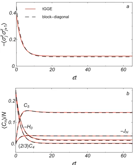
4.3 Results . . . . 88
4.4 Further experimental setups . . . . 93
4.4.1 Detection of GGEs in solids . . . . 93
4.4.2 Detection of GGEs in trapped ion systems . . . . 95
5 Generalized hydrodynamics and phase transitions in open quantum systems 101 5.1 Space-dependent Lagrange parameters . . . 103
5.1.1 Homogeneous expansion point . . . 104
5.1.2 Gradient expansion . . . 105
5.2 Transitions in weakly open spin chains . . . 107
5.2.1 Symmetric potential . . . 107
5.2.2 Asymmetric potential . . . 110
6 Stability of long range order in a driven O(3) Heisenberg chain 113 6.1 Introduction . . . 113
6.1.1 Motivation . . . 113
6.1.2 Mermin-Wagner theorem . . . 114
6.1.3 Spin wave theory in equilibrium . . . 115
6.1.4 Flocking . . . 118
6.2 Spin current and long range order . . . 119
6.2.1 The model . . . 119
6.2.2 Floquet spin wave theory . . . 121
6.2.3 Floquet-Boltzmann equation . . . 123
Contents 5
6.2.4 Classical simulation . . . 129
6.3 Field theoretical approach and stability analysis . . . 136
6.3.1 Haldane mapping . . . 136
6.3.2 Stability analysis . . . 138
7 Conclusion and Outlook 143 Bibliography 145 Appendix A Zeroth order expansion point 153 Appendix B Thermal state of the weakly open spin chain in the Ising limit 155 Appendix C Phase transitions in weakly open spin chains 157 Appendix D Equations of motion of the two continuum fields m and φ 161 Appendix E Dedication and Declaration 163 E.1 Dedication . . . 163
E.2 Declaration . . . 164
E.3 Teilpublikationen . . . 164
Zusammenfassung
Unsere Umgebung und die Natur als Ganzes betrachtet sind grundsätzlich nicht im Gleichgewicht.
Die Existenz von Leben auf der Erde ist nur aus diesem Grund möglich. Alltägliche Beispiele für Nichtgleichgewichtsprozesse sind verschiedene Wetterphänomene, die durch Luft- und Wärmeströme angetrieben werden, Staus auf Autobahnen oder das Schwarmverhalten von Tieren in Gruppen. Diese stehen exemplarisch für viele weitere Phänomene und motivieren, ein besseres Verständnis von Nicht- gleichgewichtsprozessen - seien sie klassischer oder quantenmechanischer Natur - zu entwickeln.
Im Nichtgleichgewicht sind die bekannten Konzepte für Gleichgewichtssysteme im Allgemeinen nicht oder nur approximativ anwendbar. Zu diesen Konzepten zählt, dass sich alle makroskopischen Ströme im Mittel zu Null addieren und der Gleichgewichtszustand eines Systems nur durch das fundamentale Prinzip der Entropiemaximierung und die vorliegenden Symmetrien bestimmt ist. Nach dem Noether Theorem, einer der grundlegendsten Beziehungen der Physik, ist jede kontinuierliche Symmetrie mit einer zugehörigen Erhaltungsgröße verbunden.
In dieser Arbeit betrachten wir Vielteilchen-Quantensysteme mit Erhaltungsgrößen, von denen ein Teil durch eine schwache äußere Störung verletzt wird. Wir zeigen, dass unter diesen Umständen hochgradige Nichtgleichgewichtszustände erreicht werden können, die sich durch große Ströme auszeichnen. Das Phänomen, dass eine kleine Störung einen sehr großen Effekt haben kann, falls diese Erhaltungsgrößen schwach verletzt, lässt sich zum Beispiel anhand eines Treibhauses veran- schaulichen. Im Inneren des Treibhauses ist aufgrund der guten Isolierung die Energie näherungsweise erhalten. Als Konsequenz kann das Innere sogar nur durch schwache Sonnenlichteinstrahlung auf sehr hohe Temperaturen erwärmt werden.
Die Arbeit gliedert sich wie folgt: Im ersten Kapitel führen wir analytische und numerische Methoden sowie grundlegende Konzepte ein, die in der Arbeit verwendet werden oder zum Verständnis der weiteren Ausführungen beitragen.
Im zweiten Kapitel entwickeln wir eine Störungstheorie für den stationären Zustand eines schwach
getriebenen Systems mit näherungsweisen Erhaltungsgrößen. Dabei verwenden wir als Entwick-
lungspunkt ein verallgemeinertes Gibbs Ensemble (GGE), das alle approximativen Erhaltungsgrößen
des Modells beinhaltet. Definiert ist das GGE im stationären Zustand nur durch die Form der
schwachen äußeren Störung, beziehungsweise durch das Gleichgewicht von verallgemeinerten Heiz-
und Kühlprozessen. Wir verifizieren die Gültigkeit der Störungstheorie für zwei schwach gestörte
fermionische Modelle, in denen jeweils die Teilchenzahl und die Energie approximativ erhalten sind.
2 Contents Im dritten Kapitel wenden wir unsere Theorie systematisch auf schwach getriebene integrable Sys- teme an, die eine makroskopische Anzahl von Erhaltungsgrößen besitzen, wobei wir die Analyse auf die nullte Ordnung der Störungstheorie beschränken. Wir zeigen, dass das Konzept von GGEs, gegen frühere Annahmen, auch in Anwesenheit von schwachen integrabilitätsverletzenden Störungen anwendbar ist, falls zusätzlich "in Freiheitsgrade gepumpt wird", die durch approximative Symmetrien näherungsweise beschützt sind. Weiterhin zeigen wir numerisch, dass auch die Zeitentwicklung von schwach gestörten integrablen System durch ein zeitabhängiges GGE beschrieben werden kann.
Im vierten Kapitel schlagen wir verschiedene Methoden vor, wie unsere Theorie experimentell belegt werden könnte. Insbesondere formulieren wir einen Vorschlag für effiziente Spin- und Wärmepumpen.
Im fünften Kapitel führen wir das Konzept eines GGEs mit ortsabhängigen Lagrange-Multiplikatoren ein, mit dem sich räumlich inhomogene Zustände beschreiben lassen können. Ferner stellen wir zwei konkrete Beispiele vor, wie solche Inhomogenitäten durch eine homogene Kopplung an ein Bad erzeugt werden können. Diese Formulierung erlaubt es, Phasenübergänge und spontane Symme- triebrechungen zu untersuchen.
Im letzten eigenständigen Kapitel betrachten wir ein periodisch gestörtes O(3)-symmetrisches Heisen-
berg Modell in einer Dimension, wobei die Störung derart konstruiert ist, dass sie einerseits die
Rotationssymmetrie des Modells nicht bricht, aber andererseits in Anwesenheit eines antiferromag-
netischen Ordnungsparameters einen endlichen Spinstrom induziert. Wir untersuchen, inwieweit in
einem solchen Modell ein Zustand mit langreichweitiger Ordnung stabil ist und es zur spontanen
Symmetriebrechung kommen kann.
Summary
Our environment and nature as a whole are fundamentally not in equilibrium. The existence of life on earth is only possible for this reason. Everyday examples of non-equilibrium processes are various weather phenomena driven by air and heat flows, traffic jams on motorways or the swarm behavior of animals in groups. These are just a few examples of many more phenomena and motivate a better understanding of non-equilibrium processes in classical as well as quantum systems.
Non-equilibrium means that the known concepts, which are valid in equilibrium, are generally not or only approximately applicable. In equilibrium, all macroscopic currents add on average up to zero and the configuration of a system is solely determined by the fundamental principle of entropy maximization and the symmetries present in the system. According to the Noether theorem, which represents one of the most fundamental relations in physics, each continuous symmetry is associated with a conservation law.
In this thesis, we consider quantum systems that have a set of conservation laws of which some are weakly violated by an external perturbation. We show that under these circumstances highly non-equilibrium states can be reached which are characterized by large currents. The phenomenon that a small perturbation can have a very large effect if it breaks a conservation law can, for example, be illustrated with a greenhouse. Inside the greenhouse the energy is approximately conserved due to the good insulation. As a consequence, the interior can be heated up to very high temperatures by even weak sunlight.
The work is structured as follows: In the first chapter we introduce analytical and numerical methods as well as basic concepts that are used within this thesis.
In the second chapter we develop a perturbation theory for the stationary state of weakly perturbed many-particle systems with approximate conservation laws. As an expansion point, we use a general- ized Gibbs ensemble (GGE), which includes all approximately conserved quantities of the system.
In the stationary state, the GGE is only defined by the form of the weak external perturbation or equivalently by the balance of generalized heating and cooling processes. We verify the validity of the perturbation theory for two weakly perturbed fermionic models, in which the particle number and the energy are approximately conserved.
In chapter three we apply our theory systematically to weakly driven integrable systems that have an
extensive number of conservation laws where we limit our analysis to zeroth order in perturbation
theory. We show that the concept of GGEs can, against previous assumptions, also be applied in
4 Contents the presence of weak integrability breaking perturbations if one ’additionally pumps into degrees of freedom’ that are approximately protected by symmetries. Furthermore, we provide numerical evidence that the time evolution of weakly perturbed integrable systems can be described by a time- dependent GGE. In the fourth chapter we present different suggestions of how our theory can be verified experimentally. In particular, we formulate a proposal for efficient spin and heat pumps based on approximate integrability.
In the fifth chapter, we introduce the concept of GGEs with space-dependent Lagrange parameters that can be used to describe spatially inhomogeneous states. Furthermore, we give two concrete examples of how such inhomogeneities can be generated by a homogeneous coupling to a non-thermal bath.
This formulation allows investigating phase transitions and spontaneous symmetry breaking.
In the last chapter we consider a periodically driven antiferromagnetic O(3) Heisenberg model in
one-dimension, where the perturbation is constructed in such a way that on the one hand, it does not
break the rotation symmetry of the model, and on the other hand, induces a finite spin current in the
presence of a finite antiferromagnetic order parameter. We investigate to what extent in such a model
a state with long range order is stable and spontaneous symmetry breaking can occur.
Chapter 1
Introduction
1.1 Methods
1.1.1 Density matrix formalism
The configuration of a quantum mechanical system is described by an element in a Hilbert space, the so-called quantum state. The time evolution of an abstract state |ψ(t)⟩ is governed by the Schrödinger equation
i∂
t|ψ (t)⟩ = H |ψ (t)⟩ , (1.1)
where H is the Hamiltonian of the system considered. Note that we set ¯ h and all other appearing phys- ical constants to one throughout this thesis. The formal solution of Eq. (1.1) for a time-independent Hamiltonian is given by |ψ(t)⟩ = U(t,t
0) |ψ(t
0)⟩ where U (t,t
0) := e
−iH(t−t0)denotes the time evolu- tion operator and |ψ(t
0)⟩ the initial state at t = t
0. In the case of a time-dependent Hamiltonian, the time evolution operator needs to be replaced by a time-ordered exponential U (t,t
0) = T ˆ exp(−i R
tt0
dt
′H(t
′)) where ˆ T is the time-ordering operator [1].
Of special interest are the expectation values of physical quantities, also called observables, which can, in principle, be measured in experiments. According to quantum mechanics, physical quantities are described by hermitian operators which act on the underlying Hilbert space. The expectation value of an observable O in a state |ψ(t)⟩ is given by ⟨O⟩ = ⟨ψ(t)|O|ψ (t)⟩. Using the cyclicity property of the trace this formula can be also written as
⟨O(t)⟩ = Tr [O |ψ (t)⟩ ⟨ψ (t)|] = Tr[Oρ (t)]. (1.2)
Eq. (1.2) defines the statistical operator, also called density matrix ρ (t), of a pure state |ψ (t)⟩. If
a system is in a pure state, its density matrix is simply a projection onto this state. In general, the
6 Introduction density matrix for a statistical mixture of orthonormal states {|ψ
i⟩} reads
ρ(t) = ∑
i
p
i|ψ
i(t)⟩ ⟨ψ
i(t)| , (1.3) where p
iis the probability that the system is in state |ψ
i(t)⟩. The density matrix has the following properties: ρ = ρ
†(hermicity), ρ ≥ 0 (positivity) and Tr[ρ ] = 1 (normalization). Starting from the Schrödinger equation, one can derive an equation of motion for ρ(t),
d
dt ρ(t) = L ˆ
0ρ (t), L ˆ
0ρ(t) := −i[H
0, ρ(t)] (1.4) which is referred to as Liouville-von-Neumann equation. The dynamics of ρ(t) is governed by the so-called Liouville superoperator (Liouvillian) L ˆ
0. The name superoperater origins in the fact that L ˆ
0does not act on states but on operators. While states live in a Hilbert space of dimension d, the dimension of the space of operators acting on this d-dimensional Hilbert space is d
2. In the following, we denote superoperators by letters with hats. However, we will drop the prefix super in some situations to increase readability.
In the presence of dissipation which could, for example, arise due to a coupling to an external bath, the Liouvillian can under certain assumptions be extended by an additional non-unitary superoperator (dissipator) ˆ D , L ˆ
0→ L ˆ = L ˆ
0+ D ˆ and Eq. (1.4) is then simply referred to as Liouville equation.
The formal solution of Eq. (1.4) is given by ρ(t) = e
Lˆtρ(t
0) where ρ(t
0) is the initial density matrix at time t = t
0. For a time-dependent Liouvillian the time evolution superoperator again has to be replaced by a time-ordered exponential. The eigenvalues of L ˆ are in general complex. Their real parts are less than or equal to zero if the described physical system is stable. While the imaginary parts of the eigenvalues originate in the Hamiltonian dynamics, the real parts are due to dissipation and lead to relaxation [2].
The left {|ν
α)} and right {|µ
α)} eigenvectors of L ˆ do in general not form an orthogonal set as the Liouville superoperator is not hermitian in the absence of time-reversal symmetry. The time evolution of the density matrix in terms of right eigenvectors reads
ρ(t) = ∑
α
c
αe
λα(t−t0)|µ
α), L ˆ |µ
α) = λ
α|µ
α) (1.5) and the steady state density matrix ρ
∞is defined by L ˆ ρ
∞= 0. The conservation of probability guarantees the existence of at least one steady state. The relaxation time, which is the time after which the steady state is reached, is determined by the so-called Liouvillian gap, i.e. min
α|Re(λ
α)|.
For our purpose, it is useful to introduce a projection (super)operator ˆ P onto the right eigenstates of L ˆ . In the general case of non-orthogonal eigenstates, ˆ P can be represented as
P ˆ = ∑
α,β
χ
−1α β
|µ
α)(µ
β|, χ
α β= (µ
α|µ
β) (1.6)
1.1 Methods 7 where density matrices are interpreted as vectors and (.|.) denotes the standard scalar product. The adjoint Liouville superoperator L ˆ
†can be defined through the relation Tr[O L ˆ ρ] = Tr[
L ˆ
†O ρ]. In quantum mechanics there are different representations, also referred to as different pictures, to describe the time evolution of states, observables and density matrices, respectively. In the Schrödinger picture that is used in Eq. (1.1), states evolve in time while observables are time-independent where we neglect an explicit time-dependence. In contrast to that, in the Heisenberg picture the time evolution is transferred to the operators under the constraint that expectation values do not change. The time evolution of an observable O in a state | ψ (t)⟩ is given by
⟨ψ (t)|O|ψ (t)⟩ = ⟨ψ(0)e
iHt|O|e
−iHtψ(0)⟩ = ⟨ψ(0)|e
iHtOe
−iH0t|ψ(0)⟩
= ⟨ψ(0)|O
(H)(t)|ψ (0)⟩
where we have set t
0= 0 for convenience. Hence, in the Heisenberg picture the time evolution of operators reads O
(H)(t) = e
iHtOe
−iHt. Also commonly used is the interaction picture representation in situations when the Hamiltonian can be split into a free Hamiltonian H
0and an (time-dependent) interacting part H
I(t) such that H = H
0+ H
I(t). This motivates to introduce the time evolution operators U
0(t) = exp(−iH
0t) and U
I(t) = U
0†(t)U(t). Using U
0(t) and U
I(t) the expectation value of O(t) reads
⟨ψ(t)|O|ψ (t)⟩ = ⟨ψ (0)U
†(t)|O|U(t)ψ (0)⟩
= ⟨ψ (0)U
†(t)U
0(t)|U
0†(t)OU
0(t)|U
0†(t)U(t)ψ (0)⟩
= ⟨ψ (0)U
I†(t)|U
0†(t)OU
0(t)| U
Iψ (0)⟩ .
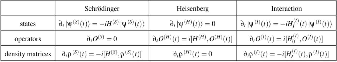
The equations of motion for states, operators and density matrices in the different pictures are summarized in table 1.1.
Schrödinger Heisenberg Interaction
states ∂t|ψ(S)(t)⟩=−iH(S)|ψ(S)(t)⟩ ∂t|ψ(H)(t)⟩=0 ∂t|ψ(I)(t)⟩=−iHI(I)(t)|ψ(I)(t)⟩
operators ∂tO(S)=0 ∂tO(H)(t) =i[H(H),O(H)(t)] ∂tO(I)(t) =i[H0(I),O(I)(t)]
density matrices ∂tρ(S)(t) =−i[H(S),ρ(S)(t)] ∂tρ(H)(t) =0 ∂tρ(I)(t) =−i[HI(I)(t),ρ(I)(t)]
Table 1.1 Time evolution of states, operators and density matrices in the Schrödinger, Heisenberg and Interaction picture.
1.1.2 Linear response theory
In this section, we give a short introduction to linear response theory based on the lecture notes of Prof. D. Tong [3].
Linear response theory deals with the response of a system to an external influence which could, for
example, be an applied electromagnetic field or a coupling to an external bath. In linear response
8 Introduction theory it is assumed that the external perturbation is small such that the response of the system can be calculated to first order in the perturbation amplitude. Then, the change of the expectation value of an observable O
idue to an external force φ
jcan be written as
δ ⟨O
i(t)⟩ = Z
dt
′∑
j
χ
i j(t,t
′)φ
j(t
′) (1.7) where χ
i jis called response function. In the following, we assume that the system considered is invariant under translations in time, hence allowing us to write χ
i j(t,t
′) = χ
i j(t − t
′). As Eq. (1.7) then becomes a convolution, its Fourier transformation factorizes
δ ⟨O
i(ω)⟩ = Z
dt
′Z
dt ∑
j
e
iωtχ
i j(t − t
′)φ
j(t
′)
= Z
dt
′Z
dt ∑
j
e
iω(t−t′)χ
i j(t −t
′)e
iωt′φ
j(t
′)
= ∑
j
χ
i j(ω)φ
j(ω).
Thus, in a linear approximation, the system responds at the same frequency ω as it is perturbed with. For simplicity, we will drop the indices i, j for the moment. Since the expectation value of an hermitian observable is real, χ(t − t
′) must be real as well. (In the general case χ must be a hermitian matrix. However, in the basis where χ is diagonal the problem can be reduced to the case considered here.) As a consequence χ
′(ω ) := Re(χ (ω )) is an even and χ
′′(ω ) := Im(χ(ω)) is an odd function of ω. Likewise, the Fourier transformation of χ
′(ω) and χ
′′(ω) are even and odd under time reversal, respectively. The imaginary part χ
′′(ω ), which is also called spectral function, therefore describes dissipative processes. It can be written in terms of χ (ω) as χ
′′(ω ) = −
2i[χ (ω ) − χ
∗(ω )].
The response function χ(t − t
′) describes how a perturbation at time t
′influences some quantity of interest at time t. As the past can not be affected by the future it directly follows that
χ(t − t
′) = 0 for t < t
′,
which is referred to as causality property. For a quantum mechanical system whose Hamiltonian H(t) = H
0+ θ (t)∆H
j(t) can be split into a dominant part H
0and a weak perturbation ∆H
j(t), the response function can be calculated as follows
⟨O
i⟩(t) = Tr h
ρ
(I)(t)O
(I)i(t) i
= Tr h
ρ
0e
iRt
0∆H(I)j (t′)dt′
O
(I)i(t)e
−iR0t∆H(I)j (t′)dt′i
≈ Tr
ρ
01 + i
Z
t 0∆H
(I)j(t
′)dt
′O
(I)i(t)
1 − i Z
t0
∆H
(I)j(t
′)dt
′≈ ⟨O
i⟩
0+ Z
∞0
χ
i j(t −t
′)dt
′,
1.1 Methods 9 where we have assumed that the system is in a thermal equilibrium state ρ
0of the unperturbed system at t < 0. Moreover, we have set ⟨.⟩
0= Tr[.ρ
0] for the corresponding expectation value. The change of the expectation value δ ⟨O
i⟩ = ⟨O
i⟩ − ⟨O
i⟩
0due to the perturbation is the integral over
χ
i j(t − t
′) := −iθ(t − t
′)⟨[O
(H)i(t),∆H
(H)j(t
′)]⟩
0. (1.8) This result is known as the Kubo formula. From the Kubo formula, we can deduce that the quantum mechanical response function can be written in terms of a two-point correlation function. In general two-point correlation functions are a measure for variances or fluctuations. On the other hand, the imaginary part of the response function encodes the amount of dissipation in a system. This implies that there is a connection between fluctuations and dissipation in quantum systems that can be formulated in terms of the so-called fluctuation-dissipation theorem (FDT). In order to find one possible formulation of the FDT we consider the correlation functions
C
i j>(t) = ⟨O
i(t)O
j(0)⟩
0, (1.9) C
i j<(t) = ⟨O
i(0)O
j(t)⟩
0and set ∆H
j= O
j. With the help of Eq. (1.9), the imaginary part of the response function can be written as
χ
i j′′(t) = − i
2 (χ
i j(t) − χ
ji(−t))
= − 1
2 (θ (t) [⟨O
i(t)O
j(0)⟩
0− ⟨O
j(0)O
i(t)⟩
0] − θ (−t) [⟨O
j(−t)O
i(0)⟩
0− ⟨O
i(0)O
j(−t)⟩
0])
= 1
2 C
<ji(t) − C
i j>(t) ,
where we have used (χ
i j(t))
∗= χ
ji(−t), θ(t)+θ(−t) = 1 and the fact that the equilibrium expectation value fulfills ⟨O
i(−t)O
j(0)⟩
0= ⟨O
i(0)O
j(t)⟩
0. Employing the cyclicity property of the trace one can show that the Fourier transformations of C
>ji(t) and C
<i j(t) are connected through
C
>ji(ω ) = e
β ωC
i j<(ω ), C
<ji(ω ) = e
−β ωC
i j<(−ω ). (1.10) With this relation, we arrive at
χ
i j′′(ω ) = − 1 2
1 − e
−β ωC
>i j(ω). (1.11)
While the left side of Eq. (1.11) quantifies the amount of dissipation in the system, the right side
captures the fluctuations C
i j>(ω ) in equilibrium. Eq. (1.10) provides an experimental tool to test
whether a piece of matter is in thermal equilibrium or not. The response of an experimentally
accessible observable could, in principle, be measured in a typical scattering experiment such as
Raman scattering at energy differences ω and −ω of the incoming and outgoing particles. If the
10 Introduction system is in equilibrium, the ratio C
ii<(−ω )/C
ii<(ω ) is equal to the Boltzmann factor e
β ω. Away from equilibrium we expect that this relation is violated.
1.1.3 Bogoliubov transformation
The Bogoliubov transformation is a method to diagonalize Hamiltonians that can be written as a sum of bilinear terms while simultaneously preserving the fermionic or bosonic commutation relations of the involved operators. The topic is treated in many textbooks. Here, we mainly follow [4]. As an example, we consider the bosonic case, which appears again later in Ch. 6, for a general Hamiltonian
H = const + ∑
k
ε
ka
†ka
k+ ε
ka
ka
†k+ γ
ka
†ka
†−k+ γ
k∗a
ka
−k= const + ∑
k
a
†ka
−kε
kγ
kγ
k∗ε
k! a
ka
†−k!
, C
k:= ε
kγ
kγ
k∗ε
k!
with ε
k2> |γ
k|
2and γ
k= γ
−k. Our aim is to find a transformation T
kthat diagonalizes H and preserves [a
k′,a
†k] = δ
k,k′as well as [a
k′,a
k] = [a
†k′,a
†k] = 0. We define Ψ
†k:= (a
†k,a
−k) and denote the new coordinates by ˜ Ψ
†k= ( a ˜
†k, a ˜
−k) such that ˜ Ψ
k= T
kΨ
kwhere T
kis given by
T
k= u
kv
kv
∗−ku
∗−k! .
The commutators [a
k′,a
†k] and [a
k′, a
k] then transform as
[ a ˜
k′, a ˜
†k] = [u
k′a
k′+ v
k′a
†−k′,u
∗ka
†k+ v
∗ka
−k] = (|u
k|
2− |v
k|
2)[a
k′, a
†k] =
!δ
kk′⇒ |u
k|
2− |v
k|
2= 1 (1.12)
[ a ˜
k′, a ˜
k] = [u
k′a
k′+ v
k′a
†−k′,u
ka
k+ v
ka
†−k] =
!0
⇒ u
−kv
k− v
−ku
k= 0. (1.13)
In order to satisfy condition Eq. (1.13) we assume that u
k= u
−kand v
k= v
−khold. Moreover, condition Eq. (1.12) is trivially fulfilled if we set
u
k= e
iφ1,kcosh(θ
k), v
k= e
iφ2,ksinh(θ
k).
1.1 Methods 11 Using relation Eq. (1.12) the inverse transformation from ˜ Ψ
kto Ψ
kreads
Ψ
k= T
k−1Ψ ˜
k= u
∗k−v
k−v
∗ku
k! Ψ ˜
kas det(T
k) = |u
k|
2− |v
k|
2= 1. The transformed Hamiltonian becomes H = ∑
k
(T
k−1Ψ ˜
k)
†C
kT
k−1Ψ ˜
k= ∑
k
Ψ ˜
†k−v
∗ku
kγ
k+ |u
k|
2ε
k− v
ku
∗kγ
k∗+ ε
k|v
k|
2u
2kγ
k+ v
2kγ
k∗− 2u
kv
kε
k(v
∗k)
2γ
k+ (u
∗k)
2γ
k∗− 2ε
kv
∗ku
∗k|v
k|
2ε
k− v
∗ku
kγ
k− v
ku
∗kγ
k∗+ |u
k|
2ε
k!
Ψ ˜
k. (1.14)
When we parameterize γ
k= |γ
k|e
iϕkby its absolute value |γ
k| and argument ϕ
k, the dependence on ϕ
kvansihes for φ
1,k= −ϕ
k/2 and φ
2,k= ϕ
k/2. To diagonalize the Hamiltonian, we define the angle θ
ksuch that the off-diagonal terms in Eq. (1.14) vanish. For the chosen values for φ
1,kand φ
2,kthe two off-diagonal terms are real and identical. This yields the condition
|γ
k|(sinh
2(θ
k) + cosh
2(θ
k)) − 2ε
kcosh(θ
k) sinh(θ
k) =
!0
⇒ tanh(2θ
k) = |γ
k| ε
k,
where we have used the identities sinh(2α ) = 2 sinh(α ) cosh(α ) and cosh(2α ) = sinh
2(α )+cosh
2(α).
With the help of the transformation T
k, we finally arrive at H = const + ∑
k
ω
ka ˜
†ka ˜
k,
ω
k= cosh
2(θ
k) + sinh
2(θ
k)
ε
k−2 cosh(θ
k) sinh(θ
k)|γ
k| = q
ε
k2− |γ
k|
2.
Alternatively, the approach outlined above can be reformulated as a pure diagonalization problem. In order to do so, we first write the constraints set by the commutation relations in terms of [Ψ
k,i,Ψ
k,j] = σ
i jzwhere σ
zdenotes the third Pauli matrix. The transformed commutation relations then read
σ
i jz= [
!Ψ ˜
k,i, Ψ ˜
†k,j] = [(T
kΨ
k)
i,(T
kΨ
k)
†j] =
T
kσ
zT
k†i j
. (1.15)
Multiplying Eq. (1.15) from the right with σ
zyields an expression for the inverse of T
k, T
k−1= σ
zT
k†σ
z. By setting ˜ T
k:= T
k−1, we obtain
H = const + ∑
k
Ψ ˜
†kT ˜
k†C
kT ˜
kΨ ˜
k= const + ∑
k
Ψ ˜
†kC ˜
kΨ ˜
k12 Introduction which suggests that ˜ T
khas to be chosen such that ˜ C
k:= T ˜
k†C
kT ˜
kis diagonal. This is equivalent to diagonalizing the matrix σ
zC
kas
σ
zC ˜
k=
σ
zT ˜
k†σ
zσ
zC
kT ˜
k= T ˜
k−1σ
zC
kT ˜
k. In general, σ
zC
kis not hermitian and the transformation ˜ T
kis not unitary.
1.2 Closed quantum systems
A quantum system is called closed if it is completely isolated from its environment. While the whole universe is expected to represent a closed system, each subsystem of it is even under the best laboratory conditions exposed to external perturbations and therefore not truly isolated. Nevertheless, in some experiments, as in ultracold atom setups, systems can on experimentally relevant timescales to a good extent be considered to be closed [5]. To this end the timescales of decoherence and dissipation have to be much longer than the timescale of the experiment. In typical ultracold atom experiments atoms are cooled down to very low temperatures up to ∼ 10
−9K and trapped in optical lattices [6]. Using these experimental setups it is possible to realize models known from condensed matter physics like the Hubbard [7] and the Heisenberg model [8], whose coupling parameters and lattice constants can to high precision be manipulated experimentally.
The Hamiltonian H
0of a closed system is time-independent and its time evolution is unitary. As a consequence energy is conserved at all times. As pointed out above, the time evolution of an initial state |ψ
0⟩ reads
|ψ (t)⟩ = e
−iH0t|ψ
0⟩ . (1.16)
The dynamics of |ψ (t)⟩ is completely deterministic. If the state |ψ(t)⟩ is known at some point in time t, the state |ψ (t
′)⟩ at any other time t
′can be deduced from Eq. (1.16). For the state |ψ (t)⟩ the expectation value of an operator O is given by
⟨O
(H)(t)⟩ = ⟨ψ
0|e
iH0tOe
−iH0t|ψ
0⟩ = ∑
n,m
c
nc
∗me
i(Em−En)tO
nm(1.17)
= ∑
n
|c
n|
2O
nn+ ∑
n̸=m
c
nc
∗mO
mne
i(Em−En)t,
where we have used the eigenstates |n⟩ ,|m⟩ and the corresponding eigenvalues E
n, E
mof H
0and
the notation O
nm:= ⟨n|O|m⟩, c
n:= ⟨n|ψ
0⟩. The first term in the second line of Eq. (1.17) is time-
independent while the second one shows oscillatory behavior. Observables that commute with H
0are
time-independent and conserved. An observable O is said to equilibrate under the dynamics of the
1.2 Closed quantum systems 13 system if the long-time limit expectation value ⟨O(t)⟩ relaxes to the time-averaged value ⟨O
(H)⟩
eq[9],
⟨O
(H)(t)⟩ −→
t→∞
⟨O
(H)⟩
eq:= lim
T→∞
1 T
Z
T 0dt⟨O
(H)(t)⟩. (1.18) In generic systems, without any symmetries, there are no degeneracies in the energy spectrum. As a consequence, the second term in Eq. (1.17) averages to zero, such that
⟨O
(H)⟩
eq= ∑
n
|c
n|
2O
nn. (1.19)
Equivalently, Eq. (1.19) can be written as ⟨O
(H)⟩
eq= Tr[Oρ
DE] where ρ
DE= ∑
n|c
n|
2|n⟩ ⟨n| is the so-called diagonal ensemble [10]. It is important to note that the second term in Eq. (1.17) only becomes exactly zero in the thermodynamic and long-time limit. For finite systems, there is always the possibility of quantum revivals, meaning that the sum of a finite number of oscillating terms can always come arbitrary close to its initial condition [11, 12]. However, in generic systems, such events happens on very long time scales and can often be neglected.
1.2.1 Integrability
Nature is far too complex to be described in an exact way. Even simplified physical models can, in general, not be solved analytically. Despite that, there is a class of models which have a particularly rich underlying structure that often allows for an analytical solution. These systems are characterized by an extensive set of constants of motion and are referred to as integrable. The existence of constants of motion enables one to determine the dynamics of the system by integration. Thus, it is not necessary to find the solution of a set of potentially coupled differential equations, but to solve a system of ordinary equations or integrals. However, that can still be a very challenging task and one might not be able to solve the system completely with the available means.
Classical dynamics is characterized by trajectories in phase space which is spanned by all possible position xxx and momentum variables p p p. The dynamics of a quantity f that is function of these phase space variables is governed by
dtdf = { f ,H} where H denotes the Hamiltonian and {A,B} :=
∑
k ∂A∂xk
∂B
∂pk
−
∂A∂pk
∂B
∂xk
the Poisson bracket. In contrast to generic systems, integrable systems do not explore the whole phase space, but are typically limited to certain orbits and often show quasiperiodic behavior in their dynamics [13]. Famous examples of classical integrable systems are the two-body Kepler problem, the classical harmonic oscillator and the Korteweg-de-Vries equation. Integrability is a very fine-tuned and fragile property. If a weak anharmonicity is introduced in the harmonic potential or a light third mass is added in the case of the two-body Kepler problem, integrability is immediately lost.
A mathematical rigorous definition of integrability can be given as follows: A classical system
described by a Hamiltonian H(q q q, p p p) with 2 f degrees of freedom is called Liouville integrable if f
functionally independent constants of motion C
iexist that commute with the Hamiltonian {C
i,H} = 0
14 Introduction and also mutually commute with each other {C
i,C
j} = 0 [14].
The Liouville-Arnold theorem states that the Hamiltonian of an integrable system can be mapped to a canonical form which does not depend explicitly on time but only on the new canonical action-angle coordinates being constant or evolving linearly in time [15]. Note that, in principle, in any classical interacting many-particle system, the starting points of all trajectories in phase space are constants of motion as they do not change with time. However, these are not constants of motion in the sense of Liouville integrability. For a given configuration of the system at time t > t
0, where t
0is the initial time, they can, in general, only be determined by solving the coupled equations of motion and then evolving the system backward in time.
It seems natural to define integrability in quantum systems by taking the classical definition and replacing the 2 f dimensional phase space by a f dimensional Hilbert space, Poisson brackets by commutators and independent functions in phase space by algebraically independent operators
[C
i,H] = 0, [ C
i,C
j] = 0 ∀i, j.
However, in this analogy it is ambiguous how the constants of motion are defined. If C
icommutes with H, any algebraic function f (C
i) commutes with H as well. Moreover, every projection operator
|n⟩ ⟨n| onto an eigenstate |n⟩ of H commutes with the Hamiltonian and the number of these projection operators is as large as the dimension of the Hilbert space. Hence, according to this definition, each quantum system would be integrable.
Importantly, not all of these constants of motion are relevant in a similar sense as not all initial conditions in a classical many-particle system are constants of motion according to the Liouville theorem. An additional criterion is needed to define integrability in quantum systems. This criterion is locality. For a discrete lattice system with translational symmetry, we can define a local conservation law C
ifulfilling [ C
i,H
0] = 0 as a translation-invariant sum of local densities c
i,j[16],
C
i=
N
∑
j=1
c
i,jwhere c
i,jhas only non-trivial support on a finite number of adjacent lattice sites, i.e. c
i,j,k= 1 for
|k − j| > n
i. The number of local conserved quantities scales linearly with the system size N and not exponentially as the size of the Hilbert space. Throughout this thesis, we refer to constants of motion also as conservation laws, conserved quantities and charges interchangeably.
Quantum integrability can be associated with the existence of an extensive set of local conserved
quantities. Another approach is to say that a quantum system is integrable if a classical limit exists in
which the corresponding classical system is integrable [17]. There are integrable lattice as well as
continuum models, for example, free [18–20] and conformal field theories [21, 22], non-linear sigma
models and non-relativistic field theories like the Lieb-Liniger model [23, 24]. Examples of quantum
integrable lattice models are the X X Z spin chain [25], the transverse Ising model [26, 27] and the
Fermi-Hubbard model [28, 29] in one-dimension.
1.2 Closed quantum systems 15 In nature, only approximately integrable systems exist because any weak integrability breaking per- turbation destroys integrability. However, as already mentioned, integrable systems can, up to good precision, be realized in ultracold atom experiments, at least on certain time scales.
Quantum integrable systems can roughly be divided into two classes. Firstly, systems in which local degrees of freedom can be mapped onto non-interacting quasiparticles using a canonical transforma- tion like a Bogoliubov transformation, or bosonization techniques. This is, for example, the case for the spin-1/2 XY and the transverse Ising model. Due to the equivalence to a single (quasi)particle picture, these systems are also called quasifree [16]. Secondly, Yang-Baxter integrable systems in which multi-particle scattering can be separated into two-particle scattering events. Such systems can be diagonalized using so-called Bethe ansatz techniques [30]. Typically, integrable quantum systems are low-dimensional and feature short range interactions. Often, the notion of quantum integrability and solvability is used interchangeably. However, there are also exceptions as reported in [31].
An effective theoretical approach to test whether a finite size system is integrable or not is to investi- gate its level statistics. While the distances of adjacent eigenvalues in integrable models are Poisson distributed, in generic systems they obey, in the presence of time reversal symmetry, the statistics of the Gaussian orthogonal ensemble (GOE) and feature level repulsion [32, 33].
Transport in integrable systems is characterized by infinite conductivities. If a current j that is protected, or at least partially protected, by conservation laws is driven by a time-dependent pertur- bation E(t), the response of the system is infinitely strong. In a linear approximation, the current and the perturbation are related through j(ω ) = σ(ω)E(ω ). The real part of the conductivity σ (ω ) in frequency space can be written as Re(σ(ω)) = σ
reg(ω ) + D(T )δ (ω) where σ
reg(ω ) denotes the regular part of σ (ω) [34, 35]. The temperature-dependent Drude weight D(T ) is a weight of the non-regular contribution at ω = 0 that is non-zero if the relaxation of currents in the long-time limit is prohibited by conservation laws. In contrast to that, in generic non-integrable systems D(T ) is zero.
According to the Mazur inequality, a lower bound for the Drude conductivity is given by D(T ) = 1
2LT lim
t→∞
⟨ j(t) j(0)⟩ ≥ 1 2LT ∑
k
⟨ j C
k⟩
2⟨C
k2⟩ (1.20)
where L denotes the system size and {C
k} is a set of orthogonal conserved quantities, ⟨C
kC
l⟩ = ⟨C
k2⟩δ
kl[36].
1.2.2 The XXZ model
Within this thesis we mainly consider the spin-1/2 X X Z model in one-dimension. The Hamiltonian of the model reads
H
X X Z= ∑
j
J 2
S
+jS
−j+1+ S
−jS
+j+1+ ∆S
zjS
zj+1(1.21)
16 Introduction where J denotes the exchange interaction and ∆ the anisotropy term. The ladder operators S
±jare defined by S
±j:=
12(σ
xj±iσ
yj) and S
zj=
12σ
zwhere σ
α(α = x,y, z) are Pauli matrices. At ∆ = J the X X Z model simplifies to the SU (2) Heisenberg model. The excitation spectrum is gapless in the regime |∆| < |J| and gapped otherwise [37].
The local conserved quantities of the model can be calculated recursively using the so-called boost operator B := −i ∑
jj h
h, where h
j= 1/2J(S
+jS
−j+1+ S
−jS
+j+1) + ∆S
zjS
zj+1is the local Hamiltonian density. The conserved quantity C
i+1of order i+1 can then be obtained with the formula C
i+1= [B,C
i] for i ≥ 2 [25]. The complexity of the charges increases with increasing order. A conserved quantity C
iof order i contains local densities that have non-trivial support on maximal i neighboring sites. The most local charges of the X X Z model are the total spin in z-direction C
1= S
z, the Hamiltonian itself C
2= H
X X Zand the heat current operator
C
3= J
h= J
2∑
j
S
′j× S
′′j+1× S
′j+2, (1.22)
where we have defined S
′αj= √
λ
αS
αj, S
′′αj= p
λ
z/λ
αS
αjfor λ
z= ∆/J, λ
x= λ
y= 1. The set of local conservation laws can be divided into the sets of even {C
2n} and odd {C
2n+1} charges. Odd conservation laws are conserved currents. In contrast to the set of even charges, they are, for example, odd under time reversal and certain spatial reflection symmetries.
Due to the conservation of the heat current, the corresponding Drude weight is finite at all finite temperatures [38]. In contrast to that, the spin current operator
J
s= J ∑
j
S
xjS
yj+1− S
yjS
xj+1(1.23) is not conserved, [H
0,J
s] ̸= 0. As J
sis odd under spin-reversal while all local conservation laws of the X X Z are even under this transformation, one would expect that the spin Drude weight (also called spin stiffness) is zero. However, it was found that the Drude weight of the spin current is non-zero for
|∆| < |J| [39] which was explained recently by the detection of an additional set of charges [40, 41].
Importantly, these charges cannot be written as a sum of local densities. The corresponding charge densities can rather be considered as quasilocal, meaning that they are local up to exponential tails. In contrast to the local conservation laws, they do not exhibit spin-reversal invariance and have a finite overlap with the spin current at |∆| < |J|. Among the known quasilocal conservation laws are the families of X and Z charges [16] where the more exotic charges of the Z family even break the U(1) symmetry of the underlying model.
Due to a finite overlap between the spin current and the quasilocal charges at |∆| < |J|, the spin stiffness is non-zero indicating ballistic transport. Using the set of common eigenstates {|n⟩} of the local conservation laws the conserved part of the spin current can be constructed as
J
sc= ∑
n
⟨n|J
s|n⟩ |n⟩ ⟨n|. (1.24)
1.2 Closed quantum systems 17 1.2.3 Thermalization
One of the major hallmarks of equilibrium statistical physics is the fact that macroscopic systems with many degrees of freedom can be described by only a few parameters like, for example, temperature T and chemical potential µ. Such a coarse-grained description cannot capture all possible microscopical configurations but it can predict the typical behavior of a system on macroscopic scales. Generally, one is not interested in the position and velocities of all molecules in a classical gas or the exact wave function of a quantum many-body system but rather in measurable correlation functions and local observables. The expectation values of these observables, like energy and particle number, define macroscopic states that are compatible with many microstates. The approach of statistical physics is to replace the description of deterministically evolving microstates by a stochastic theory for macrostates.
The existence of stationary equilibrium probability distributions, also called ensembles, originates in the second law of thermodynamics, which states that the entropy increases in (almost) all processes [42, 43]. The thermal equilibrium distribution is then distinguished as the distribution with maximal entropy.
The entropy of a macroscopic state is a measure for the number of microstates that can realize the former. Thus, in equilibrium where by definition each state in configuration space is equally often reached during the time evolution, a closed system tends to be most likely in the macrostates being consistent with the most microstates. As an illustration, we consider a gas of N particles in an isolated box that is virtually divided into two halves (This is a very commonly used example. A similar setup was, for example, also considered in [44]). We assume that all particles are initialized in the left half of the box at time t = 0. After a certain equilibration time, the particles fill the whole box uniformly, as this is the macrostate with the most microscopical realizations. The entropy of a macrostate with N
1particles on the left and N − N
1particles on the right side is
S(N
1) = ln
N N − N
1= ln
N!
N
1!(N − N
1)!
≈ ln
" √
2π N
NeNp 4π
2N
1(N − N
1)
Ne1N1 N−N1 e N−N1#
= const − 1
2 (ln [N
1] + ln [N − N
1]) − N
1(ln [N
1] − 1) − (N − N
1) (ln [N − N
1] − 1) , where we have used the Stirling formula n! ≈ √
2πn (n/e)
nwhich is valid for n ≫ 1. The entropy is maximal at N
1= N/2 as
∂ S(N
1)
∂ N
1N1=N/2
=
1
2(N − N
1) − 1 2N
1+ ln [N − N
1] − ln[N
1]
N1=N/2= 0,
∂
2S(N
1)
∂
2N
1N1=N/2
= 4
1 − N N
2< 0.
Hence, in the most likely configuration half of the particles are on the left and the other half on the
right side. However, due to fluctuations on the microscopic level there is a chance to measure a
18 Introduction slightly different number of particles. The probability to find N/2 − M particles in one and N/2 + M particles in the other subsystem is
P
M= 1 2
NN N/2 ± M
≈ 1 p
π2
N e
−2M2
N
, (M ≪ N),
where 2
Nis the total number of macrostates. Fluctuations are Gaussian distributed with variance σ
2= N/4. We see that the probability for all particles N being again in the left half of the box is exponentially small in N. The second law of thermodynamics sets a fixed arrow of time towards the equilibrium state. This is referred to as irreversibility. The system can go back to its initial low-entropy configuration but the probability for this process is extremely tiny in a macroscopic system.
In the context of thermal equilibrium, it is important to introduce the concept of a thermal bath. A bath is a large thermodynamic system with so many degrees of freedom that its temperature, chemical potential, . . . do not change when it is coupled to the actual system of interest. On the contrary, it dictates the intensive parameters of the system and fixes the expectation values of the corresponding extensive quantities. It can serve as an infinite reservoir for heat, particles or other quantities that are conserved in the whole system.
To find the equilibrium distribution for a given bath coupling one can, for example, use an approach from information theory. The Shannon entropy of a discrete probability distribution is defined as [45]
S[{p
j}] = −
N
∑
j=1p
jln(p
j). (1.25)
where p
jis the probability of the system to be in a macrostate labeled by j. We aim to find the probability distribution that maximizes Eq. (1.25) in the presence of possible constraints set by a coupling to an external bath which can be incorporated in terms of Lagrange multipliers. In the case of a closed system, the only constraint is the normalization of the distribution, i.e. ∑
jp
j= 1 and the entropy is maximized by a uniform distribution with p
j= 1/N. In physics, this is referred to as the microcanonical ensemble. If the system is coupled to a heat bath that fixes the expectation value of the energy E = ∑
jp
jE
j, the Shannon entropy is maximal for
p
j(E) = 1
Z(E) e
−βEj, Z(E) = ∑
j
e
−βEj,
where β = 1/E is the inverse temperature and Z(E ) the canonical partition sum. This is the so-called
canonical ensemble. In the case of energy and particle number fluctuations one obtains the grand
canonical ensemble. These are the most commonly used ensembles in statistical physics. In the
thermodynamic limit, when the relative fluctuations of energy and particle number tend to zero (by
virtue of the central limit theorem), these ensembles are believed to be equivalent. This has been
rigorously proven for systems with short range interactions [46].
1.2 Closed quantum systems 19 Systems in equilibrium are considered to be ergodic [47]. Ergodicity means that the whole phase space is filled equally during the time evolution. As a consequence, the time average of physical observables becomes equivalent to the ensemble average which allows us to work only with time-independent probability distributions in equilibrium statistical physics. For a system in equilibrium with N discrete states, ergodicity means that all transition rates Γ
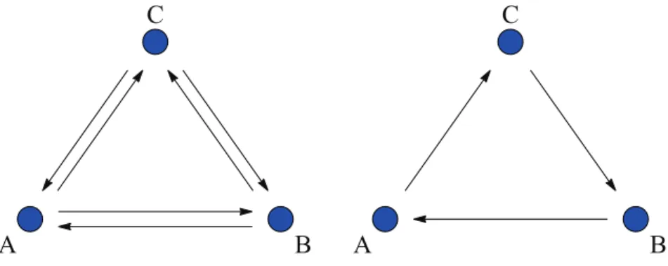
i→jbetween states i and j are non-zero and therefore all states can be reached during the dynamics. In equilibrium, the detailed balance relation
Γ
i→jP
i= Γ
j→iP
j(1.26)
holds, which implies that all probability currents vanish. This can be seen as a defining property of thermal equilibrium. Besides ergodicity, thermalization is associated with the concept of dynamical chaos [48]. A system is said to be chaotic if its final state, which is reached after some time t, is extremely sensitive to the initial conditions. Even small changes in the starting configuration can lead to a very different final state. The microscopic state of a system in equilibrium might look completely different for slightly different initial conditions. However, at macroscopic scales, the system can in both cases be well described by an equilibrium ensemble.
1.2.4 Thermalization in quantum systems
A natural question to ask is under which circumstances equilibrated observables in isolated quantum systems can be described by ensembles known from statistical physics. A typical experimental as well as theoretical approach to investigate this question are so-called quantum quenches. In a quantum quench, a system is, typically, first prepared in an eigenstate (mostly the ground state) of a Hamiltonian H(λ ). Then one parameter λ of the initial Hamiltonian is suddenly set to a new value λ
′. As a consequence, the initial state is, in general, no eigenstate of H(λ
′) anymore and evolves unitarily under the new Hamiltonian.
In the case of a generic system, the expectation value ⟨O⟩ of an observable O is expected to be given by Eq. (1.18) in the long-time limit which can also be formulated in terms of the diagonal ensemble
ρ
DE= ∑
n
|c
n|
2|n⟩ ⟨n| (1.27)
as ⟨O⟩ = Tr[Oρ
DE]. It can be said that an observable O thermalizes if its long-time limit expectation value can be reproduced by an equilibrium density matrix ρ
eqdepending only on a few parameters T, µ , . . .,
⟨O⟩ = Tr[O ρ
DE] = Tr[O ρ
eq(T,µ , . . . )]. (1.28)
Note that this statement can only be exactly true in the thermodynamic limit. It is again a priori not
clear why closed quantum systems should thermalize as their dynamics is completely unitary. This
apparent contradiction is in some sense similar to the paradox of thermalization in deterministically
20 Introduction evolving classical systems. In classical statistical mechanics the contradiction can be resolved by the assumption of ergodicity and dynamical chaos.
The question is how thermalization can be explained in quantum mechanics. A thermal state is completely independent of the initial configuration. In contrast to that, in a closed quantum system, the information about the initial conditions remains available for all times. However, it is important to note that information propagates during the time evolution and is after a sufficiently long time only accessible by global measurements. Typically, the speed at which information spreads in quantum systems is limited by the so-called Lieb-Robinson bound [49] whose explicit value depends on the details of the system. As most of the relevant physical observables are described by local operators, the information about the initial state is effectively lost as long as local measurements are concerned and ρ
DEin Eq. (1.28) might be replaced by an equilibrium distribution. Another way of defining thermalization is the following: An infinitely large system B is considered to be thermal if the reduced density matrix of all possible finite subsystems A ⊂ B is given by a thermal distribution, i.e.
ρ
A= Tr
B/A[ρ] = ρ
eq(T, µ, . . . ). (1.29) If this condition is met, it is said that the system serves as its own heat bath. A commonly used explanation to illustrate thermalization in quantum systems is the so-called Eigenstate Thermalization Hypothesis (ETH) [50, 51] which is based on two major assumptions: 1) The diagonal matrix elements O
nn= O(E
n) of an operator O depend smoothly on the energy and 2) the off-diagonal matrix elements are much smaller than the diagonal ones O
nn≫ O
nm. If we assume that all relevant energies lie within a shell of width ∆E centered around the energy E, we obtain for the expectation value of O in the long-time limit
⟨O(t)⟩ −→
t→∞
∑
n
|c
n|
2O
nn+ ∑
n̸=m
c
∗mc
ne
i(Em−En)tO
mn1),2)
≈ ∑
n,|E−En|<∆E
|c
n|
2O(E
n) ≈ 1
Ω
∆E(E) ∑
n,|E−En|<∆E