Coupled Evolution Equations for Immersions of Closed Manifolds and Vector Fields

Coupled Evolution Equations for Immersions of Closed Manifolds

and Vector Fields

Dissertation zur Erlangung des Doktorgrades der Naturwissenschaften (Dr. rer. nat.)

der Fakultät für Mathematik der Universität Regensburg

vorgelegt von

Christopher Brand

aus Regensburg

im Jahr 2018

Promotionsgesuch eingereicht am: 05. Dezember 2018

Die Arbeit wurde angeleitet von: Prof. Dr. Georg Dolzmann (Universität Regensburg)

Prüfungsausschuss: Vorsitzender: Prof. Dr. Stefan Friedl

Gutachter: Prof. Dr. Georg Dolzmann

Gutachter: Prof. Dr. Harald Garcke

weitere Prüfer: Prof. Dr. Helmut Abels

Zusammenfassung

Eine mögliche Beschreibung der elastischen Energie einer Biomembran ist durch den L ² -Abstand der mittleren Krümmung von einer spontanen Krümmung plus einer topologischen Konstante gegeben. Ein solches Energiefunktional wird oft als Helfrich Energie bezeichnet.

Wir untersuchen eine Erweiterung dieser Modellierung, bei der die spontane Krümmung durch die Oberflächendivergenz eines Vektorfeldes entlang der Fläche gegeben ist. Eine abstrakte Formulierung für Immersionen von Mannigfaltigkeiten beliebiger Dimension wird hergeleitet.

Für Kurven in der euklidischen Ebene zeigen wir für dieses Funktional Existenz von globalen Minimierern und Regularität von stationären Punkten unter den verschiedenen Nebenbedingun- gen. Mögliche Nebenbedingungen sind die Länge der Kurve, der von der Kurve eingeschlossenen Flächeninhalt und der Bildbereich des Vektorfeldes.

Außerdem leiten wir für Immersionen von Mannigfaltigkeiten beliebiger Raumdimension eine Gradientenflussdynamik her, die auf ein gekoppeltes System partieller Differentialgleichungen führt. Für dieses gekoppelte System zeigen wir lokale Wohlgestelltheit auch im Fall, dass der Fluss die Nebenbedingungen erhält.

Weiterhin zeigen wir für das uneingeschränkte Funktional sowie unter Berücksichtigung der Nebenbedingungen eine Łojasiewicz-Simon Gradientenungleichung, aus welcher man dann Rückschlüsse auf das asymptotische Verhalten des Flusses nahe lokaler Minimierer ziehen kann.

Für Kurven und Vektorfelder in der Ebene geben wir eine geometrische Größe an, deren

Kleinheit Glattheit des Flusses garantiert. Durch Reskalieren erreichen wir, dass es bereits

ausreicht, dass diese Größe endlich ist, um Singularitäten auszuschließen.

Abstract

A possible description of the elastic energy of a biological membrane is given by the L ² -distance of its mean curvature from a spontaneous curvature plus a topological constant. Such energy functional is often referred to as Helfrich energy.

We study a generalization of this model, where the spontaneous curvature arises as the divergence of a vector field along the surface. An abstract formulation for immersions of manifolds of arbitrary dimension is derived.

For plane curves we prove for this energy functional the existence of global minimizers and regularity of stationary points subject to different constraints. The constraints we considered are the length and enclosed signed area of the curve and the range of the vector field.

Furthermore, we derive a gradient-flow equation in the general situation of immersions of manifolds of arbitrary space dimension which leads to a coupled system of partial differential equations. For this coupled system we show local well-posedness even for a constraint preserving adaption of the flow.

Moreover, we show a Łojasiewicz-Simon gradient inequality for the unrestricted functional as well as in the presence of constraints. From this we draw conclusions about the asymptotic behavior of the flow close to a local minimizer.

For curves and vector fields in the euclidean plane we introduce a geometric quantity whose

smallness guarantees smoothness of the flow. By a rescaling argument we achieve that even

finiteness of this quantity suffices to exclude the formation of singularities.

Contents

Introduction 1

1 Notation and Prerequisites 11

1.1 Analysis . . . . 11

1.2 Basic Properties of Riemannian Manifolds and Hypersurfaces . . . . 11

1.3 Plane Curves . . . 13

1.4 Function Spaces on Manifolds . . . 14

1.5 Moving Hypersurfaces . . . 15

1.6 Multiplication and Composition in Sobolev Spaces . . . 20

1.7 Spaces for Parabolic Problems . . . 26

2 Curves and Vector Fields—an Anisotropic Approach 31 2.1 Vector Field in the Background . . . . 31

2.2 Vector Field on the Curve . . . 33

3 A Helfrich-Type Model for Biomembranes 39 3.1 Scaling Properties . . . 40

3.2 An Adaption of the Energy for Curves . . . 40

3.2.1 Existence of minimizers . . . . 41

3.2.2 Regularity of stationary points . . . 42

3.3 The L ² -Gradient Flow . . . . 47

3.4 The Projected L ² -Gradient Flow . . . 50

3.5 Analysis of Some Special Cases . . . . 51

4 Short-Time Existence for the Generalized Helfrich Flow 55 4.1 The Evolution Equation for the Height Function . . . 55

4.2 The Linearized Problem . . . . 57

4.2.1 Weak solutions . . . 58

4.2.2 Regularity . . . 63

4.3 The Full Equation . . . . 67

4.4 Some Non-Local Constraints . . . 72

4.5 The Unit-Length Constraint for n . . . . 77

4.6 The Parameter Trick and Implications of Maximal Regularity . . . 80

4.7 Some Useful A Priori Estimates . . . 83

5 Long-Time Behavior for Solutions of the Gradient-Flow Equation 87 5.1 A Criterion Granting Global Existence for the Flow of Curves . . . . 87

5.2 A Łojasiewicz-Simon Inequality in the Unconstrained Case . . . 98

5.3 A Łojasiewicz-Simon Inequality in the Presence of Constraints . . . 104

5.4 Stability of Minimizers . . . 111

A Numerical Experiments 115

Introduction

With the range of applications reaching from deep questions of topology and geometry to models for complex physical processes and even image segmentation, geometric evolution equations form a common basis of an extremely wide range of mathematical research areas.

Intrinsic geometric evolutions deform the metric of a Riemannian manifold in a smooth way, without consideration of any embedding or immersion. Their most prominent instance is by all accounts the Ricci flow, profoundly investigated by Hamilton. It was central in Perelman’s proof of Thurston’s geometrization conjecture, which implies the Poincaré conjecture, and the proof of the differentiable sphere theorem by Brendle and Schoen after 30 years of intensive research (cf. [11, 45, 74, 75, 86]).

Extrinsic evolutions smoothly vary mappings or immersions of a smooth manifold according to a law involving geometric quantities of this immersion. A large variety of different flows of this kind has been studied, including the harmonic-map heatflow, the Willmore flow and the mean-curvature flow, the latter being the most famous example of a whole range of curvature flows. Some of them have been introduced to improve the understanding of existence and properties of solutions of stationary geometric problems, while others are part of models for physical mechanisms, for example for phase transitions or biological membranes.

Roughly summarized, the setting of extrinsic geometric flows can be summarized as follows.

The word flow usually refers to a semi-group action. In analysis, a (local) flow is usually given implicitly through an initial value problem. The actual flow is then the mapping that relates an element x of a set—a subset of a euclidean space or some function space—to a solution of the initial value problem, given for example by an ordinary or partial differential equation, for the initial datum x. In this context, local means that the admissible parameter set—that commonly is referred to as the time variable—depends on the element in question.

This concept generalizes to the setting of two Riemannian manifolds. When (M, g) is a smooth closed and orientable Riemannian manifold of dimension d ∈ N and (N, g) is another ¯ smooth Riemannian manifold of dimension k ∈ N , then a geometric flow takes an initial map ϕ 0 : M → N and time t 0 and maps it to a solution (ϕ, T ) ∈ {M × [t 0 , t 0 + T ) → N } × (0, ∞] of an initial value problem of the form

∂ t ψ(p, t) = F (p, t, ψ(p, t), ∇ψ(p, t), . . . , ∇ ^m ψ(p, t)) on M × [t 0 , t 0 + T ) and

ψ(p, t ₀ ) = ϕ ₀ (p) on M, (1)

where F is a smooth function that takes for all p ∈ M values in T _ψ(p) N , and m ∈ N is called the order of the equation. Observe that, in this context, the time of existence of the solution, if a solution exists at all, is also to be determined. If T = ∞, the solution is called a global solution.

This generic form of a partial differential equation also includes cases that are not well-posed

in the sense of Hadamard, i.e. that an initial value problem should have a unique solution that

depends continuously on the initial value. A specific class of equations that are well-behaved in

this sense are parabolic equations. Note that there is a whole range of notions of parabolicity

INTRODUCTION

(cf. [32, Chapter 7] and [77, Chapter 6]), the archetypical example being the heat equation. The heat equation can also be seen as the flow in the direction of steepest descent, or gradient flow, of the Dirichlet energy for functions u : R ^d ⊃ Ω → R reading

E _D (u) = Z

Ω

|Du| ² dx.

Here, the gradient of E D has to be taken with respect to the usual L ² scalar product. The concept of L ² -gradient flows is also central for many geometric flows. However, the scalar-product that is used to identify the gradient may vary with the immersion, much as in Riemannian geometry.

For every geometric flow—as in general for initial value problems—one is mainly interested in the following questions.

• In what setting is the problem well-posed?

• What are possible obstructions to the existence of global solutions, i.e. singularities?

• Can these singularities be characterized and possibly overcome by a different notion of solution?

• Can we determine the asymptotic behavior of global solutions as t tends to ∞?

The answer to the first and last question can be often treated by reformulating the problem to a strictly parabolic evolution equation and adaption of special techniques from their theory.

We will follow this general approach for a specific geometric evolution equation also in this work, as will be discussed later. Also the second and fourth question will be treated in this thesis for a particular problem. With their introduction to the field of geometric evolutions often attributed to Hamilton, typical techniques include integral and interpolation estimates, maximum principles, and monotonicity formulae and constitute the heart of a large share of theorems in geometric analysis. The third question requires techniques, that are different from those used in this work. Overcoming of singularities without losing track of topological changes or uniqueness of solutions led to famous theorems (see e.g. [74], [51]).

A large class of flows is also geometric in the more specific sense that the evolution is only defined for immersions and is invariant under reparametrization of the manifold M . With the exception of the harmonic-map heat flow, this is the case for all above-mentioned flows. Let us now take a closer look on some specific evolution equations.

The mean-curvature flow arises for k > d when we define for immersions ϕ : M → N the map F in (1) to be given by F = − →

H , where − →

H is the mean curvature vector at ϕ(p, t) of the submanifold given by ϕ(·, t) around ϕ(p, t). It was suggested in the 1950s as a model for the motion of interfaces in soap froth by von Neumann [89], and for the motion of grain boundaries in an annealed, recrystallized metal by Mullins [71], who also formulated it as a partial differential equation for closed curves in the plane and found some self-similar and a translating solution, often called the grim reaper.

For compact surfaces the mean-curvature flow decreases the area of the given surface as fast as possible. When the manifold M is immersed into N by an immersion ϕ, we pull back the metric of N and obtain a surface measure dµ _ϕ . The area functional A is then simply

A(ϕ) = Z

M

1 dµ ϕ .

Comparison with the flow of a round sphere shows that any solution with compact initial datum

can only exist for finite time. Most results consider the case where N = R ^d+1 .

INTRODUCTION

For the case of the mean curvature flow of closed curves in R ² , often referred to as the curve shortening flow, Gage, Hamilton and Grayson were able to show that any embedded curve will first become convex [42] and then asymptotically round while shrinking to a point in finite time, that is proportional to the initially enclosed area [35, 36, 38].

Independently, for convex d ≥ 2 and d-dimensional hypersurfaces in R ^d+1 Huisken showed that solutions also become asymptotically round, before they disappear in a single point [48]. Relaxing the condition of convexity to mean-convexity of the initial surface, Huisken and Sinestrari [51]

described a surgery procedure, that allows one to extend the flow beyond singularities, by cutting out the parts of highest curvature, which turn out to be cylindrical, while controlling the topology. This led to a topological classification result for two-convex hypersurfaces.

Of course, over a timespan of more than 30 years, a great number of authors has contributed new results and new proofs. Therefore, for further reading on the subject we refer to introductory works of Mantegazza [68] and Colding and Minicozzi [17] and the references therein.

The Willmore flow is the flow of immersions along the steepest descent of the Willmore functional W [93], that was originally introduced for immersion of a 2-dimensional surface M in R ³ . For ϕ : M → R ³ it is given by

W (ϕ) = 1 2π

Z

M

|H| ² dµ _ϕ ,

with the mean curvature H of ϕ(M ). Willmore was in particular interested in the infimum of W among all possible immersions of surfaces of a fixed genus. The normalization factor is in the literature mostly chosen according to the preferences of the respective author.

A study of the actual flow was initiated by Kuwert and Schätzle [56]. Denoting the Laplace Beltrami operator, the second fundamental form and the choice of unit normal by ∆, A, ν, respectively, the evolution law reads

∂ _t ϕ = 1

π ∆H + H |A| ² − 1 2 H ³

ν.

Kuwert and Schätzle gave a lower bound for the time of smooth existence of the flow in terms of the initial spatial concentration of |A 0 | ² , where A 0 denotes the trace-free second fundamental form. In two subsequent papers [55, 57], they proved for any codimension that if M is a sphere and initially R

M |A 0 | ² dµ ϕ < 16π,then the flow exists for all times and converges to a round sphere. Moreover, they established a results on the structure of point singularities.

While Willmore was interested in topological invariants, for a regular curve γ in the plane with curvature κ, parametrized over a real interval I, the one dimensional analogue of Willmore’s functional, namely the quantity

Z

I

κ ² ds, (2)

was already discussed by Daniel Bernoulli and Euler [31] as an important quantity while aiming to determine the shape of an elastic rod whose endpoints are fixed, but that can move freely otherwise. This question is known as the problem of the elastica and the quantity (2) is—as we will see—still an object of mathematical research. The report on the history of elasticae by Levien [61] is a nice overview and includes historical drawings of Euler and Bernoulli of astonishing precision.

The study of elastic properties of lipid bilayers [47] led Helfrich to a model for the elastic energy of biological membranes. When the shape of the membrane is represented by an embedding ϕ of a 2-dimensional closed manifold M to R ³ , its elastic energy is described by

E(ϕ) = Z

M

1

2 k c (H − c 0 ) ² + ¯ k c K dµ, (3)

3

INTRODUCTION

where K is the Gauß curvature of the embedded surface, k c and ¯ k c are the relevant curvature- elastic moduli and c 0 is called spontaneous curvature and was originally introduced to allow for chemically different sides of the bilayer. By the Gauß-Bonnet Theorem, the quantity R

K dµ is a topological invariant and does not change, when ϕ varies continuously, that is in particular in one topological class. Considering the flow in direction of the steepest descent for E, one obtains an evolution law that is in highest order the same as that for of the Willmore flow.

However, the spontaneous curvature breaks the scaling symmetry of the energy. For immersions of 2-dimensional manifolds this flow has been analytically studied by several authors [54, 65, 72].

The one-dimensional analogue, that is the gradient flow of (2), is often called the elastic flow and has also been subject to recent investigations. For closed curves, even in arbitrary co-dimension, the behavior of this flow is now well-understood. Dziuk, Kuwert and Schätzle [28]

proved global existence and convergence (up to subsequence) to a stationary point of (2), that is an elastica.

The harmonic-map heat flow is of different nature, as it is not only depending on the shape of the immersed manifold, but also takes the particular parametrization into account. It was introduced by Eells and Sampson [29] in order to find stationary points of a generalized Dirichlet energy. For a closed, smooth Riemannian manifold (M, g) and another smooth Riemannian manifold (N, h) the energy of a smooth map u : M → N is given by

E(u) = Z

M

|du| ² dµ _g .

In their work Eells and Sampson provide conditions on intrinsic curvature quantities of N under which the flow converges indeed to a stationary point of E, called a harmonic map, independent of the initial datum. Therefore, they concluded that under such suitable assumptions on N , every smooth map from M to N is homotopic to a harmonic map. For an introduction to the theory of harmonic maps and their heat flow we refer to the book of Lin and Wang [63] who also provide a great many useful references.

An augmentation of the usual setting of extrinsic geometric flows is the abandonment of symmetries. Studying the evolution of immersions into a (non-flat) Riemannian manifold is a first step in this direction. Interesting questions emerge when the target manifold has non-trivial topology. For the curve-shortening flow, Grayson solved the case of curves in general 2-dimensional manifolds [43]. Huisken studied the mean-curvature flow of convex immersions of higher dimensional manifolds [49]. To find suitable surgery procedures is subject of very recent research [9, 10]. The Willmore energy of immersions into spheres was considered by White [92]

showing that stationary points are preserved under stereographic projection. Lamm, Metzger and Schulze [58] and Jachan [53] considered the Willmore energy and flow in manifolds that are asymptotically Schwarzschild.

A further generalization is the concept of anisotropic flows. The Russian material scientist Wulff [94] had, already at the beginning of the 20th century, evidence that the energy of the boundary of a crystalline material depends on the direction of the surface normal to the lattice structure of the crystal. He also gave a method how to determine the shape of minimal energy for a given direction dependent energy density.

Models for interfaces often incorporate directional dependence of the surface energy density.

Such energies can be described by a positive, 1-homogenous function η : R ⁿ → R . For a smooth immersion ϕ : M → R ^d+1 with a unit normal ν the energy is then defined as

E(ϕ) = Z

M

η(ν) dµ ϕ .

Analogously to the mean curvature flow, the gradient flow of anisotropic energies has been

INTRODUCTION

subject of mathematical research since the 1970s. Taylor [82] distinguished between the case of smooth and crystalline surface energies. The latter ones, arising from non convex anisotropies η, lead to polyhedral minimizing surfaces. In the case that η is strictly convex and smooth, also the minimizing shape, often referred to as the Wulff shape, is convex and smooth.

Ambient vector fields in R ^d+1 were taken into account by Wheeler [91]. For d ∈ N , curves γ : S ¹ → R ^d+1 , a vector field c : R ^d+1 → R ^d+1 and a function f : R ^d+1 → R he generalized the Helfrich energy (3) for curves by establishing the spontaneous curvature

c 0 = c ◦ γ + (f ◦ γ)τ,

where τ is the unit tangent to γ. After a short discussion of general properties of this energy, he proves that under suitable assumptions on c and f the gradient flow equation has a global solution for all initial curves and that there is a sequence of times t j → ∞ such that the curves γ(t j ) converge to a stationary point of the energy after suitable translation and reparametrization.

In Chapter 2 of this work we will discuss, how the idea of an ambient vector field can be used to construct an anisotropic and homogeneous energy for curves in the plane, and review existing literature to ascertain existence of global solutions and their asymptotic behavior.

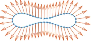
A different generalization of the Helfrich energy (3) is proposed by Bartels, Dolzmann, Nochetto and Raisch [7]. They trace back the spontaneous curvature term to the local orientation of the rod-shaped lipid molecules. This is modeled for two-dimensional membranes by the introduction of a vector field n : M → R ³ . With a physical constant δ ∈ R the quantity

δ div n

is then interpreted as the spontaneous curvature. Here div is the divergence with respect to the metric on M that is induced by the immersion ϕ : M → R ³ that represents the membrane. This situation is depicted in Figure 1 for a curve and vector field in R ² . The energy for the whole system also takes into account molecular forces between the lipid molecules and is given by

E(ϕ, n) = 1 2

Z

M

(div ϕ ν ϕ − δ div ϕ n) ² dµ ϕ + λ 2 Z

M

|∇ ϕ n| ² dµ ϕ , (4) with another physical constant λ > 0. In their work, the L ² -gradient flow of this energy is derived which leads to a system of coupled partial differential equations. Moreover, they derive a parametric finite elements scheme and present some numerical experiments.

The equation for the evolution of the immersion shares some structure with the Willmore flow. Indeed, when δ = λ = 0 the flows coincide. But for λ positive while δ = 0 the equations are coupled.

The evolution of the vector field n is governed by a law that shares its leading term with the harmonic map heat flow. This relation is of additional importance, when a supplementary length condition for n is imposed. Since ϕ represents a biological membrane, it is reasonable to assume that the area of the represented surface and its enclosed volume are constant during the evolution.

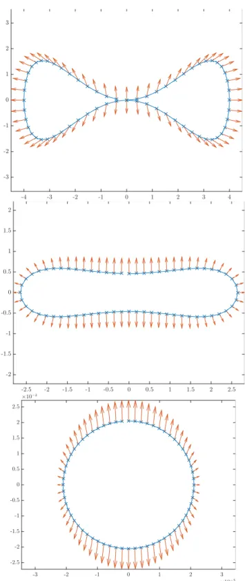
Figure 1: A plane curve with an attached vector field.

5

INTRODUCTION

The main topic of this thesis is the evaluation of the analytical properties of this generalized Helfrich energy in combinations with the above-mentioned constraints

Fixed signed volume enclosed by ϕ(M ):

Fixed surface area of ϕ(M ):

Length constraint for n:

Z

M

ϕ · ν _ϕ dµ _ϕ = V ₀ , Z

M

1 dµ _ϕ = A ₀ ,

∀ _p∈M kn(p)k _R

= 1,

(5)

for suitable choices of A ₀ and V ₀ especially not violating the isoperimetric inequality.

Considering (4) for curves and vector fields with values in R ² , inspired by arguments of [19,20], we show existence and smoothness of minimizers of the energy (4) when a length penalization term is added using variational techniques and elliptic regularity theory.

Theorem 1

For δ ≥ 0, λ > 0 the energy E given by E(γ, n) =

Z

γ

1

2 (κ + δ div(n)) ² + λ

2 |∂ s n| ² + 1 ds

has a smooth global minimizer. Furthermore, a global minimizer exists for any combination of the constraints in (5) imposed.

For a closed orientable manifold of dimension d, we consider the gradient flow of the energy (4) as derived by [7] for an immersion and a vector field with values in R ^d+1 . Due to the strong coupling of the evolution equations and due to the fact that one of them is of fourth, the other of second order, even the well-posedness of the evolution equation is not covered by standard theory. We use energy methods to solve the corresponding linearized problem and employ a typical parabolic approach to obtain a short-time existence result for initial data in a Sobolev space of sufficient regularity.

Theorem 2

For d ∈ N let M be a closed d-dimensional smooth orientable manifold. Let k > d/2 + 3 be a natural number, ϕ ₀ ∈ H ^k (M, R ^d+1 ) be an immersion and n ₀ ∈ H ^k (M, R ^d+1 ) be a vector field with kn ₀ k _R

≡ 1.

Then, there is a T > 0, such that the area and volume preserving gradient-flow equation of the energy (4) has a unique solution (ϕ, n) on M × [0, T ) and knk _R

≡ 1. Moreover, for

positive times the surface and the vector field are smooth in space and time.

The result remains valid, if we impose at most two of the three constraints in (5). If the unit-length constraint is disregarded, the condition on n 0 is obsolete.

For the questions concerning the development of singularities and the asymptotic properties

of the flow we provide first partial answers. In view of the very tame behavior of the elastic

flow and the harmonic map heat flow for curves, that both admit global solutions and converge

to stationary points, one might expect that a similar result can be established for the coupled

flow. However, the coupling terms make the situation rather involved. Using interpolation

and Sobolev inequalities we find a geometric quantity that cannot remain bounded, when a

singularity occurs.

INTRODUCTION

Theorem 3

Let (γ, n) : S ¹ × [0, T ) → R ² × R ² be a smooth gradient flow of the energy (4), that cannot be smoothly extended beyond T . Then, for z = κ + δ div(n) it holds that

t→T lim Z

S

|∂ s z| ² + |∂ _s ² n| ² ds = ∞.

The Łojasiewicz-Simon inequality is a rather resilient tool for the analysis of global solutions of evolution equations. In the 1960s, Łojasiewicz proved the following result [66, Theorème 4; Proposition 1, p. 92].

Theorem 4 (Łojasiewicz gradient inequality)

Let U ⊂ R ^d be open, f : U → R be real analytic, and let a ∈ U : Then there exist constants θ ∈ (0, 1/2], c, σ > 0 such that for every z ∈ U , kz − ak ≤ σ

|f (a) − f (z)| ^1−θ ≤ ck∇f (z)k.

Note that the stated inequality holds in particular when ∇f (a) = 0. It can be used to guarantee convergence to a local minimizer x ^∗ for solutions of gradient flow equations of the form

d

dt u = ∇E(u)

for analytic energies E : R ^d → R by considering _dt ^d |E(u(t)) − E(x ^∗ )| ^θ [67].

Simon [80] was able to extend this result to energies defined on Hilbert spaces and obtained a convergence result for a class of parabolic or hyperbolic evolutions based on the gradient of such energies. Thus, the result in the infinite dimensional setting is often referred to as the Łojasiewicz-Simon inequality. Simon’s result however, cannot directly be applied to energies involving curvature, since it assumes that the energy only depends on first derivatives with main applications being the harmonic map heat flow and area minimizing submanifolds.

Only recently, different authors either contributed to the development of an abstract functional analytic setting, in which Łojasiewicz-Simon-type gradient inequalities can be derived, or applied this framework to geometric evolution equations to prove convergence of global solutions to stationary points.

Wheeler [91] gave an argument how to adapt Simon’s methods to Helfrich-type energies and obtained full convergence for global solutions of a Helfrich flow with externally given spontaneous curvature. Chill [15] and Feehan and Maridakis [33] formalized the problem further to energies on Banach spaces and showed that the analyticity assumption on the energy can be relaxed. It suffices that it is analytic on a critical manifold that is finite dimensional in applications. Formally, the resulting estimate looks very similar to the original estimate of Łojasiewicz, however it is a delicate question in what norm the gradient has to be measured in the Banach space setting.

Chill, Fasangova and Schätzle used this abstract framework to prove that Willmore blow-ups are never compact [16]. For elastic curves in R ^d subject to different boundary conditions Lin [62]

proved global existence of solutions and convergence up to translation of a subsequence to a minimizer. Here, Dall’Acqua, Pozzi and Spener [22] were able to obtain smooth convergence of the whole flow by means of Chill’s result on the Łojasiewicz-Simon inequality. For a Helfrich-type model for 2-dimensional surfaces in R ³ , Lengeler [60] proved stability of local minimizers and global existence for solutions starting close by.

7

INTRODUCTION

We discuss in Chapter 5 how constraints can be incorporated in this setting and use the results of Feehan and Maridakis to obtain a Łojasiewicz-Simon inequality for the generalized Helfrich energy E from (4) and infer stability of local minimizers of E.

Theorem 5

For d ∈ N let M be an orientable, d-dimensional, smooth, closed manifold. For dimension d = 1 we set k = 3, else let k > d/2 + 3 be an integer, and let (ϕ ^∗ , n ^∗ ) ∈ C ^∞ (M, R ^d+1 ) × C ^∞ (M, R ^d+1 ) be a smooth local minimizer of the energy (4) with respect to any combination of constraints (5).Then there exists ε > 0 such that for all initial data (ϕ 0 , n 0 ) ∈ H ^k (m, R ^d+1 ) × H ^k (m, R ^d+1 ) with

k(ϕ ₀ − ϕ ^∗ , n ₀ − n ^∗ )k _H

(M, R

)×H

(M, R

) < ε

the gradient flow has a global solution (ϕ, n) : M × [0, ∞) → R ^d+1 × R ^d+1 , smooth away from time 0, that converges smoothly to a possibly different local minimizer ( ˜ ϕ, n) ˜ as t → ∞ and

E(ϕ ^∗ , n ^∗ ) = E( ˜ ϕ, n). ˜

To conclude this introduction to geometric evolution equations and the topic of this thesis, we want to comment briefly on some other aspects of modern research in geometric evolution equations, that however are beyond the scope of this work.

Weak notions and approximate solutions for geometric flows include approaches based on techniques as level-set methods, varifolds, viscosity solutions and phase field approxi- mations. The advantage of weak formulations lies in the easier treatment of singularities. The main challenge consists in characterization of situations, where regularity of solutions can be recovered and non-uniqueness avoided. Also one possible approach to numerical treatment of geometric evolutions uses these weak notions of solutions. For hints on literature concerning weak formulations we refer to the introductions of [68] and [40].

However, developing numerical methods for geometric flows is a very subtle and challenging problem on its own. First efforts have been made e.g. by Dziuk [27]. Numerical approaches that share the view on geometric evolutions of this work, are called parametric methods, as they parametrize the evolving surface in each time step. One challenging question is then to find an efficient way to redistribute the mesh points on the surface to avoid mesh degeneration. Different ideas in this directions have been tested, among many other problems the Willmore flow was numerically treated by Barrett, Garcke and Nürnberg [6]. A Recent approach by Elliot and Fritz [30] used a trick, originally due to DeTurck [25], regularizing the mesh with help of the harmonic map heat flow.

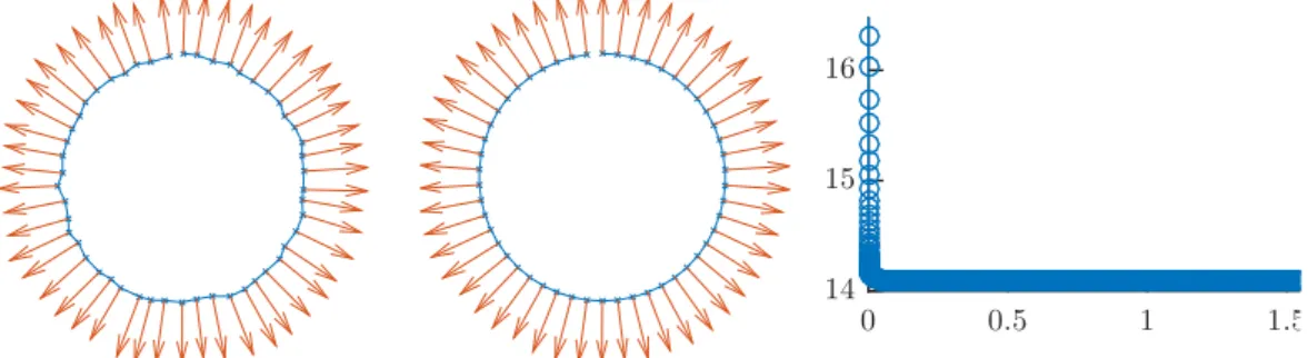
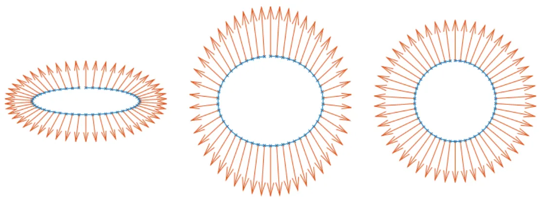
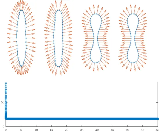
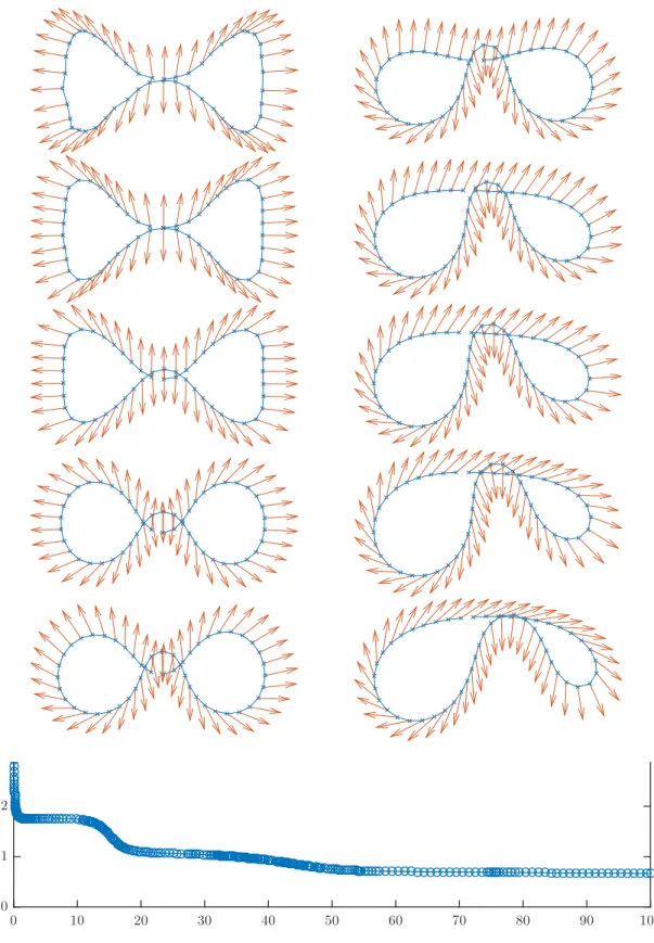
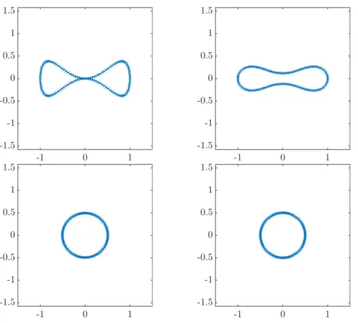
We mention this idea in particular, since it was also used in the numerical experiments presented in Appendix of this work. To get a better feeling for the behavior of different geometric flows, we used a very straight forward finite differences scheme and Matlab’s routines for ordinary differential equations to simulate the flow of curves for different evolution equations. Since mesh degeneracy becomes a problem almost immediately, we tried to account for it by the coupling to the harmonic maps heat flow.

Problems with boundary and geometric flows of networks are already present in the works of Mullins and von Neumann [71, 89] and also an import component in Euler’s [31]

study of elasticae. Strict analytical treatment of this class of problem is a main subject of a

large number of recent research projects and the analogous of long-established results for closed

manifolds are still wide open in the case of manifolds with boundaries and networks. First

analytical results were obtained by Bronsard and Reitich [13] and Mantegazza, Novaga and

Tortorelli [69].

INTRODUCTION

Organization of this Work. In the first chapter we fix some notation and introduce important mathematical concepts that appear at different points in the later chapters.

In the second chapter, we explore second-order flows that are derived from weighted surface area functionals and couple to a vector field. This will lead to a discussion of results concerning smooth anisotropic and inhomogeneous curvature flows.

In Chapter 3 we discuss important properties of the generalized Helfrich energy (3). We prove Theorem 1 and recall the gradient flow equation.

The fourth chapter is dedicated to the proof the short-time existence result as stated in Theorem 2. We start by considering the linearized equation and prove estimates for the non- linear remainder term. Together these considerations suffice to prove a first local well-posedness result. Afterwards we discuss the situation in the presence of constraints. Lastly, we employ parabolic techniques to obtain smoothness of solutions away from the initial data.

The discussion of long-time behavior of solutions in the fifth chapter is split in two parts.

For curves we prove the blow-up result as stated in Theorem 3. In the general situation of the short-time existence result, we deduce stability of local minimizers as stated in Theorem 5 by the use of the Łojasiewicz-Simon inequality.

In the Appendix, we present some numerical experiments.

Acknowledgements. During the last four years many people supported me in the process of writing this thesis.

First of all I want to thank Prof. Dr. Georg Dolzmann who primarily introduced me to the fascinating field of geometric evolution equations and who supported and encouraged me throughout my whole academic life at the University of Regensburg. I am especially grateful for many discussions that would always inspire new ideas and clarify my thoughts.

Moreover, together with the other principal investigators of the DFG-GRK 1692 “Curvature, Cycles, and Cohomology” Prof. Dr. Georg Dolzmann initiated a winterschool and a workshop on the subject of geometric evolution equations in Regensburg giving me the opportunity to make contact with the very active community of the field. Altogether I benefited heavily from my membership in the GRK enabling my to visit various inspiring conferences and invite guests to the faculty. Many ideas contributing to the progress of this work also originated from discussions at such occasions.

It was also very important to me to work in an environment where many people share my academic interests. In this context I would like to thank my colleagues, who were always on hand with help and advice and provided a very pleasant working environment. In particular, Prof. Dr. Harald Garcke and Prof. Dr. Helmut Abels were always willing to answer questions and share their experience. Besides, I would also like to thank my colleagues Fabian, Julia, Andreas, and Michael who always made time for mathematical exchange but have also been dear friends for many years.

Finally, I want to thank my parents and family for their encouragement through all the years, my wife Marina for her love, support, and understanding, and my son Antonius, who was without even knowing the greatest motivation of all while finishing this work.

9

INTRODUCTION

1

Notation and Prerequisites

In this chapter, we will introduce notation and state important definitions and theorems from geometry and analysis. Moreover, we will derive some results already tailored to the needs of later chapters, the proofs being mostly adaptions of related results from the literature.

1.1 Analysis

We adapt the usual notations of (functional) analysis. When we consider a normed space E, we denote the corresponding norm by k · k E . If E, F are Banach space, we denote the space of linear maps from E to F by L(E; F) := {A : E → F linear and continuous} with the usual operator norm, turning it into a Banach space as well. The dual space L(E, R ) is usually denoted by E ^∗ . For x ∈ E and ϕ ∈ E ^∗ we use the notations ϕ(x) and hϕ, xi E

×E to denote the application of the linear map ϕ to the element x. For an operator A ∈ L(E, F ) we denote the range and kernel of A by R(A) and ker(A), respectively. Moreover, for A ∈ L(E, F ) we introduce the adjoint operator A ^∗ ∈ L(F ^∗ , E ^∗ ) given by ϕ 7→ ϕ ◦ A.

If a map G : E → F has a Fréchet derivative it will be denoted by dG or simply G ⁰ . For d, k ∈ N and Ω ⊂ R ^d open, we denote the Jacobian of a continuously differentiable function f : Ω → R ^k by Df.

For a sequence x n in E, we denote strong and weak convergence by → and *, respectively, and if H is a Hilbert space, we denote the scalar product by h·, ·i _H .

1.2 Basic Properties of Riemannian Manifolds and Hyper- surfaces

Let M be a d-dimensional, orientable, smooth, closed manifold, that is compact without boundary.

As all manifolds in this work will be compact, we only consider connected manifolds, because

otherwise, we would do everything for all connected components separately. We denote its

tangent bundle by T M and for p ∈ M we write T p M and T _p ^∗ M for the tangent and cotangent

CHAPTER 1. NOTATION AND PREREQUISITES

space at p. For a vector bundle E over M we will denote the smooth sections of this bundle by Γ(E). For open sets V ⊂ M and U ⊂ R ^d and a chart x : V → U we denote the canonical basis vectors of T p M as ∂ x

and that of T _p ^∗ M by dx ⁱ . For k ∈ N and a smooth function f : M → R ^k , we write _∂x ^∂f

i

or shorter ∂ _i f to denote the derivatives with respect to the chart x. That is,

∂

∂x i

f (p) = ∂ i f (p) := d dt

_t=0

f (x ⁻¹ (x(p) + te i )) and we write df = f _i dx ⁱ to denote the differential of f .

If g is a Riemannian metric on M , i.e. (M, g) is a Riemannian manifold, we denote the volume element, gradient, divergence and Laplace-Beltrami operator as dµ g , ∇ g , div g , ∆ g . In particular we have for 1 ≤ p < ∞ the Banach spaces

L ^p (M ) = (

f : M → R

f measurable and kf k _L

(M) :=

Z

M

|f | ^p dµ g

^1/p

< ∞ )

. The Levi-Civita covariant derivative will be denoted by ∇ and for 1 ≤ i ≤ n we write ∇ i to mean

∇ ∂

and for k ∈ N we denote the k-th covariant derivative by ∇ ^k . The Christoffel symbols are denoted by Γ ^r _ij and they are defined by ∇ i X j = Γ i j ^r X r .

For k, r, s ∈ N and an (r, s)-tensor field T the quantity ∇ ^k T is, without further specification of vector fields with respect to which the covariant derivative is taken, an (r, s + k)-tensor. The metric induces a scalar product and norm also for tensors by

hT, Si = g ⁱ

^k

. . . g ⁱ

^k

g j

`

. . . g j

`

T _j ⁱ

_...j ^...i

S _` ^k

^...k

1

...`

and |T| = p

hT, T i for (r, s)-tensors T and S. With this we can explain the L ^p -norm also for a section X of a tensor bundle E over M by

kX k L

(M) :=

Z

M

|X| ^p dµ _g 1/p

< ∞ as well as the L ² scalar product.

For two vectors u, v ∈ R ^d+1 , we will use the notation u ⊗ v := uv ^T .

Therefore, u ⊗ v is a matrix s with entries s ij = u i v j and corresponds to the linear map R ^d+1 → R ^d+1 : x 7→ uhv, xi _R

.

We will often consider the case that M is immersed to R ^d+1 by ϕ : M → R ^d+1 . In this case the tangent space to ϕ(M ) at a point ϕ(p) ∈ R ^d+1 is given by the image of the differential T _ϕ(p) ϕ(M ) = dϕ(T _p M ) and we write

X _i := ∂ _i ϕ

for the induced basis vectors and after choosing an orientation we write ν : M → S ^d for the positively oriented unit normal to ϕ(M ). We can pull back the metric on R ^d+1 via ϕ by setting

g ij = hX i , X j i _R

.

That is, we consider the metric given by the pullback of the metric on R ^d+1 via ϕ. The pullback

is usually denoted by a ∗ symbol, hence we might write g = ϕ ^∗ h·, ·i _R

. In this case, we will

also use the notation dµ ϕ , ∇ ϕ , div ϕ , ∆ ϕ to mean the quantities related to the metric induced by

1.3. PLANE CURVES

the immersion. For immersions, we will consider the signed area functional A and the signed volume functional V at various points of this work. They are given by

A(ϕ) = Z

M

dµ _ϕ and V (ϕ) = Z

M

hϕ, ν ϕ i dµ _ϕ .

Since T ϕ(p) ϕ(M ) and T ν(p) S ^d consist of all vectors v ∈ R ^d+1 such that v ⊥ ν(p) and since T _ϕ(p) ϕ(M ) ∼ = T _p M , we can identify these spaces. The second fundamental form is the map

A : T p M × T p M → R , that is given in local coordinates by

h _ij = h ∂ ² ϕ

∂ _i ∂ _j , νi _R

= −h∂ _i ν, X _j i _R

= −g(dνX _i , X _j ).

Working with Riemannian manifolds, we will in general use the Einstein summation convention.

For example a tangential vector field v ∈ Γ(T M ) will be denoted in local coordinates as v = v ⁱ ∂ x

.Finally we introduce the mean curvature

H = g ^ij h _ij .

When M is immersed to R ^d+1 via ϕ and v : M → R ^d+1 is a smooth vector valued map, we define ∇ ϕ v and ∆ ϕ v component-wise as

∇ ϕ v =

d+1

X

α=1

e α ⊗ ∇ ϕ v ^α and ∆ ϕ v =

d+1

X

α=1

e α ⊗ ∆ ϕ v ^α . The tangential divergence is defined as usual by

div ϕ v = g ^ij h∂ i v, X j i yielding the important identity H = − div ϕ ν .

1.3 Plane Curves

Following the conventions in related literature, we will use different notation when we discuss curves. Let γ : S ¹ → R ² be a smooth map. We identify S ¹ with [0, 1] if convenient. The parameter in [0, 1] will mostly be denoted by x and we write ˙ γ(x) := _dx ^d γ(x). The length of a differentiable curve is given by L(γ) = R 1

0 | γ(x)|dx. ˙ Definition 1.1 (Regular curve)

The map γ is called a regular curve, if for all x ∈ [0, 1] we have ˙ γ(x) 6= 0.

In this case we denote the unit tangent vector by τ := _k ^γ _γk ^˙ _˙ and the unit normal by ν , where we choose the direction of ν so that (τ, ν ) has positive orientation. For plane curves, we denote the curvature by κ.

If γ is regular, it is possible to reparametrize γ by arc length. That is, there exists a strictly increasing, bijective, and smooth map α : [0, 1] → [0, L] such that k _ds ^d γ(α ⁻¹ (s))k ≡ 1. We call s the arc length parameter. For a function f : S ¹ → R smoothness means smooth in charts.

Moreover, for y ∈ S ¹ we define the arc length derivative as d

ds f _y

:= 1 k γk ˙

d dx f

_y

13

CHAPTER 1. NOTATION AND PREREQUISITES

and observe d ²

ds ² f = 1 k γ(x)k ˙

d dx

1 k γ(x)k ˙

d dx f (y)

= 1

k γ(x)k ˙ ² d ²

dx ² f − h γ, ˙ γi ¨ k γ(x)k ˙ ⁴

d

dx f. (1.1) In this notation τ = _ds ^d γ and

κ = h d

ds τ, νi = h d ² ds ² γ, νi.

The curvature κ, τ and ν are related by the Frenet equations d

ds τ = κν, d

ds ν = −κτ.

In the manifold notation from Section 1.2 we have X = d

dx γ = k γkτ, ˙ g =hX, Xi = h d

dx γ, d

dx γi = k γk ˙ ² ,

∇ _g f =g ⁻¹ d

dx f X = ( d

ds f )τ =: ∇ _s f.

If v : S ¹ → R ² is a vector field, the divergence is given by div(v) = h d

ds v, τi.

Applying this to the tangential gradient of f we find div(∇ s f ) = h d

ds d

ds f

τ

, τ i = d ² ds ² f.

1.4 Function Spaces on Manifolds

Theory of Sobolev spaces on open domains in euclidean space is explained in the books by Evans [32] or Adams [1] and the most important results carry over to the manifold setting that is e.g. treated in the Books by Aubin [5], Hebey [46] and Taylor [83–85]. For the following definitions and theorems we follow Hebey [46, Chapter 2].

Definition 1.2 (Sobolev and Hölder Spaces)

Let (M, g) be an orientable smooth closed Riemannian manifold of dimension d ∈ N . For 1 ≤ p < ∞, k ∈ N and f ∈ C ^∞ (M ) we set

kf k _W

(M ) =

k

X

j=0

k∇ ^j fk L

(M ) .

The spaces W ^k,p are defined as closures of C ^∞ (M ) with respect to these norms.

We write H ^k (M ) to denote the Hilbert spaces W ^k,2 (M ) with hf 1 , f ₂ i _H

(M) =

k

X

j=0

h∇ ^j f ₁ , ∇ ^j f ₂ i L

(M) .

Let d g : M × M → R denote the geodesic distance on (M, g). For f ∈ C ⁰ (M ), k ∈ N and α ∈ (0, 1) we set

kf k _C

(M) =

k

X

j=0

sup

p∈M

|∇ ^j f (p)| + sup

r6=s∈M

|∇ ^j f(r) − ∇ ^j f (s)|

d _g (r, s) ^α

1.5. MOVING HYPERSURFACES

and

C ^k,α (M ) =

f : M → R continuous

kf k _C

(M) < ∞

For the definition of fractional Sobolev spaces on manifolds, i.e. Besov and Bessel-potential spaces, we refer to the work of Triebel [87, 88]. In the subsequent chapters we will also use the embedding theorems of Sobolev and Morrey and the Rellich-Kondrakov theorem.

Theorem 1.3 (Theorems 2.6, 2.7, 2.8, and 2.9 from [46])

Let (M, g) be a smooth closed Riemannian manifold of dimension d ∈ N . Let k, ` ∈ N ∪ {0} with k ≥ `, 1 ≤ p, q < ∞ and α ∈ (0, 1) be fixed. If k − ^d _p ≥ ` − ^d _q , then

W ^k,p (M ) , → W <sup>`,q</sup> (M ) and if k − <sup>d</sup> <sub>p</sub> ≥ ` + α, then

W ^k,p (M ) , → C ^`,α (M ).

These embeddings are compact, if k − ^d _p > ` − <sup>d</sup> <sub>q</sub> or k − <sup>d</sup> <sub>p</sub> > ` + α, respectively.

Since we assume M to have no boundary, we state the mean value version of Poincaré’s inequality.

Theorem 1.4 (Theorem 2.10 from [46])

Let (M, g) be a smooth closed Riemannian manifold of dimension d ∈ N and fix 1 < p < ∞.

Then there is C > 0 such that for all f ∈ W ^1,p (M ) setting f ¯ := _Vol(M,g) ¹ R

fdµ g it holds that Z

M

|f − f ¯ | ^p dµ _g ^1/p

≤ C Z

M

|∇f | ^p dµ _g ^1/p

.

We will often consider immersions of smooth manifolds. For them we introduce the following notation.

Definition 1.5

Let M be a smooth, closed and orientable manifold of dimension d ∈ N , then the set of immersions is open in C ¹ (M, R ^d+1 ),we denote it by

C _imm ¹ (M, R ^d+1 ) =

ϕ ∈ C ¹ (M, R ^d+1 )

∀p ∈ M the map dϕ(p) : T p M → R ^d+1 is injective . Moreover, we have for 2 ≤ k ∈ N the Banach space

C ¹ (M, R ^d+1 ) ∩ H ^k (M, R ^d+1 )

which we equip with the usual norm k · k _C

∩H

= k · k C

+ k · k _H

. Then, the set H _imm ^k (M, R ^d+1 ) = H ^k (M, R ^d+1 ) ∩ C _imm ¹ (M, R ^d+1 ).

is open in C ¹ ∩ H ^k .

1.5 Moving Hypersurfaces

For studying the evolution of hypersurfaces, we will follow the usual approach as explained by Huisken, Polden [50, 76] or Mantegazza [68]. In the following, let M be a d-dimensional,

15

CHAPTER 1. NOTATION AND PREREQUISITES

smooth, closed, orientable manifold and ϕ : M → R ^d+1 a smooth immersion. We equip M with a Riemannian metric by pulling back the metric of R ^d+1 along ϕ as in Section 1.2. Thus, a smooth family ϕ t of immersions yields a smooth family of Riemannian manifolds (M, g t ). In the following we will discuss some formulas for the evolution of geometric quantities of (M, g _t ) as ϕ t varies in time. These formulas are well established in literature. Huisken and Polden [50]

consider the more general case where ϕ is an immersion to a higher dimensional manifold N rather than R ^d+1 , Mantegazza [68] considers essentially the situation described here and Kuwert and Schätzle [55, 56] derive their formulas in the context of immersions in euclidean space but arbitrary codimension.

Definition 1.6

Let ϕ t be a smooth family of immersions and let Ψ t := ∂ t ϕ t denote its time derivative. We can decompose Ψ t in its normal and tangential parts as

Ψ t = Ψ ^N _t ν t + Ψ ^k _t X k,t .

We say that ϕ t is a normal family of immersions if and only if the tangential part of Ψ t vanishes, i.e. for all k = 1, ..., d we have Ψ ^k _t ≡ 0.

The next lemma is a slight modification of a well known result, we follow the proof of Mantegazza [68, Proposition 1.3.4].

Lemma 1.7

For T 1 , T 2 ∈ R let (ϕ t ) _t∈[T

_,T

_] be a smooth family of immersions and let Ψ t := ∂ t ϕ t denote its time derivative. Then, for every s ∈ [T 1 , T 2 ] there exists a family F t,s : M → M of diffeomorphisms such that F _s,s = Id _M and ∂ _t (ϕ _t ◦ F _t,s ) is normal along ϕ _t (M ), that is there exists a family of functions V t,s : M → R such that ∂ t (ϕ t ◦ F t,s ) = V t,s ν t ◦ F t,s ).

Proof. We split Ψ _t in its normal and tangential part setting Ψ _t = Ψ ^N _t ν _t + Ψ ^k _t X _k,t . Hence, Ψ ^k _t X k,t is a tangential vector field along ϕ t (M ). Since ϕ t are immersions, dϕ t is invertible on its image and therefore, we can define a smooth family of vector fields on M by

Y t = −[dϕ t ] ⁻¹ Ψ ^k _t X k,t .

Since M is compact, by the theory of ordinary differential equations [59, Theorem 9.12], for every s ∈ [T 1 , T 2 ] we find a smooth family of maps F t,s : M → M satisfying

∂ t F t,s (p) = Y t (F (p)), F s,s = Id M .

By uniqueness of solutions and smooth dependence on initial data for each t ∈ [T 1 , T 2 ] the map F t,s is a smooth bijection. That it is indeed a diffeomorphism follows from the following consideration analogous to the use of the Wronski determinant in the theory of ordinary differential equations. We apply the rule for differentiation of determinants, that reads for A(t) an invertible, time dependent matrix

d

dt det(A(t)) = det(A) tr(A ⁻¹ ∂ t A(t)).

1.5. MOVING HYPERSURFACES

Thus, using F s,s = Id M and therefore det(dF s,s ) = 1 we can calculate d

dt det(dF _t,s ) = tr dF _t,s ⁻¹ d dt dF _t,s

det(dF _t,s )

= tr dF _t,s ⁻¹ d d dt F t,s

det(dF t,s )

= tr dF _t,s ⁻¹ d Y (F _t,s , t)

det(dF _t,s )

= tr dF _t,s ⁻¹ dY (F _t,s , t)dF _t,s

det(dF _t,s )

= tr dY (F t,s , t)

det(dF t,s ) and we conclude that

det(dF _t,s ) = det(Id) exp Z t

s

tr dY (F _τ,s , τ ) dτ

> 0.

Moreover, we see that

∂ t (ϕ t (F t,s )) =Ψ t (F t,s ) + dϕ t (F t,s )∂ t F t,s

=Ψ t (F t,s ) − dϕ t (F t,s )[dϕ t (F t,s )] ⁻¹ Ψ ^k _t (F t,s )X k,t (F t,s )

=Ψ ^N _t (F _t,s )ν _t (F _t,s ), that is ϕ t ◦ F t,s is normal along ϕ t (M ).

Definition 1.8

For T 1 , T 2 ∈ R and a smooth family of smooth immersions (ϕ t ) _t∈[T

_,T

_] , we call

T := [

(p,t)∈M×[T

,T

]

{p} × {ϕ t (p)} × {t}

the trajectory of ϕ _t . We say a function is a material function if its domain is M × [T ₁ , T ₂ ] and spatial if its domain is T .

Observe that with this definition the notion of a spatial function is well defined even if ϕ t is only a family of immersions rather than of embeddings.

For t ∈ R fixed, consider points x ∈ R ^d+1 and p ∈ M such that x = ϕ t (p). For a smooth function f : R ^d+1 × [T ₁ , T ₂ ] → R and a vector v ∈ R ^d+1 we denote the directional derivative by

∂ v f (x, t) := _ds ^d

_s=0 f (x+ sv, t) and the tangential gradient by ∇ g

f (x, t) := g _t ^ij (p)∂ X

f (x, t)X j,t . This yields a splitting Df (x, t) = ∇ g

f (x, t) + ∂ ν

f (x, t)ν ⊗ ν.

We have by the chain rule the identity

∂ t [f (p, ϕ t (p), t)] = ∂ t f (p, ϕ t (p), t) + ∂ ν

f (p, ϕ t (p), t)Ψ ^N _t (p) + ∇ g

f (p, ϕ t (p), t) · (Ψ ^k _t X k,t ).

For a spatial function f that is defined on the trajectory T of ϕ t it is not clear what the expression ∂ _ν

f (p, ϕ _t (p), t)Ψ ^N _t (p) should mean. To that account, a useful notion of material derivatives for quantities on trajectories is provided by Prüss and Simonett [77, §2.5.3].

Definition 1.9

Let ϕ t be a family of immersions with trajectory T and let Ψ t := ∂ t ϕ t denote its time derivative.

Let F t,s : M → M be a smooth two parameter family of diffeomorphisms of M such that F t,t = Id M and η t,s = ϕ t ◦ F t,s is normal along ϕ t (M ), whose existence is guaranteed by Lemma 1.7. For a spatial function g : T → R we call

D Dt g

_(p,ϕ(p),t)

= ∂ t (g(p, ϕ t (p), t))

17