SFB 649 Discussion Paper 2006-071
Color Harmonization in Car Manufacturing
Process
Anton Andriyashin*
Michal Benko*
Wolfgang Härdle*
Roman Timofeev*
Uwe Ziegenhagen*
* Institute for Statistics and Econometrics, School of Business and Economics, Humboldt-Universität zu Berlin, Germany
This research was supported by the Deutsche
Forschungsgemeinschaft through the SFB 649 "Economic Risk".
http://sfb649.wiwi.hu-berlin.de ISSN 1860-5664
S FB
6 4 9
E C O N O M I C
R I S K
B E R L I N
Color Harmonization in Car Manufacturing Processes ∗
A. Andriyashin, M. Benko, W. Härdle, R. Timofeev and U. Ziegenhagen October 5, 2006
One of the major cost factors in car manufacturing is the painting of body and other parts such as wing or bonnet. Surprisingly, the painting may be even more expensive than the body itself. From this point of view it is clear that car manufacturers need to observe the painting process carefully to avoid any deviations from the desired result. Especially for metallic colors where the shining is based on microscopic aluminium particles, customers tend to be very sensitive towards a difference in the light reflection of different parts of the car.
The following study, carried out in close cooperation with a partner from car industry, combines classical tests and nonparametric smoothing tech- niques to detect trends in the process of car painting. The localized versions motivated by t-test, Mann-Kendall, Cox-Stuart and a change point test are employed in this study. Suitable parameter settings and the properties of the proposed tests are studied by simulations based on resampling methods borrowed from nonparametric smoothing.
The aim of the analysis is to find a reliable technical solution which avoids any interaction from a human side.
1 Introduction
Car painting is a complex combination of different layers of base coat, color and protective finishing coat. The setup for the painting process requires the optimal adjustment of a variety of different parameters such as humidity, temperature and the consistence of the lacquer itself. Even small changes to one of these parameter may influence the adhesion of the particles and their reflection behavior.
∗This research was supported by the Deutsche Forschungsgemeinschaft through the SFB 649 ’Economic Risk’. This paper has been accepted for publication in theJournal of Applied Stochastic Models in Business and Industry
This applied paper arose from close cooperation with a partner from industry. Together we have set up a series of tests that combine approaches from local, nonparametric smoothing and classical statistical process control with the main focus to detect trends in the underlying production process. The aim is not do to detect when the process leaves a certain confidence band, the aim is to use statistical methods to detect changes before the process is going out of control.
The available dataset contains 7100 cars painted in one of 20 colors that had been col- lected during a three-week production run in August 2004 by specially trained personnel who used specialized devices that measured the color in terms ofL,a andb values.
These values describe specific colors in the so called L*a*b color space [7], standardized by theCommission Internationale de l’Eclairage in 1976. While there are different schemes for the representation of colors such as RGB, CMYK and HSB, L*a*b has the advantage to include all colors visible to the human eye, moreover RGB and CMYK color spaces are subspaces of L*a*b.
In L*a*b color space each specific color is represented by a three-dimensional vector of luminance (the gray level),aand bvalues for the red-green and blue-yellow components of the color respectively. Since each lacquer has different properties concerning the level of refraction data have been collected at five different angles for both wing and bonnet.
At the angles 15◦ and 110◦ the dataset showed huge variations. As we assume that the handling of the measuring device was difficult at these angles they have not been considered during the analysis.
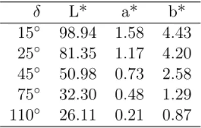
δ L* a* b*
15◦ 98.94 1.58 4.43 25◦ 81.35 1.17 4.20 45◦ 50.98 0.73 2.58 75◦ 32.30 0.48 1.29 110◦ 26.11 0.21 0.87
Table 1: L*a*b values for a ’silver’ car body measured at five different angles.
Table 1 shows an example for measurements of ’silver’ colored cars. It is worth mentioning that non-metallic colors show less differences in the values across the measurement angles.
Clearly each color needs to be analyzed separately, for simplicity we focus on a ’silver’
color in the further analysis. This laquer accounts for approximately 60% of all cars and is especially difficult to handle in the sense that even smallest differences in the refraction behavior may be detected by customers. Furthermore the analysis focuses on the L*-values, since this component plays the dominant role in gray and silver laquers.
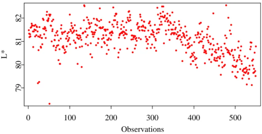
Figure 1 depicts the L*-values for a sequence of 550 silver colored cars, measured at a unique point on the bodies. Visually one might consider observation number 350 as the starting point for a trend. The x-axis shows the index of the observation. According to our partners there are no interdependencies between the lacquers in the production process.
0 100 200 300 400 500 Observations
79808182
L*
Figure 1: Data sequence of 550 L* observations, angle 25◦
The paper has the following structure. Section 2 gives an overview of proposed tests, introduces a localization framework and comments on the evaluation of test results. In section 3 the behavior of proposed tests is analyzed using simulation study. Concluding remarks are given in section 4.
2 Tests
The first test considered here is motivated by standard slope coefficient test (t-test) in the linear regression model. Clearly linearity cannot be assumed globally for the whole dataset, see figure 1). Therefore a local version of this test, an approach borrowed from smoothing methods in nonparametric regression is proposed, for details see [2]. As it will be seen in the following text, the localization of this test depends on the window size (also called bandwidth or smoothing parameter). In order to relax this dependence, a modification (called ’slope’-test) is proposed, where for each point the significance of the local slope (first derivative of the mean function) is tested using three different window sizes.
Both of these tests focus on the significance of the slope. Focusing directly on the detection of jumps (discontinuity point), local versions of Cox-Stuart, change point and Mann-Kendall test were used in addition.
The following model is assumed:
yi =m(xi) +εi E(εi) = 0,var(εi)<∞ (1) with the conditional mean functionE(yi|xi) =m(xi) and the error term εi. yi denotes the dependent variable measured at the pointxi.
Strictly speaking, in the car painting application the data were measured and collected car-by-car without considering the exact time point of measurement.
Hence the following notation would be sufficient:
yi =mi+εi E(εi) = 0,var(εi)<∞ (2) with the mean functionE(yi) =miand the error termεi. yidenotes the observed variable (L* value). However notation in the form of (1) is more convenient for introducing the localization framework. Note that the equation (2) can be represented in the form of (1) simply by settingxi =i.
2.1 t-test
The basic idea behind the t-test is to test whether the slopeβ1 of the linear model:
m(x) =β0+β1x is significantly different from zero.
Estimators of the linear regression line are obtained by minimizing the sum of squares:
(βc0,cβ1) = arg min
β0,β1
n
X
i=1
(yi−β0−β1xi)2. (3) Under the null hypothesisβ1 = 0 the test statistics follows the t-distribution withn−2 degrees of freedom.
Strictly speaking thet-distribution of the test statistics relies on normality assumption of the dependent variables yi, however it is known that the t-test is relatively robust towards slight violation of this assumption.
Local t-test While formula (3) shows the global setup for t-test, local versions allowing to relax the assumptions on the conditional mean functionm in (2) are employed for all tests in this study.
Referring to [1] for technical details, one can motivate the localized setup as follows. In- stead of assuming the linearity ofmglobally, i.e. assumingm(x) =β0+β1x, x∈[x0, xn], one pointx is fixed and one essentially assumes thatmcan be approximated sufficiently well in the small neighborhood (window) aroundx. Alternatively this approach can be motivated by allowing the coefficients β0, β1 to change, depending on the point x, i.e.
β0,x, β1,x.
In the car painting application the localization is performed on the set of (design) pointsxl=x0+l∆,l= 1, . . . , n/L. For each pointxltheβ0,xl, β1,xl are calculated using observations from window ofL cases only. More formally, (3) is modified to:
βd0,xl,βd1,xl
= arg min
β0,β1
n
X
i=1
(yi−β0−β1xi)2I(xi∈Ll) (4) where I denotes the indicator function andLl = [x0+ (l−1)·∆, x0+ (l−1)·∆ +L], l= 1. . .n/L. Please note that the car painting application is a quality control problem, therefore only the left neighborhood (history w.r.t. point xl) can be used to signal a
significant trend, see construction of the intervalLlabove. In the classical local smoothing the localization window is typically centered around the point xl.
The approach can be generalized by additional weighting of the points in the localiza- tion window, e.g. the weights can be set smaller for observations that are far away from pointxland consequently higher for points close toxl. This can be done by introduction of the kernel functionK(·), see [2] for details. The estimation procedure can be rewritten as:
βd0,xl,βd1,xl
= arg min
β0,β1
n
X
i=1
(yi−β0−β1xi)2K
xi−xl
h 1
h. (5)
Typically the kernel function is a symmetric (in classical regression problems) density function with compact support, Gaussian probability density function is also a popular choice. The parameterh is a so called bandwidth and can be regarded as the half of the localization window.
It is a well known fact that the bandwidth h has a crucial influence on the result.
Large values ofh yield a smooth but possibly highly biased estimator while small values of h lead to less biased but also less smooth results. For broader discussion of the local polynomial smoothing properties and optimal bandwidth choice refer to [1].
Note that t-test relies on the assumption that the errors (εi) are not correlated. To verify this condition Durbin-Watson test for three different windows with different localization windows was conducted. At the 95% confidence level the hypothesis of autocorrelation of the errors was rejected.
2.2 Slope Test
In order to reduce the influence of the bandwidth selection problem, a modification of t- test where the slope is tested at each pointxl using three different bandwidths (widths of the localization window) simultaneously is proposed. The idea of using different smooth- ing parameters in the testing problems, to authors best knowledge was first proposed by [6] and referred to as ’significant trace’.
For simplicity reasons this procedure is presented using the first setup of the test from equation (4), i.e. uniform kernel function (identity function). The generalization to an arbitrary kernel function is straightforward.
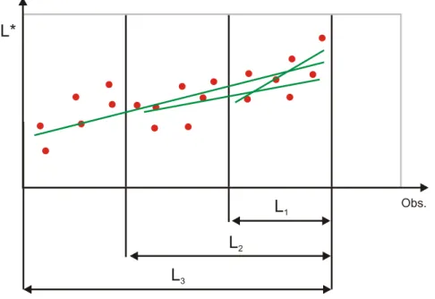
The slope test refines the idea of t-test by using 3 different window sizes for each pointxl with lengths1/3·L,2/3·L and L, see figure 2. For each of these three intervals denoted by L1, L2 and L3 the t-statistics is computed, and a significant trend for the window L is imputed if all the three test procedures show a significant deviation from zero simultaneously. Due to the simultaneousness of three procedures an adjustment of the significance levelα in the form of Bonferroni correction is required: αi =α/3where α is the (overall) desired confidence level for a test (e.g. 5%) and αi is the confidence level of each of three t-subtests.
Figure 2: Basic idea of slope test
2.3 Change Point Test
The following three tests (change point, Mann-Kendall and Cox-Stuart) will be intro- duced only in the global setup, however all of them are localized in the same way as the t-test described above.
While t-test and slope test detect trends focusing on the slope of the underlying process, these tests may be inappropriate in situations where the change in the production process is not reflected by a change of the slope but instead by a sudden jump (discontinuity point). Therefore a test that examines the means of subgroups inside the dataset is added to the portfolio of tests.
The change point test processes the data in the following way: The observations are divided into two intervalsL1 andL2. The number of observation in L1 is denoted byn1, the number of observations in L2 by n2.
For each of the two intervals the sample mean is calculated:
µcj =n−1j
nj
X
i=1
yi for yi ∈Lj, j ∈ {1,2}.
The null hypothesis of equality of the true meansµ1=µ2 versus the alternative hypoth- esisµ1 6=µ2 in the intervals is tested. The resulting test statisticsV has an asymptotic χ2 distribution with one degree of freedom.
V= n1·n2
n1+n2
(µc1−µc2)2
˜ σ2
−→L χ2(1)
The unknown standard error of the residualsσ˜ is estimated by the sample variance of the residuals from nonparametric regression (see [4]). The residualri,h equals the difference of the observed value yi and the estimated value dmh(xi).
ri,h=yi−dmh(xi) (6)
withdmh(xi) denoting the Nadaraya-Watson estimator:
dmh(xi) = P
jKxj−xh iyj
P
jKxj−xh i
with kernel functionK. The bandwidthhis computed using cross-validation, for details refer to [4].
2.4 Mann-Kendall Test
This classical approach for trend detection compares the differences of subsequent obser- vation and makes a statement on the trend using the proportion of positive differences among all computed differences. The test statistics is given by:
S =
n
X
i=2 i−1
X
j=1
sign(yi−yj) (7)
Tabulated critical values are given in [5], forn→ ∞the distribution of the test statistics converges to the standard normal distribution.
S∗ = S
qn(n−1)(2n+5) 18
−→L N(0,1) (8)
2.5 Cox-Stuart Test
While the Mann-Kendall test analyzes the differences of subsequent observations, the Cox-Stuart test uses two partitions of the underlying sample to detect trends. From the sequence of observationsy1, . . . , ynthe dividing observationmis calculated as following:
m= ( n
2 if nis even
n+1
2 if nis odd (9)
Usingmone can set up the two groups and calculate the differencesdiof the observations from the two partitions.
di= (yi+m−ym) for
( 1, . . . , m if nis even
1, . . . , m−1 if nis odd (10) The test statisticsT is then obtained as the number of all positivedi, the null hypothesis H0 of ’no trend’ is rejected if:
T <1/2
l−z1−α/2
√
l or T > l−1/2
l−z1−α/2
√
l (11)
with l being the number of non-zero di and z1−α/2 as the 1−α/2 quantile of standard normal distribution.
2.6 Evaluation of Test Results
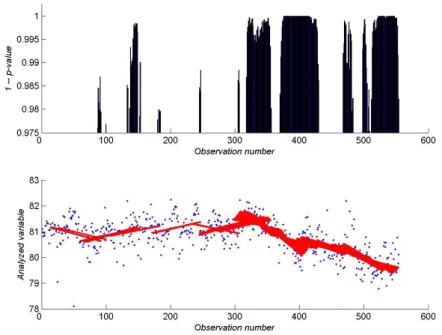
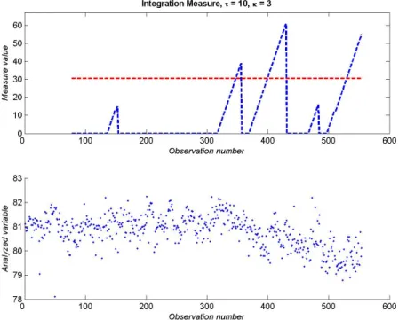
For the evaluation of the test results the following heuristics is proposed – a persistent trend should cause not just a single signal but a series of subsequent signals. To formalize this idea a summation measure is proposed. While a test generates a signal with a respective inverse p-value (i.e. 1−p where p is the p-value), the summation measure sums up significant (inverse) p-values sequentially. Significant means that1−p≥1−α or equivalentlyp≤α whereα is the confidence level.
As an example of such setup consider an example for t-test on figure 3 where a sequence of 550 observations is used. The window sizeLis 75 observations, the stepsize ∆of this window is set to 1, the significance level is 5%.
The lower part of figure 3 contains the observations and a slope line for each significant test, these lines are colored with red.
Figure 3: t-test results of the dataset
At this point one has to think carefully about the treatment of blanks (non-significant p-values) in sequences of p-values. What if there is a cluster of 10 significant p-values with a single insignificant oneinside– should then the summation measure stop at every first
absence of signal or be more flexible allowing some noise inside? If so, to what extent?
The other question is what the minimum number of consequent significant p-values is to form a trend message, because one or two indications may be false alarms?
Therefore two additional parameters are introduced to address this issue. Let τ denote the minimum number of subsequent signals (significant p-values) that is eligible for cre- ation of non-zero summation measure andκbe the maximum number of tolerated blanks (insignificant p-values).
Although the general idea of aggregation of the information from the individual test is now available, a critical value to indicate a persistent trend is clearly needed. It is worth pointing out that this value is certainly dependent on bothτ and κ.
Let us refer to an example of on figure 4 where summation measure is computed with κ= 3 andτ = 10.
Figure 4: Summation measure for the t-test results from figure 3
Looking at the summed inverse p-values depicted in figure 4 (the dashed line at the upper part), one can assume the existence of a persistent trend if the height of the sum breaks a certain limit, a threshold value η. Clearly the heuristical approach of the summation method makes it difficult to determine the critical value. After discussion with industry the following rule of thumb was used for the threshold value – 50% of the maximum value of the summation measure. In practice this value is surely inappropriate since the maximum value of the sum is not known in advance, whereas it serves quite well for the estimation of internal test localizing parameters (see below).
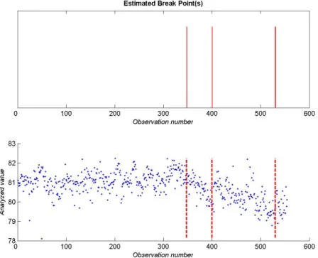
Figure 4 shows an example of the threshold value. Summed values that exceed 50%
threshold are marked using vertical red bars on figure 5.
Figure 5: Generated signals for the t-test results from figure 3 using the summation measure.
3 Simulation
The main goal of this section is to perform simulations, essentially to study the detection power of the available tests. Our analysis is based on pseudo-residual resampling. In addition the simulations have also been used to determine the internal test parameters.
For the comparison of the different tests simulated datasets are used. The basic struc- ture of each dataset consists of 550 observations, the first 300 observations have no trend (slope = 0), beginning from observation number 301 an artificial trend with slope of angle γ is added. The quality of performed test is measured by the delay - the number of observations after observation 300 until the trend has been detected.
One can argue that the residualsεi, see (2), can be modeled as normally i.i.d. However, it will be shown in the following paragraph that this does not coincide with the data set observed in the car painting application.
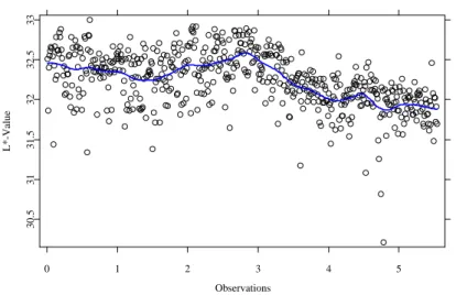
The residuals εi are estimated byri,h, see (6), i.e. as the differences between original and smoothed data, see figure 6.
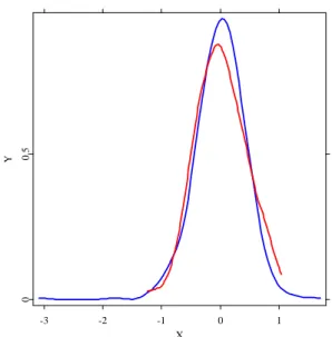
Figure 7 shows the nonparametric estimate of the density estimated from ri,h, i = 1, . . . , N and the normal density estimated from the same sample. The nonparametric estimate is obtained by the kernel density estimator, see [2]. To be able to compare these parametric and nonparametric estimates the same level of bias needs to be achieved.
Hence the normal density is additionally smoothed with the same settings for kernel and bandwidth as in the nonparametric estimate (for further discussion see [3]). Figure 7 shows the clear difference between these two densities.
Using the Jarque-Bera and Kolmogorov-Smirnov tests, the residuals were examined for normality. Since both tests rejected the normality hypothesis at the 95% confidence level, it is inappropriate to generate simulated data using normally distributed residuals.
Although one could use a broader class of parametric density functions to fit the residuals, it was decided to employ a resampling method to obtain datasets with the same random residual structure as the original data.
Simulated data noise was constructed by sampling with replacement from the estimated residualsri,h. The drawn residual was returned back to the pool so that there is a positive probability of choosing the same residual more than one time.
0 1 2 3 4 5
Observations
30.53131.53232.533
L*-Value
Figure 6: Original data (black points) and smoothed curve (blue solid curve).
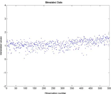
During the simulations three angles were employed to create artificial datasets: tanγ = 0.002(0.1145◦, see figure 8), tanγ = 0.005(0.2864◦) andtanγ = 0.05(2.8624◦).
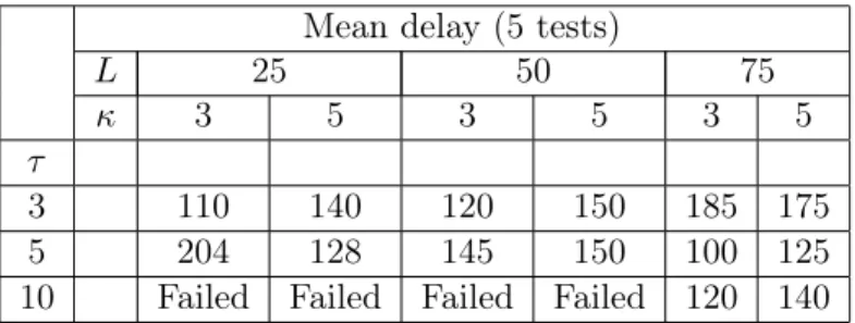
Table 2 summarizes the simulation results for internal test parameter estimation. For each set of parameters 50 simulations were performed. Let mean delay be defined as an average delay for 5 performed tests: t-test, slope test, change point test, Mann-Kendall test and Cox-Stuart test. For tanγ = 0.05 (Tables 4) the parameters L and κ had no significant influence on the mean delay, bigger values for τ gave smaller average delays.
For the two small angles tanγ = 0.002 and tanγ = 0.005 (Tables 2 and 3) some of the tests gave inconsistent results, that can be traced back to the dependance of the threshold valueη from κand ∆.
-3 -2 -1 0 1 X
00.5
Y
Figure 7: Kernel density estimation for the original dataset Mean delay (5 tests)
L 25 50 75
κ 3 5 3 5 3 5
τ
3 110 140 120 150 185 175
5 204 128 145 150 100 125
10 Failed Failed Failed Failed 120 140 Table 2: Test efficiency for simulated data with tanγ = 0.002
Since for each test a big number of simulations was conducted, aggregated results of test efficiency are provided in Figure 9. Each boxplot was built independently for each test over all performed simulations across different parameter valuesγ, L, κ, τ.
Apart from mean delay evidence, it is of great interest to investigate the behaviour of proposed tests in respect to false alarms. As before 50 simulations for each of five tests were conducted, where the average false alarm statistics for a given set of parameters was calculated.
Recall that in our simulations first 300 observations contain no trend while the last 250 observations constitute a trend with a given slope γ. Any signal before the observation number 300 generated by a procedure is acknowledged as a false alarm. Note, however, that there is no further need to compute this statistics for differrent slope angles since by definition false alarms can only occur before the beginning of the trend. In the table below, an averaged number of false alarms is provided, where averaging was performed over the number of simulations and the number of tests.
Figure 8: Simulated data with angletanγ = 0.002 Mean delay (5 tests)
L 25 50 75
κ 3 5 3 5 3 5
τ
3 130 170 150 120 215 225
5 160 125 100 115 145 145
10 Failed Failed 130 120 90 95
Table 3: Test efficiency for simulated data with tanγ = 0.005
Mean number of false alarms
L 25 50 75
κ 3 5 3 5 3 5
τ
1 2.3 1.9 2.1 1.7 1.1 0.5
2 1.2 0.6 1.0 0.4 0.3 0
3 0 0 0 0 0 0
5 0 0 0 0 0 0
10 0 0 0 0 0 0
Table 5: False alarm statistics for simulated data
Mean delay (5 tests)
L 25 50 75
κ 3 5 3 5 3 5
τ
3 110 140 120 150 185 175
5 204 128 145 150 100 125
10 Failed Failed Failed Failed 120 140 Table 4: Test efficiency for simulated data with tanγ = 0.05
Figure 9: Boxplots for test delays of five performed tests
The main conclusion one can draw from this table is that proper adjusted integration measure parameters (τ andκ) can effectively avoid false alarms. In case whenτ = 1the integration measure is in fact no longer employed. Enough big τ and κ make it possible to eliminate single false signals and therefore the proposed procedures work effectively in this regard.
4 Conclusions
The best performance has been shown by t-test, change-point test and slope test, there- fore we recommended the simultaneous use of these three tests to our partner. The detection power of Mann-Kendall and Cox-Stuart test was below the power of the first three tests so this pair was not recommended for usage in a given situation.
The t-test showed good results in most of the simulation runs, also it is fast to compute.
For outliers and small window sizes L it proved to be inefficient, because it is based on the linear regression model.
The change point tests showed the best results on average. The drawback of this test is that it is slow and difficult in computation, sinceσbhas to be computed from the data and it tends to generate single false signals, therefore the test parameters need to be adjusted carefully. But due to the employment of summation measure, single false signals are not transformed into false alarms. Therefore the majority of false alarms could be avoided.
All tests showed a dependence on the setup for L,κ and τ, values for L= 75,κ = 5 and τ = 3 showed good results.
Further research has to provide suitable ranges for the threshold value, the used 50%
of the maximum summation measure value was only employed as initial proposal.
References
[1] Fan J, and Gijbels I Local Polynomial Modelling and its Applications Chapman &
Hall, 1996
[2] Härdle WApplied Nonparametric Regression Cambridge University Press, 1990 [3] Härdle W, Mammen ETesting parametric versus nonparametric regression Annals
of Statistics 21: 1926-1947 (1993)
[4] Härdle W, Müller M, Werwatz A Nonparametric and Semiparametric Models Springer, 2004
[5] Hollander M, Wolfe DNonparametric Statistical Methods Wiley, 1973
[6] King E, Hart J, Wehrly TTesting the equality of two regression curves using linear smoother Statist. Probab. Lett. 12 239-247 (1991)
[7] McLaren K The development of the CIE 1976 (L*a*b*) uniform color space and color-difference formula Journal of the Society of Dyers and Colorists 92, 338-341 (1976)
SFB 649 Discussion Paper Series 2006
For a complete list of Discussion Papers published by the SFB 649, please visit http://sfb649.wiwi.hu-berlin.de.
001 "Calibration Risk for Exotic Options" by Kai Detlefsen and Wolfgang K.
Härdle, January 2006.
002 "Calibration Design of Implied Volatility Surfaces" by Kai Detlefsen and Wolfgang K. Härdle, January 2006.
003 "On the Appropriateness of Inappropriate VaR Models" by Wolfgang Härdle, Zdeněk Hlávka and Gerhard Stahl, January 2006.
004 "Regional Labor Markets, Network Externalities and Migration: The Case of German Reunification" by Harald Uhlig, January/February 2006.
005 "British Interest Rate Convergence between the US and Europe: A Recursive Cointegration Analysis" by Enzo Weber, January 2006.
006 "A Combined Approach for Segment-Specific Analysis of Market Basket Data" by Yasemin Boztuğ and Thomas Reutterer, January 2006.
007 "Robust utility maximization in a stochastic factor model" by Daniel Hernández–Hernández and Alexander Schied, January 2006.
008 "Economic Growth of Agglomerations and Geographic Concentration of Industries - Evidence for Germany" by Kurt Geppert, Martin Gornig and Axel Werwatz, January 2006.
009 "Institutions, Bargaining Power and Labor Shares" by Benjamin Bental and Dominique Demougin, January 2006.
010 "Common Functional Principal Components" by Michal Benko, Wolfgang Härdle and Alois Kneip, Jauary 2006.
011 "VAR Modeling for Dynamic Semiparametric Factors of Volatility Strings"
by Ralf Brüggemann, Wolfgang Härdle, Julius Mungo and Carsten Trenkler, February 2006.
012 "Bootstrapping Systems Cointegration Tests with a Prior Adjustment for Deterministic Terms" by Carsten Trenkler, February 2006.
013 "Penalties and Optimality in Financial Contracts: Taking Stock" by Michel A. Robe, Eva-Maria Steiger and Pierre-Armand Michel, February 2006.
014 "Core Labour Standards and FDI: Friends or Foes? The Case of Child Labour" by Sebastian Braun, February 2006.
015 "Graphical Data Representation in Bankruptcy Analysis" by Wolfgang Härdle, Rouslan Moro and Dorothea Schäfer, February 2006.
016 "Fiscal Policy Effects in the European Union" by Andreas Thams, February 2006.
017 "Estimation with the Nested Logit Model: Specifications and Software Particularities" by Nadja Silberhorn, Yasemin Boztuğ and Lutz Hildebrandt, March 2006.
018 "The Bologna Process: How student mobility affects multi-cultural skills and educational quality" by Lydia Mechtenberg and Roland Strausz, March 2006.
019 "Cheap Talk in the Classroom" by Lydia Mechtenberg, March 2006.
020 "Time Dependent Relative Risk Aversion" by Enzo Giacomini, Michael Handel and Wolfgang Härdle, March 2006.
021 "Finite Sample Properties of Impulse Response Intervals in SVECMs with Long-Run Identifying Restrictions" by Ralf Brüggemann, March 2006.
022 "Barrier Option Hedging under Constraints: A Viscosity Approach" by Imen Bentahar and Bruno Bouchard, March 2006.
SFB 649, Spandauer Straße 1, D-10178 Berlin http://sfb649.wiwi.hu-berlin.de
023 "How Far Are We From The Slippery Slope? The Laffer Curve Revisited"
by Mathias Trabandt and Harald Uhlig, April 2006.
024 "e-Learning Statistics – A Selective Review" by Wolfgang Härdle, Sigbert Klinke and Uwe Ziegenhagen, April 2006.
025 "Macroeconomic Regime Switches and Speculative Attacks" by Bartosz Maćkowiak, April 2006.
026 "External Shocks, U.S. Monetary Policy and Macroeconomic Fluctuations in Emerging Markets" by Bartosz Maćkowiak, April 2006.
027 "Institutional Competition, Political Process and Holdup" by Bruno Deffains and Dominique Demougin, April 2006.
028 "Technological Choice under Organizational Diseconomies of Scale" by Dominique Demougin and Anja Schöttner, April 2006.
029 "Tail Conditional Expectation for vector-valued Risks" by Imen Bentahar, April 2006.
030 "Approximate Solutions to Dynamic Models – Linear Methods" by Harald Uhlig, April 2006.
031 "Exploratory Graphics of a Financial Dataset" by Antony Unwin, Martin Theus and Wolfgang Härdle, April 2006.
032 "When did the 2001 recession really start?" by Jörg Polzehl, Vladimir Spokoiny and Cătălin Stărică, April 2006.
033 "Varying coefficient GARCH versus local constant volatility modeling.
Comparison of the predictive power" by Jörg Polzehl and Vladimir Spokoiny, April 2006.
034 "Spectral calibration of exponential Lévy Models [1]" by Denis Belomestny and Markus Reiß, April 2006.
035 "Spectral calibration of exponential Lévy Models [2]" by Denis Belomestny and Markus Reiß, April 2006.
036 "Spatial aggregation of local likelihood estimates with applications to classification" by Denis Belomestny and Vladimir Spokoiny, April 2006.
037 "A jump-diffusion Libor model and its robust calibration" by Denis Belomestny and John Schoenmakers, April 2006.
038 "Adaptive Simulation Algorithms for Pricing American and Bermudan Options by Local Analysis of Financial Market" by Denis Belomestny and Grigori N. Milstein, April 2006.
039 "Macroeconomic Integration in Asia Pacific: Common Stochastic Trends and Business Cycle Coherence" by Enzo Weber, May 2006.
040 "In Search of Non-Gaussian Components of a High-Dimensional Distribution" by Gilles Blanchard, Motoaki Kawanabe, Masashi Sugiyama, Vladimir Spokoiny and Klaus-Robert Müller, May 2006.
041 "Forward and reverse representations for Markov chains" by Grigori N.
Milstein, John G. M. Schoenmakers and Vladimir Spokoiny, May 2006.
042 "Discussion of 'The Source of Historical Economic Fluctuations: An Analysis using Long-Run Restrictions' by Neville Francis and Valerie A.
Ramey" by Harald Uhlig, May 2006.
043 "An Iteration Procedure for Solving Integral Equations Related to Optimal Stopping Problems" by Denis Belomestny and Pavel V. Gapeev, May 2006.
044 "East Germany’s Wage Gap: A non-parametric decomposition based on establishment characteristics" by Bernd Görzig, Martin Gornig and Axel Werwatz, May 2006.
045 "Firm Specific Wage Spread in Germany - Decomposition of regional differences in inter firm wage dispersion" by Bernd Görzig, Martin Gornig and Axel Werwatz, May 2006.
SFB 649, Spandauer Straße 1, D-10178 Berlin http://sfb649.wiwi.hu-berlin.de
046 "Produktdiversifizierung: Haben die ostdeutschen Unternehmen den Anschluss an den Westen geschafft? – Eine vergleichende Analyse mit Mikrodaten der amtlichen Statistik" by Bernd Görzig, Martin Gornig and Axel Werwatz, May 2006.
047 "The Division of Ownership in New Ventures" by Dominique Demougin and Oliver Fabel, June 2006.
048 "The Anglo-German Industrial Productivity Paradox, 1895-1938: A Restatement and a Possible Resolution" by Albrecht Ritschl, May 2006.
049 "The Influence of Information Costs on the Integration of Financial Markets: Northern Europe, 1350-1560" by Oliver Volckart, May 2006.
050 "Robust Econometrics" by Pavel Čížek and Wolfgang Härdle, June 2006.
051 "Regression methods in pricing American and Bermudan options using consumption processes" by Denis Belomestny, Grigori N. Milstein and Vladimir Spokoiny, July 2006.
052 "Forecasting the Term Structure of Variance Swaps" by Kai Detlefsen and Wolfgang Härdle, July 2006.
053 "Governance: Who Controls Matters" by Bruno Deffains and Dominique Demougin, July 2006.
054 "On the Coexistence of Banks and Markets" by Hans Gersbach and Harald Uhlig, August 2006.
055 "Reassessing Intergenerational Mobility in Germany and the United States: The Impact of Differences in Lifecycle Earnings Patterns" by Thorsten Vogel, September 2006.
056 "The Euro and the Transatlantic Capital Market Leadership: A Recursive Cointegration Analysis" by Enzo Weber, September 2006.
057 "Discounted Optimal Stopping for Maxima in Diffusion Models with Finite Horizon" by Pavel V. Gapeev, September 2006.
058 "Perpetual Barrier Options in Jump-Diffusion Models" by Pavel V.
Gapeev, September 2006.
059 "Discounted Optimal Stopping for Maxima of some Jump-Diffusion Processes" by Pavel V. Gapeev, September 2006.
060 "On Maximal Inequalities for some Jump Processes" by Pavel V. Gapeev,
September 2006.
061 "A Control Approach to Robust Utility Maximization with Logarithmic Utility and Time-Consistent Penalties" by Daniel Hernández–Hernández and Alexander Schied, September 2006.
062 "On the Difficulty to Design Arabic E-learning System in Statistics" by Taleb Ahmad, Wolfgang Härdle and Julius Mungo, September 2006.
063 "Robust Optimization of Consumption with Random Endowment" by Wiebke Wittmüß, September 2006.
064 "Common and Uncommon Sources of Growth in Asia Pacific" by Enzo Weber, September 2006.
065 "Forecasting Euro-Area Variables with German Pre-EMU Data" by Ralf Brüggemann, Helmut Lütkepohl and Massimiliano Marcellino, September 2006.
066 "Pension Systems and the Allocation of Macroeconomic Risk" by Lans Bovenberg and Harald Uhlig, September 2006.
067 "Testing for the Cointegrating Rank of a VAR Process with Level Shift and Trend Break" by Carsten Trenkler, Pentti Saikkonen and Helmut Lütkepohl, September 2006.
068 "Integral Options in Models with Jumps" by Pavel V. Gapeev, September 2006.
069 "Constrained General Regression in Pseudo-Sobolev Spaces with Application to Option Pricing" by Zdeněk Hlávka and Michal Pešta, September 2006.
SFB 649, Spandauer Straße 1, D-10178 Berlin http://sfb649.wiwi.hu-berlin.de
070 "The Welfare Enhancing Effects of a Selfish Government in the Presence of Uninsurable, Idiosyncratic Risk" by R. Anton Braun and Harald Uhlig,
September 2006.
071 "Color Harmonization in Car Manufacturing Process" by Anton Andriyashin, Michal Benko, Wolfgang Härdle, Roman Timofeev and Uwe Ziegenhagen, October 2006.
SFB 649, Spandauer Straße 1, D-10178 Berlin http://sfb649.wiwi.hu-berlin.de