Zooplankton Gut Passage Mobilizes Lithogenic Iron for Ocean Productivity

(1)

Report

Zooplankton Gut Passage Mobilizes Lithogenic Iron for Ocean Productivity

Highlights

d Iron content in krill muscle rises with the amount of ingested lithogenic particles

d Krill feces have5-fold higher proportions of labile iron than intact diatoms

d Lithogenic iron mobilized by krill can enter the dissolved pool via multiple pathways

d The prevailing foodweb structure plays an important role in ocean iron fertilization

Authors

Katrin Schmidt, Christian Schlosser, Angus Atkinson, Sophie Fielding, Hugh J. Venables, Claire M. Waluda, Eric P. Achterberg

Correspondence

katsch@sahfos.ac.uk (K.S.), aat@pml.ac.uk (A.A.)

In Brief

Lack of iron limits primary production in the ocean. Terrestrial-derived lithogenic particles can be iron-rich, but low solubility makes it unavailable. Schmidt et al. show that zooplankton ingests these particles and acidic digestion mobilizes the attached iron. This is a significant pathway of new iron supply and can boost ocean productivity.

Schmidt et al., 2016, Current Biology26, 2667–2673 October 10, 2016ª2016 Elsevier Ltd.

http://dx.doi.org/10.1016/j.cub.2016.07.058

(2)

Current Biology

Report

Zooplankton Gut Passage Mobilizes Lithogenic Iron for Ocean Productivity

Katrin Schmidt,^1,2,6,*Christian Schlosser,^3,4Angus Atkinson,^1,5,*Sophie Fielding,¹Hugh J. Venables,¹Claire M. Waluda,¹ and Eric P. Achterberg^3,4

1British Antarctic Survey, Madingley Road, High Cross, Cambridge CB3 0ET, UK

2Sir Alister Hardy Foundation for Ocean Science, The Laboratory, Citadel Hill, Plymouth PL1 2PB, UK

3Ocean and Earth Sciences, National Oceanography Centre Southampton, University of Southampton, Southampton SO14 3ZH, UK

4GEOMAR Helmholtz Centre for Ocean Research Kiel, Wischhofstr.1-3, 24148 Kiel, Germany

5Plymouth Marine Laboratory, Prospect Place, The Hoe, Plymouth PL1 3DH, UK

6Lead Contact

*Correspondence:katsch@sahfos.ac.uk(K.S.),aat@pml.ac.uk(A.A.) http://dx.doi.org/10.1016/j.cub.2016.07.058

SUMMARY

Iron is an essential nutrient for phytoplankton, but low concentrations limit primary production and associated atmospheric carbon drawdown in large parts of the world’s oceans [1, 2]. Lithogenic particles deriving from aeolian dust deposition, glacial runoff, or river discharges can form an important source if the attached iron becomes dissolved and therefore bioavailable [3–5]. Acidic digestion by zooplankton is a potential mechanism for iron mobilization [6], but evidence is lacking. Here we show that Antarctic krill sampled near glacial outlets at the island of South Georgia (Southern Ocean) ingest large amounts of lithogenic particles and contain 3-fold higher iron concentrations in their muscle than specimens from offshore, which confirms mineral dissolution in their guts. About 90% of the lithogenic and biogenic iron ingested by krill is passed into their fecal pellets, which contain 5-fold higher proportions of labile (reactive) iron than intact diatoms. The mobilized iron can be released in dissolved form directly from krill or via multiple pathways involving microbes, other zooplankton, and krill predators. This can deliver substantial amounts of bioavailable iron and contribute to the fertilization of coastal waters and the ocean beyond. In line with our findings, phytoplankton blooms downstream of South Georgia are more intensive and longer lasting during years with high krill abundance on-shelf. Thus, krill crop phytoplankton but boost new production via their nutrient supply.

Understanding and quantifying iron mobilization by zooplankton is essential to predict ocean productivity in a warming climate where lithogenic iron inputs from deserts, glaciers, and rivers are increasing [7–10].

RESULTS AND DISCUSSION

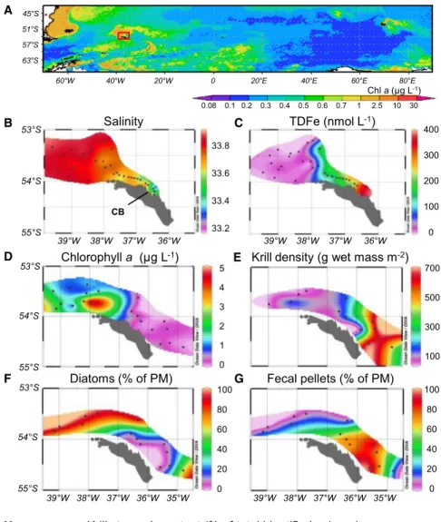
While most of the remote Southern Ocean is a high-nitrate low- chlorophyll (HNLC) area, primary productivity can be elevated

for hundreds of kilometers downstream of islands, including South Georgia (Figure 1A). This is considered a consequence of iron supply from the island shelves and its subsequent transport and recycling within the current flow [11–15]. Our in situ measurements of dissolved iron (DFe; <0.2mm), total dissolvable iron (TDFe; unfiltered), and surface water salinity suggest that high iron concentrations over the northern shelf of South Georgia are also associated with a freshwater source: melting glaciers (Figures 1B and 1C;Figure S1). Glacial runoff has been found to be an important iron source in other polar regions [4, 16, 17]

due to its high sediment load and the attached aggregations of iron oxyhydroxide nanoparticles [4, 18]. However, most of the iron associated with glacial runoff is removed from surface waters during transition from low to high salinity [19], and the fate and chemical processing of iron during transport from glaciers to the adjacent ocean is not well understood [20].

Antarctic krill (Euphausia superba) are central within the South Georgia foodweb because they transfer primary production to higher trophic levels, including fish, seals, penguins, albatrosses, and whales [21]. Highest krill abundances on the eastern side of the island coincide with low chlorophylla(chla) concentrations and the dominance of fecal pellets in the suspended matter of surface waters, which indicates intensive grazing by krill (Figures 1D–1G). However, stomach content analysis reveals that krill do not only feed on phytoplankton but also ingest lithogenic particles and copepods when those are abundant (Figure 1H).

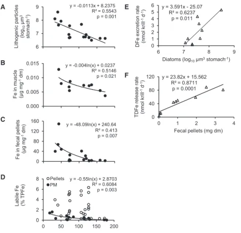
Consequently, the amount of lithogenic particles in krill stomachs increased exponentially toward the main glacial outlets at Cumberland Bay, reaching >100-fold higher values than at a reference station 170 km away (Figure 2A). In concert with the increased ingestion of lithogenic particles, krill had up to 3-fold higher iron concentrations in their muscle tissue and 1–2 orders of magnitude higher iron concentrations in their fecal pellets (Figures 2B and 2C). Regardless of the sampling location, krill fecal pellets contained typically higher proportions of labile iron than the suspended material in surface waters (labile iron in pellets: 2.4% ± 2.0% of total particulate iron; labile iron in suspended material dominated by diatoms: 0.5% ± 0.5%, T value = 4.85, p value = 0.0001, degree of freedom = 31) (Figure 2D).

Both the enhanced iron concentrations in krill tissue and the high labile iron content in their fecal pellets suggest that some of the ingested lithogenic iron is mobilized and even dissolved during gut passage. Such a mechanism has been shown for

26, 2667–2673, October 10, 2016ª

(3)

benthic and intertidal species, including polychaetes, bivalves, and harpacticoid copepods [22–24], but until now evidence was missing for zooplankton. The mobilization of lithogenic iron is likely due to the acidic digestion typical for crustaceans [25, 26]. A gut pH of 5.4, as found in pelagic copepods [26],

60°W 40°W 20°W 0 20°E 40°E 60°E 80°E 45°S

51°S 57°S 63°S

Chl a(μg L^-1) 0.08 0.1 0.2 0.3 0.4 0.5 0.6 0.7 1 2.5 10 30

A

53°S

54°S

55°S

5 4 3 2 1 0

Chlorophyll a (μg L^-1) D

700 500 300 100

Krill density (g wet mass m^-2) E

100 80 60 40 20 0 39°W 38°W 37°W 36°W 35°W

G Fecal pellets (% of PM)

large Diatoms small Diatoms Lithogenic particles Copepods Flagellates Ciliates Fecal material

39°W 38°W 37°W 36°W 35°W 53°S

54°S

55°S

H Krill stomach content (% of total identified volume)

39°W 38°W 37°W 36°W 35°W

Diatoms (% of PM)

100 80 60 40 20 0

F 53°S

54°S

55°S

Salinity

39°W 38°W 37°W 36°W

33.8 33.6 33.4 33.2 53°S

54°S

55°S

TDFe (nmol L^-1)

400 300 200 100 39°W 38°W 37°W 36°W 0

B C

CB

Figure 1. Glacial Supply of Iron, Phyto- plankton Distribution, and Krill Grazing at South Georgia

(A) The Southern Ocean with the study area at South Georgia (red box) overlaying a chlorophyll a (chl a) climatology derived from MODIS-Aqua (July 2002–February 2015).

(B–H) Results from our study period: December 25, 2010–January 19, 2011.

(B) Salinity in surface waters. Cumberland Bay (CB) is a major glacial outlet.

(C) Distribution of total dissolvable iron (unfiltered, TDFe). Information on the distribution of dissolved iron (<0.2mm, DFe) and correlations between salinity and both TDFe and DFe are given inFigure S1.

(D) Distribution of chlaconcentrations (mg L¹).

(E) Distribution of krill density (g wet mass m ²).

(F) Proportion of diatoms in the suspended particulate matter (PM) at 20 m water depth.

(G) Proportion of fecal pellets in the suspended particulate matter at 20 m water depth.

(H) Stomach content of freshly caught krill.

enhances the Fe(III) solubility 100- fold compared to carbonate-buffered seawater [27]. Other factors associated with feeding, such as mechanical and enzymatic impact on particles and anoxia [22, 26], may complement the effect of a lowered pH. Moreover, it has been shown that Fe(III) regenerated by zooplankton is bound to organic ligands, which can keep the released iron in the dissolved pool [28, 29]. These iron-binding ligands are likely degradation products of ingested phytoplankton (e.g., porphyrin compounds [28]) that are delivered along- side the reduced iron during digestion.

To quantify the role of iron mobilization by krill in ocean fertilization, one needs to measure individual iron release rates and scale them up to the local abundance of krill. Therefore, we conducted short- term shipboard incubations of freshly caught krill as in a previous study [30], with the difference being that not only TDFe release rates [30] but also the excretion of DFe were measured. No relationship was found between the release rates of TDFe or DFe and krill body size, but instead relationships were found with the type and amount of ingested food.

The DFe excretion rates increased with the initial amount of diatoms in krill stomachs (DFe = 25.07 + 3.59 [diatoms], R²= 0.624, p = 0.011) (Figure 2E), while the TDFe release rates were a function of both the amount of ingested diatoms and lithogenic particles (TDFe = 679 + 66.7 [diatoms] + 31.3 [lithogenic particles], R²= 0.659, p = 0.025, general linear model). Moreover, there was a strong correlation between TDFe release rates and 2668 Current Biology26, 2667–2673, October 10, 2016

(4)

the dry mass of fecal pellets egested during the 3 hr incubations, indicating that fecal pellets were the main source of the released TDFe (Figure 2F). No such relationship was found between DFe release rate and the mass of egested pellets, so DFe was prob- ably directly excreted by krill rather than leached from their pellets. The estimated total iron supply rates by krill in the upper mixed layer ranged from 0.1 to 31 pM DFe d ¹and 5 to 355 pM TDFe d ¹(Table S1). These DFe excretion rates are at the mid- range of values previously reported for micro- and mesozooplankton and cover up to 30% of the phytoplankton iron demand under bloom conditions (Tables S1andS2). However, these are conservative estimates, as on average two-thirds of the krill population resided below the mixed layer, and additional DFe released by those krill may enter surface waters through vertical transport [15]. The DFe flux due to krill grazing is within the range of flux from physical sources such as upwelling, vertical diffusion, and atmospheric dust deposition (Table S3).

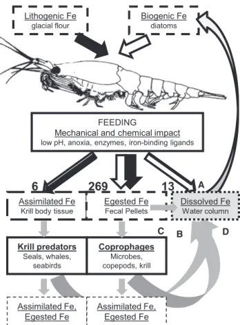
Our study shows that, on average, >90% of iron ingested by krill is re-packaged into fecal pellets rather than excreted as DFe or incorporated into body tissue (Figure 3). This is because iron concentrations in krill fecal pellets were 3–4 orders of magnitude higher than in muscle tissue and because >90%

of the iron released by krill during short-term incubations was in particulate rather than dissolved form. Therefore, the cycling of iron ingested by krill is closely linked to the fate of their fecal pellets. Even in the laboratory, sinking rates of krill fecal pellets are highly variable (1–51 m h ¹) depending on packaging den- C

B A

D

y = -0.0113x + 8.2375 R² = 0.5543

p = 0.001

6 7 8 9

Lithogenicparticles (log10µm3 stomach-1)

y = -48.09ln(x) + 240.64 R² = 0.413 p = 0.007

0 40 80 120 160

Fe in fecalpellets (µg mg-1dm)

y = -0.004ln(x) + 0.0237 R² = 0.5146 p = 0.021

0.000 0.005 0.010 0.015

Fe in muscle (µg mg-1dm)

y = -0.55ln(x) + 2.8703 R² = 0.6084 p = 0.003

0 2 4 6 8

0 50 100 150 200

Labile Fe (%TPFe)

Distance from glacial outlets (km) Pellets

PM

y = 3.591x - 25.07 R² = 0.6237

p = 0.011

0 1 2 3 4 5 6

6 7 8 9

DFeexcretion rate (nmolkrill-1d-1)

Diatoms (log10µm³stomach^-1)

y = 23.82x + 15.562 R² = 0.8711

p = 0.0001

0 40 80 120

0 1 2 3 4

TDFerelease rate (nmolkrill-1d-1)

Fecal pellets (mg dm)

E

F

Figure 2. Krill Iron Cycling

(A–D) Changes in krill characteristics with increasing distance from the major glacial outlet (Cumberland Bay).

(A) Volume of lithogenic particles in krill stomachs.

(B) Total particulate iron content in krill muscle tissue.

(C) Total particulate iron content in krill fecal pellets.

(D) Labile iron content in krill fecal pellets and in suspended particulate matter (PM) at 20 m water depth. Dm, dry mass; TPFe, total particulate iron.

(E and F) Results from nine short-term shipboard incubations of freshly caught krill.

(E) DFe excretion rates in relation to the volume of diatoms in krill stomachs.

(F) TDFe release rates in relation to the dry mass of fecal pellets produced during 3 hr incubations.

Table S1includes calculations of total DFe supply by krill.

sity, pellet volume, and mineral ballast [31]. In situ, pellet sinking is further modi- fied by turbulence and impact of grazers.

At several of our sampling stations, fecal pellets accounted for >70% of the suspended particulate matter in surface waters (Figure 1G), which suggests some retainment. While krill fecal pellets are traditionally seen as fast-sinking and exporting nutrients [32, 33], there is increasing awareness that a substantial proportion of pellets is fragmented and degraded in the upper ocean [34, 35], and nutrients are resupplied.

Regardless of the fate of these pellets, krill gut passage in- creases the proportion of labile iron and therefore the likelihood of subsequent iron dissolution due to photochemical reactions, ligand activity, microbial recycling, or zooplankton coprophagy [5, 35–37]. Radiotracer experiments have shown that 6–96 pM DFe d ¹can be released from copepod fecal pellets, which is similar in extent to iron regeneration from phytoplankton either due to viral lysis or grazing [37]. Thus, in addition to immediate DFe excretion by krill, further DFe may derive from the degradation of fecal pellets and the digestion of krill tissue by predators [37, 38]. In conclusion, krill uptake and mobilization of lithogenic and biogenic iron provides the basis for several pathways of DFe supply. These pathways involve the activity of other organisms—

microbes, zooplankton, krill predators—and abiotic processes (Figure 3), and in their sum they can deliver a substantial part of the phytoplankton iron demand.

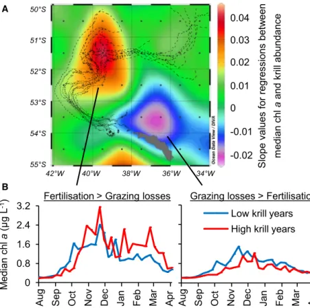
However, questions remain over the bioavailability of the supplied iron [39], the competition between bloom-forming diatoms and bacteria for iron [37], and the balance between phytoplankton fertilization and grazing losses [40]. Insights into the net effect of krill may be provided by the fact that krill abundances at South Georgia vary greatly from year to year due to far-field processes: the recruitment in their nursery grounds in the south and subsequent advection across the Scotia Sea [41]. High-krill years coincide with low chlaconcentrations on

(5)

the South Georgia shelf but high chlaconcentrations downstream (Figures 4A and 4B). In contrast, during low-krill years the bloom is shorter, less intensive, and lies closer to the island (Figure 2S). These correlations do not necessarily prove cause and effect, but may also reflect interannual variability in physical factors such as meltwater runoff, lateral advection of iron and macronutrients, or mixed-layer depth [43, 44]. However, the bloom downstream of South Georgia is clearly sourced by iron

supply from the island [12, 15, 44], so any process that enhances the concentration of DFe and TDFe in surface waters on the shelf would also contribute to the bloom development downstream.

At our outermost sampling station, the Fe:C ratios of diatom- dominated suspended matter were still 2 orders of magnitude higher (3600 ± 330mmol mol ¹) than values for diatoms under Fe-replete conditions elsewhere [45]. Luxury iron uptake by abundant pennate diatoms [46] on the shelf and their subsequent transport downstream may be an important mechanism for offshore iron fertilization, as it retains particulate iron and re- cycled iron in surface waters. The fact that, even in years with high krill grazing impact, the bloom was not entirely suppressed but rather was displaced beyond their habitat suggests that iron loss via sinking krill fecal pellets is secondary. In conclusion, we offer the hypothesis that long-lasting blooms downstream of South Georgia benefit from on-shelf iron mobilization and recycling by krill and other heterotrophs.

There is general consensus that zooplankton grazing is an important mechanism to recycle biogenic iron [28, 39]. This re- cycled iron seems to be highly bioavailable, as diatoms take up iron regenerated by copepods 43to 73faster than inorganic iron [39]. Copepods also release iron-binding ligands when grazing on phytoplankton [28, 29]. The ligands can complex with inorganic iron and thereby increase iron concentration solubility. Our study shows a third implication of zooplankton feeding: the mobilization of iron attached to lithogenic particles.

Acidic digestion and other gut processes can accelerate the dissolution of lithogenic iron, which is low in carbonate-buffered seawater. This mechanism was proposed based on enhanced trace-element mobility at lowered pH [6], but our field study now brings direct evidence. The ingestion of lithogenic particles is not restricted to Antarctic krill but is a widespread phenome- non among suspension-feeding zooplankton. It is known for copepods, mysids, salps, other euphausiids, and ciliates in river plums, fjords, at the seabed, or in the open ocean after dust deposition [47–53]. Therefore, iron mobilization by zooplankton could be important across a variety of habitats. Our study em- phasizes that ocean fertilization does not depend merely on physical iron supply but also on the prevailing foodweb structure that facilitates iron solubility, mobilization, and recycling.

EXPERIMENTAL PROCEDURES

This text summarizes the methods used, with theSupplemental Experimental Proceduresproviding full details.

Sampling

Our study took place during a research cruise at the northern shelf of South Georgia (Southern Ocean, 53–54S; 35–39W) from December 2010 to January 2011 onboard RRSJames Clark Ross. The station activities included (1) an acoustic survey to estimate local krill densities over the diurnal cycle, (2) live-krill sampling for stomach content analysis, fecal pellet production, iron measurements, and incubation experiments, (3) collection of suspended particulate matter by Stand-Alone Pump Systems (SAPS) for taxonomic identifi- cation and iron measurements, and (4) water sampling with towed fish and GO-FLO bottles for respective horizontal and vertical profiles of DFe and TDFe.

Krill Incubations

Under iron-clean conditions, freshly caught krill were rinsed and placed in 9L- polycarbonate carboys filled with 0.2mm filtered seawater from surface-towed trace metal clean fish. At each station, two to three replicate carboys each Lithogenic Fe

glacial flour

Biogenic Fe diatoms

FEEDING

Mechanical and chemical impact low pH, anoxia, enzymes, iron-binding ligands

Assimilated Fe Krill body tissue

Egested Fe Fecal Pellets

Krill predators Seals, whales,

seabirds

Coprophages Microbes, copepods, krill

A

C B

Assimilated Fe, Egested Fe

D

6 269 13

Assimilated Fe, Egested Fe

Dissolved Fe Water column

Figure 3. Schema of Iron Flux through Krill and Pathways of DFe Supply

The numbers (nmol Fe g¹krill dm d ¹) indicate the partitioning of ingested iron between body tissue, fecal pellets and the ambient pool of dissolved iron (details are given inTable S2). On a daily basis,5% of the krill body iron content is assimilated, >200% is egested via fecal pellets, and10% is directly excreted as DFe. This indicates the high iron content of the ingested food compared to krill’s own requirements. The iron that is ingested and mobilized by krill can reach the DFe pool via several pathways (indicated in A–D).

(A) Direct excretion by krill.

(B) Release from krill fecal pellets due to microbial degradation and zooplankton coprophagy.

(C) Release from krill fecal pellets due to the dissolution of particulate iron via complexation with ligands or photochemical reactions.

(D) Digestion of krill tissue by predators.

All of these processes can occur in the upper mixed layer but may also happen in deeper water due to krill vertical migration and the sinking of their pellets.

Black and open arrows represent the relative fractions sourced from lithogenic and biogenic iron, respectively. Gray arrows indicate processes that remain to be quantified. InTable S3, DFe fluxes from krill are compared to those from physical sources.

2670 Current Biology26, 2667–2673, October 10, 2016

(6)

containing 10–20 krill and two control carboys without krill were run at 2C. The incubation water was sampled for DFe and TDFe initially and after 1 hr and 3 hr.

At termination of the experiment, the remaining fecal pellets were collected for dry mass estimates.

Iron Measurements

In a trace metal clean laboratory container onboard the ship, water samples for DFe (<0.2mm) and TDFe (unfiltered) were acidified with ultra-pure HNO3to pH 1.66 for subsequent analysis by inductively coupled plasma-mass spectrom- etry (ICP-MS). The labile particulate iron fraction was remobilized with a 25%

acetic acid solution at room temperature for 3 hr. The refractory particulate iron was digested in a mixture of concentrated HNO3, HCl, and HF acids at 140C for 4 hr. Both labile and refractory particulate iron were analyzed by ICP-MS.

SUPPLEMENTAL INFORMATION

Supplemental Information includes Supplemental Experimental Procedures, two figures, and three tables and can be found with this article online at http://dx.doi.org/10.1016/j.cub.2016.07.058.

AUTHOR CONTRIBUTIONS

Conceptualization, K.S., A.A., and E.P.A.; Methodology, C.S., A.A., S.F., and K.S.; Investigation, C.S., A.A., K.S., S.F., H.J.V., and C.M.W.; Writing – Original Draft, K.S.; Writing – Review & Editing, K.S., A.A., E.P.A., and C.S.; Funding Acquisition, A.A., E.P.A., and K.S.

ACKNOWLEDGMENTS

We thank the officers, crew, and scientists onboard the RRSJames Clark Ross for their professional support during JR247 and M. Patey for the SAPS deploy- ment. E. Bazeley-White and H. Peat helped with the acquisition of data from BAS and NERC databases, and M. Meredith supplied the drifter data. We acknowledge the MODIS mission scientists and associated NASA personnel

for the production of data in the Giovanni online data system. We are grateful to E. Young, M. Lohan, V. Kitidis, and D. Bakker for discussing our results.

Comments from V. Smetacek and two anonymous reviewers greatly improved the work. This study was funded by the UK Natural Environment Research Council grant NE/F01547X/1. A.A. was additionally funded by NERC and Department for Environment, Food and Rural Affairs (DEFRA) grant NE/L 003279/1 (Marine Ecosystems Research Program).

Received: June 10, 2016 Revised: July 19, 2016 Accepted: July 22, 2016 Published: September 15, 2016 REFERENCES

1.Martin, J.H. (1990). Glacial-interglacial CO2change: the iron hypothesis.

Paleoceanography5, 1–13.

2.Moore, C.M., Mills, M.M., Arrigo, K.R., Berman-Frank, I., Bopp, L., Boyd, P.W., Galbraith, E.D., Geider, R.J., Guieu, C., Jaccard, S.L., et al. (2013).

Processes and patterns of oceanic nutrient limitation. Nat. Geosci.6, 701–710.

3.Buck, K.N., Lohan, M.C., Berger, C.J.M., and Bruland, K.W. (2007).

Dissolved iron speciation in two distinct river plumes and an estuary:

implications for riverine iron supply. Limnol. Oceanogr.52, 843–855.

4.Raiswell, R., Tranter, M., Benning, L.G., Siegert, M., De’ath, R., Huybrechts, P., and Payne, T. (2006). Contributions from glacially derived sediment to the global iron (oxyhydr)oxide cycle: Implications for iron delivery to the oceans. Geochim. Cosmochim. Acta70, 2765–2780.

5.Baker, A.R., and Croot, P.L. (2010). Atmospheric and marine controls on aerosol iron solubility in seawater. Mar. Chem.120, 4–13.

6.Moore, R.M., Milley, J.E., and Chatt, A. (1984). The potential for biological mobilization of trace elements from aeolian dust and its importance in the case of iron. Oceanol. Acta7, 221–228.

Slope values for regressions between median chlaand krill abundance

42°W 40°W 38°W 36°W 34°W 50°S

51°S

52°S

53°S

54°S

55°S

0.04 0.03 0.02 0.01 0 -0.01 -0.02 A

Median chla(μg L-1) 0 0.8 1.6 2.4

3.2

Years with …

Grazing losses > Fertilisation Fertilisation > Grazing losses

Low krill years High krill years B

Aug Sep Oct Nov Dec Jan Feb Mar Apr Aug Sep Oct Nov Dec Jan Feb Mar Apr

Figure 4. The Potential Role of Krill in Phyto- plankton Fertilization and Grazing Losses (A) Spatial distribution of negative (blue-purple) and positive (yellow-red) slope values for the regression between median chlaconcentration and summer krill abundance on the South Georgia shelf for the years 2002–2013 (details inFigure S2). Chlaconcentrations were derived from ocean color radiometry (MODIS 2002–2013, mid-August to mid-April, 8-day composites). The black lines are drifter trajectories that indicate that surface currents link the northern shelf of South Georgia to the main bloom area downstream, with a transit time of 20–50 days [42].

(B) The time course of the average annual chl a development downstream of South Georgia (yellow- red area in A) and on the shelf (blue-purple area in A) during high- and low-krill years. The left plot indicates that the blooms downstream extend into autumn when the krill abundance on the shelf is high, but they are restricted to spring and summer when the krill abundance is low. In the area that benefits most from fertilization, the median chlaconcentration increased from 1.0 to 1.3mg L ¹and the bloom duration from 12 to 16 weeks in high-krill years. A bloom was defined asR1mg chlaL ¹. Low-krill years at South Georgia:

2002/2003, 2003/2004, 2004/2005, 2008/2009, 2010/

2011, 2012/2013. High-krill years: 2005/2006, 2007/

2008, 2009/2010, 2011/2012.

(7)

7.Gordon, J.E., Haynes, V.M., and Hubbard, A. (2008). Recent glacier changes and climate trends on South Georgia. Global Planet. Change 60, 72–84.

8.D’Odorico, P., Bhattachan, A., Davis, K.F., Ravi, S., and Runyan, C.W. (2013).

Global desertification: Drivers and feedbacks. Adv. Water Resources51, 326–344.

9.Barker, A.J., Douglas, T.A., Jacobson, A.D., McClelland, J.W., Ilgen, A.G., Khosh, M.S., Lehn, G.O., and Trainor, T.P. (2014). Late season mobilisation of trace metals in two small Alaskan arctic watersheds as a proxy for land- scape scale permafrost active layer dynamics. Chem. Geol.381, 180–193.

10. Gutt, J., Bertler, N., Bracegirdle, T.J., Buschmann, A., Comiso, J., Hosie, G., Isla, E., Schloss, I.R., Smith, C.R., Tournadre, J., et al. (2014). The Southern Ocean ecosystem under multiple climate change stresses – an integrated circumpolar assessment. Glob. Change Biol. http://dx.doi.

org/10.1111/gcb.12794.

11.de Baar, H.J.W., de Jong, J.T.M., Bakker, D.C.E., Lo¨scher, B.M., Veth, C., Bathmann, U., and Smetacek, V. (1995). Importance of iron for plankton blooms and carbon dioxide drawdown in the Southern Ocean. Nature 373, 412–415.

12.Korb, R.E., Whitehouse, M.J., and Ward, P. (2004). SeaWiFS in the southern ocean: spatial and temporal variability in phytoplankton biomass around South Georgia. Deep Sea Res. Part II Top. Stud. Oceanogr.51, 99–116.

13.Blain, S., Que´guiner, B., Armand, L., Belviso, S., Bombled, B., Bopp, L., Bowie, A., Brunet, C., Brussaard, C., Carlotti, F., et al. (2007). Effect of natural iron fertilization on carbon sequestration in the Southern Ocean.

Nature446, 1070–1074.

14.Planquette, H., Statham, P.J., Fones, G.R., Charette, M.A., Moore, C.M., Salter, I., Ne´de´lec, F.H., Taylor, S.L., French, M., Baker, A.R., et al.

(2007). Dissolved iron in the vicinity of the Crozet Islands, Southern Ocean. Deep Sea Res. Part II54, 1999–2019.

15.Nielsdo´ttir, M.C., Bibby, T.S., Moore, C.M., Hinz, D.J., Sanders, R., Whitehouse, M., Korb, R., and Achterberg, E.P. (2012). Seasonal and spatial dynamics of iron availability in the Scotia Sea. Mar. Chem.130- 131, 62–72.

16.Gerringa, L.J.A., Alderkamp, A.-C., Laan, P., Thuro´czy, C.-E., de Baar, H.J.W., Mills, M.M., van Dijken, G.L., van Haren, H., and Arrigo, K.R.

(2012). Iron from melting glaciers fuels the phytoplankton blooms in Amundsen Sea (Southern Ocean): Iron biogeochemistry. Deep Sea Res.

Part II71, 16–31.

17. Hawkings, J.R., Wadham, J.L., Tranter, M., Raiswell, R., Benning, L.G., Statham, P.J., Tedstone, A., Nienow, P., Lee, K., and Telling, J. (2014). Ice sheets as a significant source of highly reactive nanoparticulate iron to the oceans. Nat. Commun.5, 3929.http://dx.doi.org/10.1038/ncomms4929.

18. Hopwood, M.J., Statham, P.J., Tranter, M., and Wadham, J.L. (2014).

Glacial flour as a potential source of Fe(II) and Fe(III) to polar waters.

Biogeochemistry118, 443–452.http://dx.doi.org/10.1007/s10533-013- 9945-y.

19.Schroth, A.W., Crusius, J., Hoyer, I., and Campbell, R. (2014). Estuarine removal of glacial iron and implications for iron fluxes to the ocean.

Geophys. Res. Lett.41, 3951–3958.

20.Zhang, R.F., John, S.G., Zhang, J., Ren, J.L., Wu, Y., Zhu, Z.Y., Liu, S.M., Zhu, X.C., Marsay, C.M., and Wenger, F. (2015). Transport and reaction of iron and iron stable isotopes in glacial meltwaters on Svalbard near Kongsfjorden: From rivers to estuary to ocean. Earth Planet. Sci. Lett.

424, 201–211.

21.Atkinson, A., Whitehouse, M.J., Priddle, J., Cripps, G.C., Ward, P., and Bandon, M.A. (2001). South Georgia, Antarctica: a productive, cold water, pelagic ecosystem. Mar. Ecol. Prog. Ser.216, 279–308.

22.Syvitski, J.P.M., and Lewis, A.G. (1980). Sediment ingestion byTigriopus californicusand other zooplankton: mineral transformation and sedimen- tological considerations. J. Sediment. Petrol.50, 869–880.

23.Engelhardt, H.J., and Brockamp, O. (1995). Biodegradation of clay-min- erals – laboratory experiments and results from Wadden Sea tidal flat sed- iments. Sedimentology42, 947–955.

24.Needham, S.J., Worden, R.H., and McIlroy, D. (2004). Animal-sediment in- teractions: the effect of ingestion and excretion by worms on mineralogy.

Biogeosci.1, 113–121.

25.Dall, W., and Moriarty, D.J.W. (1983). Functional aspects of nutrition and digestion. In The biology of crustaceans,Volume 5, L.H. Mantel, ed.

(Academic Press), pp. 215–261.

26.Tang, K.W., Glud, R.N., Glud, A., Rysgaard, S., and Nielsen, T.G. (2011).

Copepod guts as biogeochemical hotspots in the sea: Evidence from microelectrode profiling ofCalanusspp. Limnol. Oceanogr.56, 666–672.

27.Liu, X., and Millero, F.J. (2002). The solubility of iron in seawater. Mar.

Chem.77, 43–54.

28.Hutchins, D., Witter, A., Butler, A., and Luther, G. (1999). Competition among marine phytoplankton for different chelated iron species. Nature 400, 858–861.

29.Sato, M., Takeda, S., and Furuya, K. (2007). Iron regeneration and organic iron(III)-binding ligand production during in situ zooplankton grazing experiment. Mar. Chem.106, 471–488.

30. Tovar-Sańchez, A., Duarte, C.M., Hernańdez-Leoń, S., and San˜udo- Wilhelmy, S.A. (2007). Krill as a central node for iron cycling in the Southern Ocean. Geophys. Res. Lett.34, L11601.http://dx.doi.org/10.

1029/2006GL029096.

31.Atkinson, A., Schmidt, K., Fielding, S., Kawaguchi, S., and Geissler, P.

(2012). Variable food absorption by Antarctic krill: relationship between diet, egestion rate and the composition and sinking rates of their fecal pellets. Deep Sea Res. Part II Top. Stud. Oceanogr.59-60, 147–158.

32.von Bodungen, B., Fischer, G., No¨thig, E.-M., and Wefer, G. (1987).

Sedimentation of krill faeces during spring development of phytoplankton in Bransfield Strait, Antarctica. Mitt. Geol. Pal€aontol. Inst. Uni. Leipzig62, 243–257.

33.Manno, C., Stowasser, G., Enderlein, P., Fielding, S., and Tarling, G.A.

(2015). The contribution of zooplankton faecal pellets to deep carbon transport in the Scotia Sea (Southern Ocean). Biogeosci. Discuss.11, 16105–16134.

34.Gonza´lez, H.E. (1992). The distribution and abundance of krill faecal material and oval pellets in the Scotia Sea and Weddell Seas (Antarctica) and their role in particle flux. Polar Biol.12, 81–91.

35. Belcher, A., Iversen, M., Manno, C., Henson, S.A., Tarling, G.A., and Sanders, R. (2016). The role of particle associated microbes in remineral- ization of fecal pellets in the upper mesopelagic of the Scotia Sea, Antarctica. Limnol. Oceanogr.61,http://dx.doi.org/10.1002/lno.10269.

36.Borer, P.M., Sulzberger, B., Reichard, P., and Kraemer, S.M. (2005). Effect of siderophores on the light-induced dissolution of colloidal iron(III) (hydr) oxides. Mar. Chem.93, 179–193.

37.Boyd, P.W., Strzepek, R., Chiswell, S., Chang, H., DeBruyn, J.M., Ellwood, M., Keenan, S., King, A.L., Maas, E.W., Nodder, S., et al. (2012). Microbial control of diatom bloom dynamics in the open ocean. Geophys. Res. Lett.

39, L18601.

38.Nicol, S., Bowie, A., Jarman, S., Lannuzel, D., Meiners, K.M., and van der Merwe, P. (2010). Southern Ocean iron fertilization by baleen whales and Antarctic krill. Fish Fish.11, 203–209.

39.Nuester, J., Shema, S., Vermont, A., Fields, D.M., and Twining, B.S. (2014).

The regeneration of highly bioavailable iron by meso- and microzooplankton. Limnol. Oceanogr.59, 1399–1409.

40.Whitehouse, M.J., Atkinson, A., Ward, P., Korb, R.E., Rothery, P., and Fielding, S. (2009). Role of krill versus bottom-up factors in controlling phytoplankton biomass in the northern Antarctic waters of South Georgia. Mar. Ecol. Prog. Ser.393, 69–82.

41. Murphy, E.J., Trathan, P.N., Watkins, J.L., Reid, K., Meredith, M.P., Forcada, J., Thorpe, S.E., Johnston, N.M., and Rothery, P. (2007).

Climatically driven fluctuations in Southern Ocean ecosystems. Proc.

Biol. Sci.274, 3057–3067.http://dx.doi.org/10.1098/rspb.2007.1180.

42. Meredith, M.P., Watkins, J.L., Murphy, E.J., Cunningham, N.J., Wood, A.G., Korb, R., Whitehouse, M.J., and Thorpe, S.E. (2003). An anticyclonic 2672 Current Biology26, 2667–2673, October 10, 2016

(8)

circulation above the Northwest Georgia Rise, Southern Ocean. Geophys.

Res. Lett.30, 2061.http://dx.doi.org/10.1029/2003GL018039.

43.Young, E.F., Thorpe, S.E., Banglawala, N., and Murphy, E.J. (2014).

Variability in transport pathways on and around the South Georgia shelf, Southern Ocean: Implications for recruitment and retention. J. Geophys.

Res. Oceans119, 241–252.

44. Robinson, J., Popova, E.E., Srokosz, M.A., and Yool, A. (2016). A tale of three islands: Downstream natural iron fertilization in the Southern Ocean. J. Geophys. Res. Oceans 121, http://dx.doi.org/10.1002/

2015JC011319.

45.Twining, B.S., Baines, S.B., Fisher, N.S., and Landry, M.R. (2004). Cellular iron contents of plankton during the Southern Ocean Iron Experiment (SOFeX). Deep Sea Res. Part I Oceanogr. Res. Pap.51, 1827–1850.

46.Marchetti, A., Parker, M.S., Moccia, L.P., Lin, E.O., Arrieta, A.L., Ribalet, F., Murphy, M.E.P., Maldonado, M.T., and Armbrust, E.V. (2009). Ferritin is used for iron storage in bloom-forming marine pennate diatoms.

Nature457, 467–470.

47.Tackx, M.L.M., Herman, P.J.M., Gasparini, S., Irigoien, X., Billiones, R., and Daro, M.H. (2003). Selective feeding of Eurytemora affinis (Copepoda, Calanoida) in temperate estuaries: model and field observa- tions. Estuar. Coast. Shelf Sci.56, 305–311.

48.Arendt, K.E., Dutz, J., Jo´nasdo´ttir, S.H., Jung-Madsen, S., Mortensen, J., Møller, E.F., and Nielsen, T.G. (2011). Effects of suspended sediment on copepods feeding in a glacial influenced sub-Arctic fjord. J. Plankton Res.33, 1526–1537.

49.Song, K.H., and Breslin, V.T. (1999). Accumulation and transport of sediment metals by vertically migrating opossum shrimp,Mysis relicta.

J. Great Lakes Res.25, 429–442.

50.Pakhomov, E.A., Fuentes, V., Schloss, I., Atencio, A., and Esnal, G.B.

(2003). Beaching of the tunicateSalpa thompsoniat high levels of suspended particulate matter in the Southern Ocean. Polar Biol.26, 427–431.

51.Schmidt, K. (2010). Food and feeding in Northern krill (Meganyctiphanes norvegicaSars). Adv. Mar. Biol.57, 127–171.

52.Schmidt, K., Atkinson, A., Steigenberger, S., Fielding, S., Lindsay, M.C.M., Pond, D.W., Tarling, G., Klevjer, T.A., Allen, C.S., Nicol, S., et al. (2011).

Seabed foraging by Antarctic krill: implications for stock assessment, ben- tho-pelagic coupling and the vertical transfer of iron. Limnol. Oceanogr.

56, 1411–1428.

53.Boenigk, J., and Novarino, G. (2004). Effect of suspended clay on the feeding and growth of bacterivorous flagellates and ciliates. Aquat.

Microb. Ecol.34, 181–192.

(9)

Current Biology, Volume26

Supplemental Information

Zooplankton Gut Passage Mobilizes Lithogenic Iron for Ocean Productivity

Katrin Schmidt, Christian Schlosser, Angus Atkinson, Sophie Fielding, Hugh J.

Venables, Claire M. Waluda, and Eric P. Achterberg

(10)

y = -1038.4x + 35131 R² = 0.6886

p = 0.0001

0 50 100 150 200 250 300 350 400

33.5 33.6 33.7 33.8 33.9

TDFe (nM)

Salinity y = -29.892x + 1011.5

R² = 0.7091 p = 0.0001

0 1 2 3 4 5 6 7 8 9 10

33.5 33.6 33.7 33.8 33.9

DFe (nM)

Salinity Fish

GoFlo

A

DFe (nmol L^-1)

CB

53°S

54°S

55°S

10 8 6 4 2 0

TDFe (nmol L^-1)

400 300 200 100

0 Chlorophyll a (µg L^-1)

3.5 3 2.5 2 1.5 1 0.5 Salinity

39°W 38°W 37°W 36°W

33.8

33.6

33.4

33.2

53°S

54°S

55°S

B

39°W 38°W 37°W 36°W

Fig. S1, Related to Fig. 1. Dissolved and total dissolvable iron concentrations north of South Georgia (study period: 25^th Dec 2010 – 19^th Jan 2011).

A, Concentrations of dissolved iron (< 0.2 µm, DFe) and total dissolvable iron (unfiltered, TDFe), salinity and chlorophyll a in surface waters from major glacial outlets at Cumberland Bay (CB) across the northern shelf and downstream of the island. B, Relationship between DFe- and TDFe concentration and salinity in surface waters (‘Fish’, station locations in Fig. S1A) or at 20 m water depth (‘GoFlo’, station locations to the right).

(11)

Fig. S2, Related to Fig. 4. Annual differences in bloom intensity and duration

Average chl a concenration (A) and bloom duration (B) in years with low (left) and high (right) krill abundances on the South Georgia shelf.

Low krill years at South Georgia: 2002/3, 2003/4, 2004/5, 2008/9, 2010/2011, 2012/2013. High krill years: 2005/6, 2007/8, 2009/10, 2011/2012.

Chl a concentrations were derived from ocean colour radiometry (MODIS 2002-2013, mid August-mid April, 8-day composites). A bloom was defined as ≥1 µg Chl a L^-1. Years of high krill abundance

Years of low krill abundance

A

B

Median chla (µg L-1) 1

0.8

0.6

0.4

0.2

Bloom duration (weeks)

20

15

10

5

0

(12)

DFe-demand by phytoplankton DFe-supply by krill Percentage

Event Chl a PP DFe-demand-A UML DFe-demand-B DFe excretion No krill-A DFe supply-A No krill-B DFe supply-B % % (mg m^-3) (g C m^-2 d^-1) (µmol Fe m^-2 d^-1) (m) (nmol Fe m^-3 d^-1) (nmol Fe ind^-1d^-1) (ind m^-2) (µmol Fe m^-2 d^-1) (ind m^-3) (nmol Fe m^-3 d^-1)

17 2 0.46 1.43 60 23.8 5.3 185 0.98 1.4 7.4 69 31

44 1.3 0.36 1.12 60 18.6 1.1 185 0.2 1.4 1.5 18 8

67 1.5 0.39 1.21 60 20.1 3.3 130 0.43 0.9 3.0 35 15

92 0.26 0.21 0.65 70 9.4 4.3 1582 6.88 7.1 31 1050 331

107 0.26 0.21 0.65 70 9.4 0.1 1408 0.21 6.3 0.9 32 10

116 0.35 0.23 0.69 45 15.4 2.3 264 0.61 1.4 3.2 87 21

128 0.35 0.23 0.69 45 15.4 1.1 194 0.2 1.0 1.1 29 7

145 0.7 0.28 0.85 60 14.2 0.4 172 0.08 1.0 0.5 9 3

154 1 0.32 0.98 60 16.4 0.2 61 0.02 0.5 0.1 2 1

Mean 0.9 0.3 0.9 59 15.9 2.0 464 1.1 2.3 5.4

Table S1, Related to Figure 2. Comparison between phytoplankton DFe demand and krill DFe supply for stations where the release of DFe by krill had been measured in ship-board incubations. blue – rates are expressed as per m^-2 for the upper ~300 m water column, red – rates are expressed as per m^-3for the upper mixed layer (UML), green – results from ship-board incubations of krill.

Assumptions: (1) PP at South Georgia can be calculated from Chl a values using the equation y = 144.59 x + 174.77, R² = 0.8322 (original data in [S1]).

(2) A Fe:C ratio of 37 µmol mol^-1 is representative for natural phytoplankton populations under Fe-replete conditions [S2].

Krill density (g m^-2) and their vertical distribution across day- and night-time were estimated from acoustic backscattering. Average krill dry mass varied from 0.1 to 0.22 g ind^-1 between stations.

Calculations:

DFe-demand-A (µmol Fe m^-2 d^-1) = Primary production (PP, g C m^-2 d^-1) × Fe:C ratio (µmol mol^-1) DFe-demand-B (nmol Fe m^-3 d^-1) = DFe-demand-A (µmol Fe m^-2 d^-1) × 1000/ UML depth (m) No of krill-A (ind m^-2) = krill density (g m^-2) in upper 300 m water column/ krill dry mass (g ind^-1) No of krill-B (ind m^-3) = No of krill-A (ind m^-2) * percentage of krill in UML/ UML depth (m) DFe-supply-A (µmol Fe m^-2 d^-1) = DFe-excretion rate (nmol Fe ind^-1 d^-1) × No of krill-A (ind m^-2) DFe-supply-B (nmol Fe m^-3 d^-1) = DFe-excretion rate (nmol Fe ind^-1 d^-1) × No of krill-B (ind m^-3)

(13)

Iron cycling through krill DFe supply from zooplankton feeding Particulate Fe (PFe) Dissolved Fe (DFe) (DFe release rate × biomass)

 PFe in tissue  DFe release from tissue 0.6-2.8 pM d^-1 (copepods, [S7])

Muscle: 4-13 µg Fe g^-1dm[this study], [S3] unknown 0.7-5.8 pM d^-1 (mixed mesozooplankton, [S8]) Stomach: 0.03- 6 mg Fe g^-1dm[S3] 0.8-8 pM d^-1 (micro- and mesozooplankton, [S9]) Whole krill: 4-174 µg Fe g^-1 dm [S4], [S5] 0.1 – 31 pM d^-1(krill, [this study])

 PFe in fecal pellets  DFe release from pellets 31 pM d^-1 (microzooplankton, [S10]) 2-149 mg Fe g^-1dm[this study] unknown 17-115 pM d^-1(microzooplankton, [S11])  TDFe release when feeding  DFe release when feeding

0.02-0.6 µmol TDFe g^-1dm d^-1 [this study] 0.9-34 nmol DFe g^-1 dm d^-1 (this study) DFe supply from fecal pellets

0.5-16.5 µmol TDFe g^-1 dm d^-1 [S6] 6-96 pM d^-1 (copepods, [S11])

Table S2, Related to Figure 3. Overview of iron measurements in krill tissue, fecal pellets and incubation water, and DFe supply from zooplankton feeding

Calculation of TDFe- and DFe release rates were based on a krill dry mass (dm) of 0.156 g ind^-1, which represents an average value for the sampling stations of this study.

(14)

Location Source DFe flux (µmol m^-2 d^-1) Reference South Georgia Krill grazing (upper mixed layer) 0.35 (range 0.006-2.2) This study Krill grazing (upper 300 m) 1.1 (range 0.02-6.9) This study

Kerguelen region Atmospheric dust 0.05 ± 0.039 [S12]

Kerguelen plateau Upwelling 0.2 – 0.25 [S12]

Kerguelen plume Upwelling 0.14-0.33 [S12]

Kerguelen plateau Diffusion 0.042-0.093 [S12]

Kerguelen plume Diffusion 0.0005-0.001 [S12]

Pine Island Glacier Lateral diffusion (incl. phytopl. uptake) 66 at 40 km from source [S13]

31 at 70 km from source 3.1 at 159 km from source Table S3, Related to Figure 3. Fluxes of DFe from krill and physical sources.

Note: To our knowledge there are no data from physical sources available for South Georgia.. Therefore we used estimates from the Kerguelen Region, which is to some extent similar to South Georgia (but without Antarctic krill and less glacial run-off). The Pine Island Glacier in the Amundsen Sea is much larger than glaciers at South Georgia and a very important iron source to the region.

(15)

Supplemental Experimental Procedures

Cruise details. This study was part of a research expedition to the northern shelf of South Georgia from 25^th December 2010 to 19^th January 2011 onboard RRS James Clark Ross.

Temperature, salinity and fluorescence. Vertical profiles of conductivity-temperature-depth (CTD) and fluorescence were collected with a SeaBird Electronics 9 Plus (SBE 9Plus) CTD and attached Aqua Tracka fluorometer (Chelsea Instruments). Underway surface salinity and fluorescence were obtained from the Oceanlogger SBE45 CTD using the ship’s seawater supply. Non-calibrated fluorescence data are given in ‘relative units’.

Abundance of diatom, flagellates, ciliates and bacteria . At each station, discrete water samples for taxonomic analysis of the plankton community were taken from 20m depth with a 10L Niskin bottle on a standard stainless steel CTD rosette. Samples were preserved with 2% acidic Lugol’s solution and stored in 250 ml amber glass bottles. A 50 ml sub-sample was settled for 24h in an Utermöhl counting receptacle and examined with an inverted microscope (Zeiss, Axiovert 25). Rare items (i.e. large diatoms, thecate dinoflagellates and large ciliates) were counted by scanning the complete receptacle at × 200

magnification, while small common items were enumerated from two perpendicular transects across the whole diameter of the receptacle. The smallest items included in this study were approximately 5 µm. Autotrophic flagellates, small naked dinoflagellates and thecate dinoflagellates were grouped as ‘flagellates’.

The dimensions of the different taxa were measured and the volume calculated based on simple geometric shapes or combinations thereof [S14].

Composition of suspended particulate matter. Stand-Alone Pumping Systems (SAPS, Challenger Oceanic) were deployed to sample suspended particulate matter from 20m, 50m and 150m water depth. Material was pumped for 1-1.5 hours and filtered onto polycarbonate filters (293 mm diameter, 1 µm pore-size, Sterlitech, USA). From each filter a small piece (~5 cm²) was cut out with a ceramic knife for subsequent microscopical examination. The remaining filter was stored at -20°C for trace metal analysis. The microscopical analysis was carried out in analogue to that of plankton samples obtained with the Niskin bottles.

However, due to the larger volume (mean: 530±210 L) and greater water depth, SAPs samples contained additional items such as copepods, nauplii, pteropods, tintinnids, fecal pellets and lithogenic particles. All items were enumerated and their dimensions measured. The volume and carbon content of copepods was estimated from their prosome length, that of nauplii from the total length according to [S15]. The shape of other items was considered to be either spherical (pteropods, some fecal pellets), cylindrical (fecal pellets) or a truncated cone (tintinnids). Due to intermediate size or breakage, fecal material (≥ 25 µm diameter) was combined into one category regardless its origin from copepods, euphausiids or pteropods. Lithogenic particles were counted in 3 size fractions: 5-10 µm, 11-25 µm and 26-50 µm and the volume was considered to be equal to a half-sphere.

Krill acoustics. Krill density (g m^-2) and their vertical distribution were estimated from acoustic backscattering according to [S16]. The mean krill density per station was calculated from multiple 10-nm-transects across the area. Usually 5-7 transects were run to span a diel cycle. By pooling day-time vs. night-time transects, patterns in krill diurnal vertical migration were extracted. For the conversion of krill density (g m^-2) into carbon concentrations (mg C m^-3), first, the average wet mass of krill in the upper 50 m water column was calculated using day- and night-time vertical distribution profiles and, second, wet mass was transferred into carbon content applying a multiplication factor of 0.0993 [S17].

Live krill sampling was based on targets identified with the echosounder and carried out with purpose-built 1 m² square nets. To allow for short duration hauls, all but one of the targets were in the upper 50 m water column. Solid plastic cod ends minimised abrasion to the catch. Onboard, krill were immediately

transferred into the cold room (2°C). A batch of ~50 krill was frozen at -80°C for diet analysis and trace metal analysis of muscle tissue.

Krill stomach content. To examine krill diet, the stomach was dissected from frozen krill and samples were analysed according to [S3],[S14].

Fecal pellet collection. About 150-200 healthy individuals were sequentially washed in a series of acid-cleaned buckets filled with 0.2 µm-filtered seawater obtained from trace metal clean towed fish and then left for defecation in a laminar flow cabinet in a temperature-controlled room (2°C). Fecal pellets were collected at 0.5-1 h intervals over a maximum of 3 hours using acid washed plastic pipettes. The pellets were purified, transferred to an acid washed plastic tube, rinsed twice with deionised water (Milli-Q, Millipore) and then frozen at -80°C for subsequent analysis of trace metals.