Assessing a 6C Kalman filter using experimental datasets from an industrial robot

(1)

Conference Poster

Assessing a 6C Kalman filter using experimental datasets from an industrial robot

Author(s):

Rossi, Yara; Tatsis, Konstantinos; Arbogast, Konstantin; Awadaljeed, Mudathir; Chatzi, Eleni; Rothacher, Markus; Clinton, John Francis

Publication Date:

2020-12

Permanent Link:

https://doi.org/10.3929/ethz-b-000460164

Rights / License:

In Copyright - Non-Commercial Use Permitted

(2)

https://agu2020fallmeeting-agu.ipostersessions.com/Default.aspx?s=B7-F7-3C-23-70-CA-3E-13-83-40-08-0A-F6-4E-B0-C1&pdfprint=true&gues… 1/17

Assessing a 6C Kalman Filter using

Experimental Datasets from an Industrial Robot

Yara Rossi, Konstantinos Tatsis, Mudathir Awadaljeed, Konstantin Arbogast, Eleni Chatzi, Markus Rothacher, John Clinton

Institut of Geodesy and Photogrammetrie, Swiss Seismological Service, Institute of Structural Engineering, ETH Zurich

PRESENTED AT:

(3)

1. MOTIVATION

Figure 1: The influence rotation has on the three instruments IMU, accelerometer and GNSS antenna (from left to right).

Adapted from Lin et al., 2010.

Many monitoring stations are nowadays equipped with inertial seismometers for weak motions, accelerometers for strong motions and - more recently - even GNSS antennas and receivers that directly measure displacement. Combined, these 3 sensors allow for the recording of an extremely broad range of seismic motion. However, these instruments only measure the 3 translational components, but can be influenced by rotations occurring simultaneously (see Figure 1). We address this issue by adding an instrument to the monitoring station, which can directly record rotations as has been proposed by Farrell, 1969 and Graizer, 1991. In this study a high quality inertial measurement unit (IMU) was used to record the angular velocity additional to an EpiSensor and Centaur digitizer recording acceleration and a Javad antenna and Septentrio receiver recording displacement.

(4)

2. EXPERIMENT SETUP

[VIDEO] https://player.vimeo.com/video/480782807?byline=0&badge=0&portrait=0&title=0

(5)

The experimental set up consists of three measuring instruments and a six-axis industrial robot arm performing the 6C ground motions.

The generated 6C groundmotions simulate the top of a windturbine with motion in and about the horizontal axis. The vertical component is not provided with any motion. Nonetheless, high frequency 'ticks' are visible on and about the vertical axis due to axis rotation changes within the robot arm seen in Figure 4 and 5 in Section 6.

The video above shows the motion during the experiment with the largest motion TLRL (see Figure 2). The GNSS antenna as well as the IMU are simultaneously attached to a platform atop the robot arm (see video) and the accelerometer is mounted at a different time and the experiments are performed twice.

Three experiment sets:

300 s time series Tz, Rz no motion Tx ∝ Ry and Ty ∝ Rx 3 periods longer than 100 s 3 - 5 periods around 3 s

Figure 2: The relative amplitudes of the three experiments. The naming is designed to facilitate comprehension for the reader. T: translation, R: rotation, L: large, S: small.

(6)

3. ROBOT REPEATABILITY

Since we are using the robot feedback as a ground truth for the accomplished motion and therefore as a reference for comparing the KF estimates, it is important to determine the quality and repeatability of these signals. This was analysed by comparing the four repetitions of one experiment among each other and calculating the RMS of the discrepancies (error) in terms of the translations and rotations.

for N = length of signal

Figure 3: Mean RMSE of the difference between the robot feedback of different repetitions of the same experiment for translations and rotations of each experiment TLRL, TLRS, TSRS.

RMSEmean= ∑¹₆ ³_i=1∑⁴_j=i+1√∑^N_n=0 (expj−expi)2n N

(7)

4. 6C KALMAN FILTER (KF)

State Equation

Observation Equation

The methodology chosen for the combination of the three instruments is the standard sensor fusion linear Kalman filter (KF). An advantage is the ability of combining diverse instruments, measuring different quantities and at different sampling rates. Two pre-computations are executed prior to the filter itself, namely the integration of the angular velocity and the rotation of the acceleration recordings into the local coordinate system.

The state (process) equation of the KF is designed using the standard adoption of displacement and velocity in the state vector x. The pre-rotated accelerations a and the rotation of the vector h (antenna phase center offset from the point of rotation on the robot), serve for formulating the KF input vector u.

x_k=

⎡⎢

⎢ ⎢

⎣ dx

dy

dz

vx

vy

vz

⎤⎥

⎥ ⎥

⎦k

=

⎡⎢

⎢ ⎢

⎢⎣

1 0 0 dt 0 0

0 1 0 0 dt 0

0 0 1 0 0 dt

1 0 0

0 _3×3

⁰ ¹ ⁰

0 0 1

⎤⎥

⎥ ⎥

⎥⎦



A

x_k−1+

⎡

⎢ ⎢

⎢⎣

0 0

0 _3×3

0 0

dt 0 0

0 dt 0

0 _3×3

0 0 dt

⎤

⎥ ⎥

⎥⎦



B

u_k+ w_k

dt2 2

y_k=⎡

⎢⎣ px

py

pz

⎤⎥

⎦k

=

⎡⎢

⎢ ⎢

⎢⎣

1 0 0

0 1 0

0 0 1

0 _3×3

⎤⎥

⎥ ⎥

⎥⎦



C

x_k+

⎡⎢

⎢ ⎢

⎢⎣

0 _3×3

1 0 0

0 1 0

0 0 1

⎤⎥

⎥ ⎥

⎥⎦



D

u_k+ z_k

(8)

Table 1: The KF algorithm.

(9)

5. RESULTS I - QUALITY

Analysis Timeseries

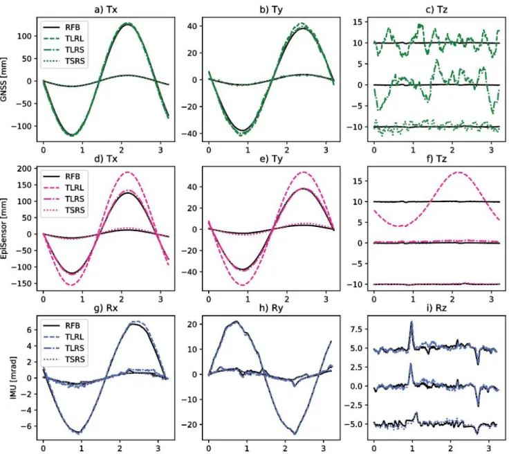
Figure 4: Zoom-in to a three second period at 300 s of the experiment. In black the robot feedback (RFB) and in colour the instruments.

(10)

Figure 5: Zoom-in to a three second period at 300 s of the experiment. In black the robot feedback (RFB) and in brown the KF state estimates displacement and velocity.

In Figure 4 and 5 each row of subfigures shows a three second zoom-in at 300 s of the simulated motion with the recorded RFB signal in black and additionally an instrument (a-i) or the KF estimated quantity (j-o) in color. All three experiments TLRL, TLRS and TSRS are shown per subfigure.

large rotations (TLRL) distort instrument records more small rotations (TLRS, TSRS) distort instrument records less High noise level of GNSS in z-component

KF estimates substantially better than instrument-only solution

short period ticks in z-component are reproduced by KF even though GNSS is the observation

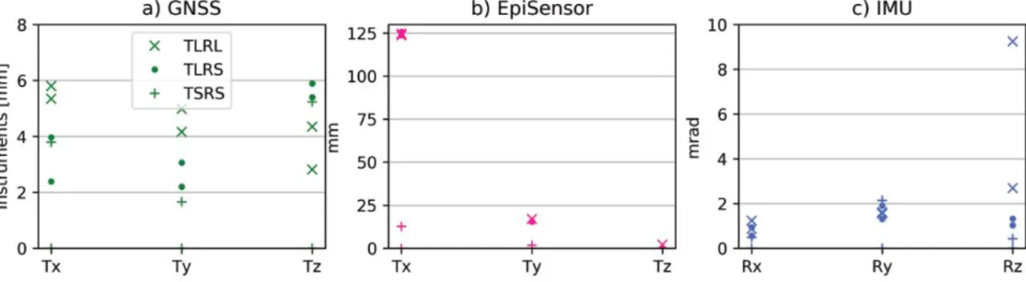
Analysis RMSE

for N = length of signal, a = Instrument or KF state estimate

RMSE = √∑

^N_n=0

^(a−RFB)_N ²ⁿ

(11)

Figure 6: Summary of KF performance in terms of RMSE. a-c show the three instruments in comparison to the robot feedback.

(12)

https://agu2020fallmeeting-agu.ipostersessions.com/Default.aspx?s=B7-F7-3C-23-70-CA-3E-13-83-40-08-0A-F6-4E-B0-C1&pdfprint=true&gue… 11/17

three experiments).

(13)

6. RESULTS II - FULL TIME SERIES OF KF FUSION

The robot feedback (RFB) of the TLRL experiment is now shown with the full KF state estimates in the Figure below. The figure additionally shows the RMSE of the difference between the two plotted time series. While there is still some residual motion that cannot be resolved by our filter, the overall fit is substantially better than taking each sensor individually.

long periods are tracked short periods are tracked

noise level is lower than in GNSS observations

(14)

For completeness the Experiment TSRS is shown below.

(15)

(16)

7. CONCLUSION

Benefits of our KF

Taking advantage of each instrument Better ground motion realization

The future of structural and seismic monitoring stations

Limitations of our KF

only for large motions

High quality GNSS positions necessary Good timing is essential

(17)

ABSTRACT

Shaking from earthquakes is a complex set of six components (6C) that make up the ground motion, containing both translations and rotations. Nonetheless, state-of-the-art earthquake monitoring stations only include accelerometers and GNSS to record the strong ground motion. The inertial accelerometer sensors directly measure the translational part of the motion, though rotations contaminate this output and are difficult to quantify. GNSS is less sensitive to rotations but can only resolve large amplitudes and long period ground motion. Therefore, the future design of monitoring stations should include a rotational sensor to allow a complete reconstruction of the ground motion.

We have built a monitoring station that combines an accelerometer and rotational sensor both sampling at 250 Hz, with a GNSS receiver and antenna determining coordinates with a lower sampling rate of 100 Hz. The three instruments have been fixed to a platform attached to the top of an industrial six-axis robot arm, while the arm performs simulated ground motions with high accuracy and repeatability. The robot records its own feedback loop including position and orientation of the platform, which serves as the ground truth of the performed trajectory. This allows us to compare all the results obtained to the actually performed trajectory of the robot.

We designed a 6C Kalman filter that combines the three instrument records using an optimal equation design and optimal tuning of the parameters. It includes time domain tilt correction of the acceleration and subsequent estimation and correction of the instrument records to get the state vector consisting of displacement and velocity. The developed framework and sensing scheme is able to output rotation-free, broadband and precise 3C translations as well as drift-free and precise 3C rotations.

(18)

REFERENCES

Farrell, W. A gyroscopic seismometer: Measurements during the borrego earthquake. Bulletin of the Seismological Society of America 1969, 59, 1239–1245.

Graizer, V.M. Inertial Seismometry Methods.Izv. USSR Acad. Sci., Phys. Solid Earth 1991, 27, 51–61.

Lin, C.J.; Huang, H.P.; Liu, C.C.; Chiu, H.C.Application of rotational sensors to correcting rotation-induced effects on accelerometers.Bulletin of the Seismological Society of America 2010, 100, 585–597. doi:10.1785/0120090123.

Assessing a 6C Kalman filter using experimental datasets from an industrial robot

Conference Poster

Assessing a 6C Kalman filter using experimental datasets from an industrial robot

Assessing a 6C Kalman Filter using

Experimental Datasets from an Industrial Robot

Yara Rossi, Konstantinos Tatsis, Mudathir Awadaljeed, Konstantin Arbogast, Eleni Chatzi, Markus Rothacher, John Clinton

1. MOTIVATION

2. EXPERIMENT SETUP

3. ROBOT REPEATABILITY

4. 6C KALMAN FILTER (KF)

State Equation

Observation Equation

0 3×3

0 3×3

0 3×3

0 3×3

0 3×3

5. RESULTS I - QUALITY

Analysis Timeseries

Analysis RMSE

RMSE = √∑

6. RESULTS II - FULL TIME SERIES OF KF FUSION

7. CONCLUSION

Benefits of our KF

Limitations of our KF

ABSTRACT

REFERENCES

0 _3×3

0 _3×3

0 _3×3

0 _3×3

0 _3×3