3-D Magnetotelluric Image of Offshore Magmatism at the
1
Walvis Ridge and Rift Basin
2
Marion Jegen1, Anna Avdeeva1,2, Christian Berndt1, Gesa Franz1, Björn Heincke1,3, 3
Sebastian Hölz1, Anne Neska4, Anna Marti5, Lars Planert1,6, J. Chen1,, Heidrun Kopp1, 4
Kiyoshi Baba7 , Oliver Ritter8, Ute Weckmann8, Naser Meqbel8 and Jan Behrmann1. 5
1Geomar, Helmholtz Centre for Ocean Research, Wischhofstr. 1-3, 24148 Kiel, Germany
6
2now at University of Leicester, University Road, Leicester LE1 7RH, United Kingdom
7
3now at GEUS, Øster Voldgade 1, 1350 Copenhagen, Denmark
8
4Institute of Geophysics, Polish Academy of Science, ul. Księcia Janusza 64, 01452 Warsaw, Poland
9
5University of Barcelona, C. Marti I Franques, 08028 Barcelona, Spain
10
6now at Forschungsanstalt für Wasserschall und Geophysik, WTD71, Klausdorfer Weg 2, D-24148
11
Kiel, Germany
12
7Earthquake Research Institute, The University of Tokyo, 1-1-1 Yayoi, Bunkyo-ku, Tokyo 113-0032,
13
Japan
14
8GFZ German Research Centre for Geosciences, Telegrafenberg 14473, Potsdam, Germany 15
1. Abstract 16
The Namibian continental margin marks the starting point of the Tristan da Cunha 17
hotspot trail, the Walvis Ridge. This section of the volcanic southwestern African 18
margin is therefore ideal to study the interaction of hotspot volcanism and rifting, 19
which occurred in the late Jurassic/early Cretaceous. Offshore magnetotelluric data 20
image electromagnetically the landfall of Walvis Ridge. Two large-scale high 21
resistivity anomalies in the 3-D resistivity model indicate old magmatic intrusions 22
related to hot-spot volcanism and rifting. The large-scale resistivity anomalies 23
correlate with seismically identified lower crustal high velocity anomalies attributed 24
to magmatic underplating along 2-D offshore seismic profiles. One of the high 25
resistivity anomalies (above 500 Ωm) has three arms of approximately 100 km width 26
and 300 km to 400 km length at 120 degree angles in the lower crust. One of the arms 27
stretches underneath Walvis Ridge. The shape is suggestive of crustal extension due 28
to local uplift. It might indicate the location where the hot-spot impinged on the crust 29
prior to rifting. A second, smaller anomaly of 50 km width underneath the continent 30
ocean boundary may be attributed to magma ascent during rifting. We attribute a low 31
resistivity anomaly east of the continent ocean boundary and south of Walvis Ridge to 32
the presence of a rift basin that formed prior to the rifting.
33
2. Introduction 34
Passive margins bordering the South Atlantic oceanic basin were active during the 35
Late Jurassic and Early Cretaceous when Western Gondwana ruptured and the South 36
Atlantic Ocean opened from south to north (Light et al., 1993; Macdonald et al., 37
2003). These margins offer a unique opportunity to study ancient geological processes 38
linking magmatism, continental extension, crustal breakup and subsidence during and 39
after rifting.
40
The South Atlantic passive margins can be grouped into three provinces based on 41
crustal structure and bathymetric expression: (1) The province south of Walvis Ridge, 42
offshore northern Namibia and south of the Florianopolis Basement High and Rio 43
Grande Rise offshore southern Brazil. Here, magmatism was voluminous, and formed 44
volcanic wedges broader than 100 km within the crust (Franke et al., 2007). These 45
wedges are manifested as seaward dipping reflectors (SDR) in seismic reflection 46
sections on the conjugate Namibian (Elliott et al., 2009; Gladczenko et al., 1998) and 47
Argentine margins (Franke et al., 2007). (2) The province adjacent to Walvis Ridge 48
and Rio Grande Rise. These parts of both margins are dominated by magmatism, with 49
its continental extensions into the Paraná Basalt Province and the Etendeka Plateau 50
attesting to possible activity of the Tristan da Cunha hot spot (O’Connor and Duncan, 51
1990). (3) The province north of Walvis Ridge and Rio Grande Rise, the margin of 52
eastern Brazil and the counterpart offshore Congo and Angola. These margins also 53
experienced volcanism during break up, but syn-rift and early post-rift evolution was 54
dominated by the formation of Aptian salt, shallow water carbonates, and clastic 55
sediments.
56 57
Shore line crossing geophysical and geological experiments have been carried out in 58
the Namibian central province at the landfall of Walvis Ridge within the framework 59
of the priority program SPP1375 SAMPLE: South Atlantic Margin Processes and 60
Links with onshore Evolution project. The ridge constitutes the bathymetric 61
expression of the interaction of the Tristan da Cunha hot spot with the opening of the 62
South Atlantic through a 1,500 km long bathymetric high of up to 2,000 m with a 63
strike direction of NE-SW. To the north, the ridge bathymetry sharply terminates 64
against the Florianopolis fracture zone (FFZ) (Sibuet et al., 1984). Seismically imaged 65
Moho shows that thickened oceanic crust underlies Walvis Ridge, whereas the 66
oceanic crust north of the fracture zone is much thinner (Fromm et al., 2015). It has 67
been suggested that the crust, which initially formed to the north of Walvis Ridge, has 68
been sheared through an eastward ridge jump in the initial opening phase along the 69
FFZ and transferred to the South American margin as the Sao Paolo Plateau (Sibuet et 70
al., 1984), but there is no conclusive geophysical evidence for this and this ridge jump 71
is not included in the newest plate reconstructions for the South Atlantic (Seton et al., 72
2012). Walvis Ridge itself is underlain by a lower crustal high velocity anomaly from 73
landfall over a length of approximately 300 km (Fromm et al., 2015), which may be 74
attributed to underplating related to the Tristan da Cunha hot spot. Onshore 75
underplating has been documented by high seismic vp/vs ratios (> 1.8) and thickened 76
oceanic crust at the northern end of the landfall (Heit et al., 2015) and as a zone of 77
increased vp velocity (> 7.5 km/s) of approximately 100 km width beneath the landfall 78
of Walvis Ridge (Ryberg et al., 2015). The Tristan da Cunha plume gave rise to only 79
a small hot-spot, i.e. plume surface expression on the seafloor, based on these seismic 80
studies.
81 82
However velocity models on land are sparse and offshore only 2-D seismic profiles 83
exist. In order to better assess the region of impact coherently over a regional scale, 84
we carried out a magnetotelluric (MT) experiment to derive a regional 3-D resistivity 85
model. Comparison of the large-scale resistivity image to regional seismic models 86
and a density model based on satellite data and seismic information (Maystrenko et 87
al., 2013) provides additional constraints on magmatism. Based on this resistivity 88
model we analyze the rifting sequence and magmatic evolution of Walvis Ridge on a 89
regional scale and further constrain the link between the Tristan da Cunha hotspot and 90
the opening of the South Atlantic.
91 92
3. Marine MT experiment 93
Electrical conduction in rocks is dominated by ionic conduction within pore fluids 94
(typically water or partial melt), leading to a first order dependence of bulk resistivity 95
on the amount of pore fluid within the rock matrix. A less common conducting 96
mechanism occurs along particular electrically conductive minerals such as graphite 97
or metal containing minerals (Palacky, 1987; Keller, 1987). Both conducting 98
mechanisms are dependent on temperature.
99
Dry rocks with low porosity such as old deep volcanic intrusions have increased 100
resistivity (Kariya and Shankland, 1983; Shankland and Ander, 1983; Palacky, 1987), 101
sediments with larger fluid filled pore fraction have a lower resistivity. Metamorphic 102
rocks have an even lower resistivity if they contain graphite or other electrically 103
conducting minerals. Shear zones are for example often associated with low electrical 104
resistivity due to the fact that they either act as pathways of fluids or contain graphite.
105
The MT method is an electromagnetic method that uses natural variations of the 106
Earth’s magnetic field as an electromagnetic source. It has first been proposed by 107
Cagniard (1953) and has been discussed in a variety of textbooks, most recently by 108
Chave and Jones (2013). The MT impedance is the Earth’s response to this natural 109
electromagnetic source and represents resistivity variations within the Earth. The 110
impedance is a complex valued matrix with four elements and is derived from 111
measurements of orthogonal electric and orthogonal magnetic field variations. The 112
elements of the impedance matrix are related to the ratio of horizontal electric and 113
magnetic field variations along the two coordinate axes at a particular period.
114
Impedance values at increasing periods contain information about resistivity 115
structures at increasing depth. As opposed to active source seismic data and similar to 116
potential field data, the MT data are not only sensitive to the region within the 117
measurement array, but also influenced by electrical resistivity variations beyond the 118
array of sites. The sensitivity to resistivity variations beyond the measurement array 119
decreases with increasing distance from the array and decreasing period. A resistivity 120
structure of the subsurface is derived in a final step from the data via inversion.
121
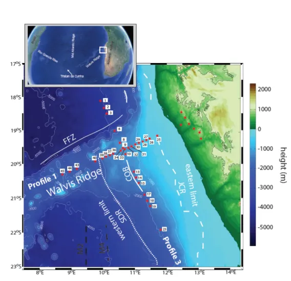
For the MT experiment in Namibia we acquired data offshore along two orthogonal 122
profiles, one parallel and one perpendicular to Walvis Ridge (Figure 1). Along these 123
profiles we occupied 45 sites in total with a spacing of approximately 10 km apart.
124
The profile orthogonal to Walvis Ridge ran along the ocean continent boundary, the 125
profile along Walvis Ridge placed in line with the land profiles along one of the few 126
roads in this region leading into the continent. The offshore data were acquired during 127
two deployments and recoveries on RV Maria S. Merian cruises MSM 17-1 and MSM 128
17-2 with ocean bottom electromagnetic (OBEM) instruments developed at 129
GEOMAR. The bottom time of the OBEM instruments was around 3 weeks, with 130
continuous recordings at a sampling rate of 1 Hz of two orthogonal horizontal electric 131
fields and three orthogonal magnetic fields (using a three component fluxgate 132
magnetometer) as well as tilt and temperature readings. The offshore data were 133
complemented with a subset of seven onshore stations with 5-component (two 134
orthogonal electric and 3 orthogonal magnetic) broadband MT instruments (10 kHz – 135
1 mHz) from a land MT grid run by GFZ Potsdam (Kapinos et al., 2016). These 136
coastal sites were essential for the derivation of the 3-D resistivity model since the 137
data contain information about the strong conductivity contrast at the Namibian coast.
138
The electromagnetic coast effect causes a particularly strong distortion at the coast. If 139
this boundary is not constrained by data on both sides or through a good priori 140
conductivity model on the opposing site of the array, it can lead to a strongly distorted 141
resistivity model (Worzewski et al., 2012).
142
From the acquired offshore data, only data from 32 out of 45 sites could be used for 143
further analysis. At 13 sites, either loss of data on some channels, lack of time 144
synchronization or electronic noise on the electric field channels prevented further 145
analysis.
146
The processing of the data to compute the impedance as a function of period consists 147
of several steps: First we corrected the electric and magnetic field variations for 148
instrument tilt and then we rotated the data to a single coordinate system (x, y, z 149
pointing northward, eastward and downwards, respectively). To calculate the 150
impedance from our time series, we used the bounded influence algorithm (Chave and 151
Thomson, 2004) and the multi-station scheme (Egbert, 1997). We obtained the 152
impedance tensors for frequencies ranging from 0.1 Hz to 10-4 Hz for the offshore 153
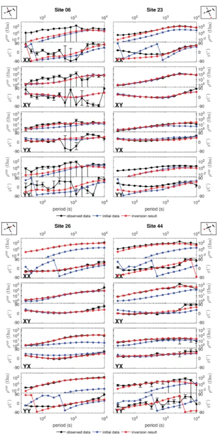
data. Examples of the complex valued impedance, expressed as apparent resistivity 154
and phase for all four elements of the impedance matrix as a function of period are 155
displayed in Figure 2. We show observed data for stations at which the data 156
demonstrate both high (sites 23, 26 and 4) and moderate quality data (site 6).
157
The magnetotelluric impedance matrix contains information about whether the 158
variations in the subsurface electrical resistivity sensed by the data are predominantly 159
1-D, 2-D or 3-D. Based on a dimensionality analysis described by Marti et al. (2009), 160
we observe that the data has a clear 3-D character at almost all sites. The 3-D 161
resistivity variations seen in the data can be attributed to the rough topography 162
(topographic high of Walvis Ridge running roughly orthogonal to the strong 163
resistivity contrast across the coast) and 3-D resistivity variations within the seafloor.
164
We therefore inverted the data to find a 3D resistivity model, taking into consideration 165
the complex seafloor bathymetry. although the experiment was originally set up for 166
two 2D profiles. Since MT data is sensitive to resistivity variations well beyond the 167
site location (especially for large period datasets as in this study), the error introduced 168
in the derived 3D model through the unequal site distribution across the survey area is 169
smaller than neglecting the complex and pronounced 3D bathymetry. The model 170
derived here is therefore more complete than the initial 2-D model presented by 171
Kapinos et al. (2016) based on an amphibious profile containing the offshore data 172
along profile 1.
173
A 3-D resistivity model of the Walvis Ridge area was obtained using a 3-D MT 174
inversion code (Avdeeva et al., 2012; Moorkamp et al., 2010). The code allows 175
positioning of MT sites at the seafloor and inclusion of bathymetry. The bathymetry 176
was approximated with a rectilinear mesh where horizontal cell sizes are constant 177
throughout the whole 3-D inversion volume. In addition, the modeling mesh is 178
embedded in a 1-D layered background. In our case, the volume of interest covers the 179
ocean in the west and continental crust to the east, such that a single 1-D background 180
model is inadequate. To overcome this problem, we extended the inversion mesh to 181
the sides so that the influence of a single 1D background model, inadequately 182
representing both the ocean- and land-side of the model simultaneously, is negligible.
183
There is a tradeoff between available computational resources and the accuracy of the 184
inverse problem solution. The mesh has to be fine enough to approximate the 185
bathymetry of the seafloor and to achieve accurate solutions for smaller period data, 186
yet not so large that computation time and memory requirements become unrealistic.
187
The mesh must also match the survey geometry and resolution of the MT method, i.e.
188
horizontal discretization should not be much smaller than the distance between 189
adjacent sites. Due to failure to recover data at some stations, the spacing is as large as 190
60 km in some regions. Taking all these considerations into account, we chose a mesh 191
consisting of 96×92×34 cells and covering an area of 960×920×300 km3. The 192
horizontal dimensions of the cells are 10 km, while the vertical cell sizes are 193
increasing with depth from 100 m to 50 km.
194
The starting model included the Atlantic Ocean (0.3 Ωm) and a crude bathymetry of 195
Walvis Ridge with a 1 Ωm sediment layer. If we do not include a sediment layer in 196
the starting model the inversion does not converge. Below the sediments the model 197
consists of a homogeneous half-space. We ran numerous inversions varying the 198
thicknesses of the sedimentary layer and resistivity of the initial half-space while 199
considering different data weights, error floors, and regularization strategies. Here, we 200
present our inversion result, which based on our testing, delivers the most credible 201
results. For this inversion run we started with a 3 km sediment layer with a 500 Ωm 202
half-space below. We used smooth regularization, with a regularization functional 203
based on a gradient operator, and adopt a cooling strategy for choosing the 204
regularization parameters. This means that during the first stages of the inversion we 205
require smooth resistivity models. This constraint is then gradually relaxed. We 206
furthermore assume a typical error floor of 5% in the impedance data. Due to the fact 207
that the starting model already contains the ocean, sediments, and a crude 208
approximation of the bathymetry, the modeled impedance due to this starting model, 209
termed initial data, fits the observed data with a relatively low RMS misfit of 5.6. The 210
inversion of this starting model to our final model produces modeled data, termed 211
predicted data, with an RMS misfit of 2.27. The misfit could not be reduced any 212
further, which we attribute to the relatively coarse bathymetry approximation with a 213
rectilinear mesh.
214
A comparison of initial and predicted data with the observed apparent resistivities and 215
phases is shown in Figure 2 for exemplary individual sites. The inversion significantly 216
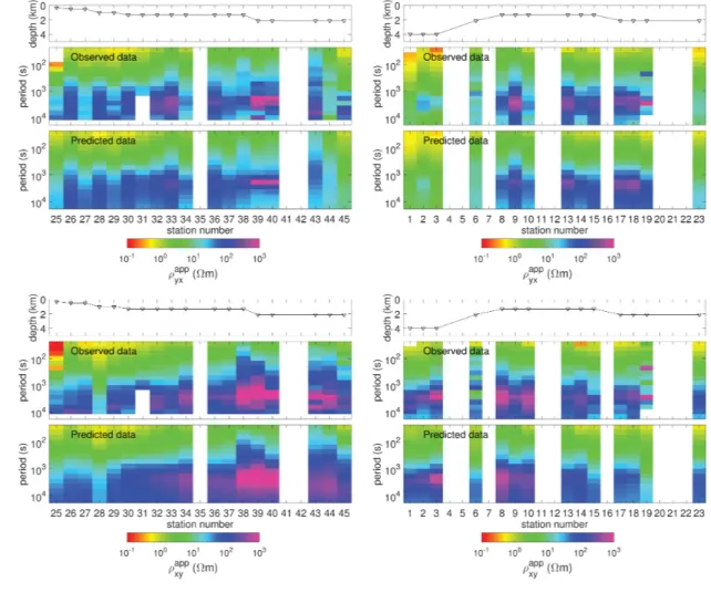
improves the data fit compared to the predicted data of the initial model. An overall 217
comparison of predicted and observed data for the off-diagonal elements of the 218
impedance is shown in Figure 3 in the form of pseudo sections of apparent resistivity 219
and phase as a function of period.
220
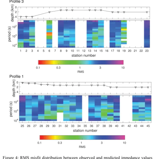
In order to validate the resistivity model obtained by the inversion, RMS values for 221
individual sites and periods are shown in Figure 4. For most sites and periods the 222
RMS value is below 3. The predicted data for sites 1, 2, 23, 25 and 45, all of which 223
are located at the end of the profiles, do not show a satisfactory fit to the observed 224
data. These sites, but for site 25, are located at the deepest parts of the profiles 225
offshore, where signal to noise ratio is smallest due to increased absorption of 226
electromagnetic energy by the overlying conductive ocean. Furthermore the vertical 227
grid size, which increases with depth, might be too large at these stations to model the 228
underlying subsurface resistivity variations in the upper part of the model or changes 229
of bathymetry occurring in the region. This would explain why the increased misfit is 230
particularly strong at smaller periods. Very good data fits observed for sites 6 and 19 231
should be attributed to the fact that the data quality at these sites was very poor (see 232
site 6 in Figure 2) and as a consequence data errors large.
233
4. Results 234
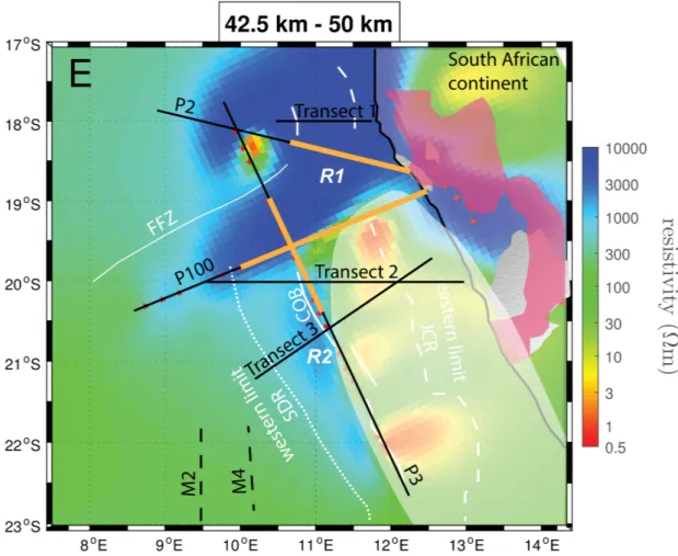
We present our resistivity model as five horizontal slices for depths of 8.5 km-10 km, 235
12.5 km -15km, 15 km - 20 km, 25 km - 30 km and 42.5 km - 50 km shown in Figure 236
5. On these horizontal slices, the coastline is superimposed as a black line. The 237
Etendeka flood basalt regions are shown as textured areas. Other main geological 238
features are shown as white lines and have been derived from seismic transects 1 to 4 239
in Gladczenko et al. (1998). The locations of these transects are marked by black lines.
240
The seismically inferred continent-ocean boundary (COB) is shown as a solid line and 241
is defined as the western termination of the lowermost seaward dipping reflector.
242
Gladczenko et al. (1998) inferred that a late Jurassic- early Cretaceous rift basin (JCR) 243
formed prior to the break up. The dashed line marks its eastern limit based on seismic 244
data.
245
Before we discuss the particular features of the resistivity model, we would like to 246
point out that the model is not equally well resolved everywhere. As discussed in the 247
previous section, MT data is generally sensitive to resistivities beyond the array, but 248
resolution decreases with increasing distance. We therefore consider small-scale 249
variations on the continent east of our land stations as not well resolved. A land data 250
set (see Kapinos et al., 2016 for station lay out) is currently being analysed through a 251
3-D inversion and will probably give a higher resolution image of this area. The land 252
data also contain short period data, which will allow the derivation of higher 253
resolution models in the upper crust.
254
The shallowest slice through our model is characterized by a number of smaller scale 255
anomalies. They mainly occur in the vicinity of sites where the predicted and 256
observed short period data exhibit a large misfit (Figure 4). Our relatively coarse 257
gridding of the model cannot reliably invert for these anomalies and we do not 258
consider them in the further discussion.
259
On the other hand, two large-scale resistivity anomalies north (high resistivity, 260
marked as R1 in Figure 5) and south (low resistivity, marked as C in Figure 5) of 261
Walvis Ridge are well resolved. The resistive anomaly R1 persists through all depth 262
slices, and extends further underneath Walvis Ridge and along a region south of 263
Walvis Ridge underneath the coast with increasing depth. It can therefore be regarded 264
as a large-scale, crustal/upper lithospheric mantle anomaly. At depths below 15 km, a 265
second region of high resistivity (R2 in Figure 5) underneath the COB south of 266
Walvis Ridge appears, which persists down to the base of our model.
267
The low resistivity feature also persists through all depth slices. However, the 268
sensitivity of MT data is reduced beneath conducting regions. Sensitivity studies have 269
shown that the model in this region is resolved well down to a depth of approximately 270
25 km. We have therefore blended out the low resistivity zone in the two lowermost 271
slices of our model.
272
For the discussion of the current inversion model we will concentrate on these main 273
large-scale features. In order to determine their tectonic origin, we will compare the 274
resistivity features to other geophysical data from the region, i.e. mainly offshore 275
seismic data. For the discussion of the resistive region on land, we will furthermore 276
compare the results to a density model, which has been derived by Maystrenko et al.
277
(2013) and which partly overlaps our study region. After verification of our model 278
with these data sets, we will interpret the observed spatial pattern in terms of their 279
tectonic-magmatic implication for the opening of the South Atlantic.
280
High resistivity zone R1 (Magmatic Intrusions Walvis Ridge and Coast):
281
MT data are generally not very sensitive to the precise resistivity value within a 282
resistive feature. While the data require a resistivity contrast to the surrounding model 283
in the area shaded in dark blue representative of resistivities above 1,000 Ωm (Figure 284
5), models where this region is changed to values of down to 500 Ωm fit the data 285
equally well.
286
The outline of the offshore high resistivity zone at depths of 25 km - 30 km and 42.5 287
km - 50 km correlates with a region of high seismic velocity anomalies in the lower 288
crust detected along co-occupied seismic refraction lines along the offshore MT 289
profiles (P3 and P100) as well as by a seismic line trending from the Angola basin 290
over the landfall of Walvis Ridge to the onshore domain (P2). The widths, where 291
increased lower crustal velocities have been detected along these profiles by Fromm 292
et al. (2015) are marked in orange in Figure 5 in our model slices at lower crustal 293
depth. The lower crustal high velocity region is interpreted as magmatic underplating 294
and has been attributed Fromm et al. (2015) as the region that has been affected by the 295
mantle plume. We therefore presume that the high resistive zone delineates the region, 296
where the ascending mantle plume from depth has imprinted the crust and lithospheric 297
mantle. Further evidence supporting our interpretation of the high resistivity zone on 298
land, where our model has arguably less resolution, comes from land studies. Heit et 299
al. (2015) report a strong increase in crustal thickness to 44 km and high seismic vp/vs
300
ratios of 1.89 on the African continent at the landfall of Walvis Ridge and northeast of 301
the landfall. Ryberg et al. (2015) detect increased lower crustal compressional 302
velocities above 7.5 km/s at the landfall of Walvis Ridge. Both authors attribute the 303
observations to magmatic underplating produced by the mantle plume during the 304
breakup of Gondwana. A gravity model (Maystrenko et al., 2013) of the South- 305
African margin overlaps up to about 17.5oS with our model, supplying spatial 306
information on the thickness of the continental crust within the longitudes of 9oE and 307
20oE for Walvis Ridge and the region south of Walvis Ridge. The study identifies a 308
lower crustal high-density body with densities of 2.95 kg/m3 (outlined in pink in 309
Figure 5 for our horizontal slices below 25 km), which coincides with the continental 310
part of our resistor.
311
At depths above 25 km some of the outer regions of the high resistivity anomaly R1 in 312
our model are replaced by decreasing resistivities indicative of higher porosity 313
perhaps due to more severe weathering of extrusive volcanic rocks (Planke and 314
Alvestad, 1999).
315
Based on the spatial coincidence of our resistivity anomaly and high lower crustal 316
velocities that were interpreted as magmatic underplating, we interpret the highly 317
resistive anomaly (R1 in Figure 5) as the region where magma has risen from the 318
mantle into the crust. We suggest that the anomaly delineates the extent of the Tristan 319
da Cunha plume impact.
320
Low resistivity zone C (Rift Basin):
321
While the boundary to the north of the resistivity anomaly R1 is diffuse, the southern 322
edge is characterized by an abrupt change towards low resistivities (anomaly C), just 323
south of our profile line along Walvis Ridge. Within the upper 10 km, the electrical 324
resistivity model exhibits a gradual change from a very low resistivity region in the 325
far east (< 3 Ωm) to intermediate resistivities of less than 10 Ωm to approximately 10 326
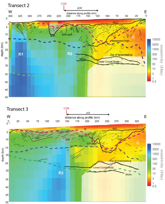
to 100 Ωm towards the COB. Comparison of the resistivity model with seismic results 327
along transect 2 and 3 (Figure 6) suggests that the likely cause of these low 328
resistivities is the presence of the rift basin that formed prior to the breakup of 329
Gondwana (Gladczenko et al., 1998). The region with resistivities of about 3 to 10 330
Ωm coincides with this Jurassic Cretaceous rift basin (JCR). Very low resistivities are 331
found in the area east of the boundary that separates the JCR from the old continental 332
belt. Within this region the seismic transects exhibit reflectors, which have been 333
interpreted as Late Precambrian shear zones (Clemson et al., 1997; Light et al., 1993), 334
or thrusts reactivated as Late Mesozoic extensional faults (Gladczenko et al., 1998).
335
Metamorphic minerals or potentially small amounts of graphite in the shear zone may 336
explain the extremely low resistivities (Haak and Hutton, 1986).
337
The lack of a rift basin north of Walvis Ridge may be due to an eastward relocation of 338
rifting and magmatism north of Walvis Ridge. This relocation may have sheared off 339
parts of the northern rift basin and its seaward dipping reflectors to the South- 340
American side along the Floreanopolis Fracture Zone (Sibuet et al., 1984; Elliot and 341
Berndt, 2009).
342 343
High resistivity zone R2 (Magmatism related to rifting along COB) 344
In the region below 10 km depth, west of the COB, we observe an increase of 345
resistivity in a band of approximately 100 km in which resistivities as high as several 346
100 Ωm (anomaly R2, Figure 6) are observed, which point to magmatic intrusions 347
related to the rifting and break up. The overlying extrusive basalt flows obscure deep 348
seismic reflections in this region and thus a seismic verification of the magmatic 349
intrusions, but for other volcanic rifted margins it has been shown that the seaward 350
dipping reflectors are frequently underlain by magmatic intrusions (Skogseid and 351
Eldholm, 1987). In terms of electrical resistivity, the overlying extrusive basalt flows 352
do not constitute a high resistivity anomaly, but exhibit resistivity in the range of tens 353
of Ωm to 100 Ωm. This value is typical for extrusive basalt layers in rifted margins 354
(Jegen et al., 2009).
355 356
East of the COB, seismic data indicate the presence of a high velocity lower crustal 357
body at a depth below 25 km. Our data show no indication of a high resistivity zone in 358
this region, which may be due to decreased sensitivity underneath the conductive 359
upper crust in this region. For further comparison, we have plotted the base of the 360
sediment within the JCR, the top of the high velocity body and the Moho as inferred 361
from gravimetric data (Maystrenko et al., 2013) in Figure 6. On the western, oceanic 362
part of the section the top of the lithospheric high resistivity region coincides with the 363
top of the lower crustal high velocity zone. East of the COB, the anomalous deep 364
crustal bodies derived from gravity and seismic data do not match, showing the 365
limitations of these crustal models.
366 367
5. Discussion: Implications for tectono-magmatic processes during the formation 368
of the Namibia volcanic rifted margin 369
The magnetotelluric data provide two additional constraints on the deep crustal 370
structure that were not known from seismic studies before. The highly resistive zone 371
underlying both the Walvis Ridge (also shown in the 2D model by Kapinos et al.
372
(2016) and the seaward dipping reflectors south of it (anomalies R1 and R2) coincide 373
with the bulk of the extrusive volcanic material encountered on the Namibian margin.
374 375
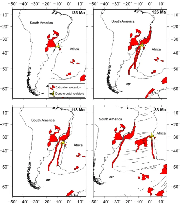
Near the coast the R1 anomaly consists of three arms protruding to the north along the 376
coastline, to the WSW along the Walvis Ridge, and to the SSE towards the Etendeka 377
flood basalt province (Figure 7). This 120 degree-spread between rift arms is typical 378
for point sources impinging into the crust, e.g. the rift arms of a shield volcano or the 379
ridge-ridge-ridge triple junction of the Afar hotspot, and we interpret the high 380
resistivity anomaly as the effect of the Tristan da Cunha hotspot where it impinged the 381
lithosphere at about 133 Ma (Müller et al., 1993) as shown in Figure 7a. Based on our 382
resistivity model, we would therefore place the Tristan da Cunha hotspot on the 383
African plate as suggested by Thompson and Gibson (1991) and Harry and Sawyer 384
(1992) and not on the South American plate as favored by O'Connor and Duncan, 385
(1990) and Turner et al. (1994).
386 387
After the short and vigorous continental flood basalt emplacement the plume 388
manifested itself in break-up volcanism with its center underneath the Walvis Ridge 389
but additional strong magma supply along the incipient break-up axis to the south 390
(Figure 7b). We interpret the resistive zone R2 that stretches south from the Walvis 391
Ridge underneath the center of the seaward dipping reflectors (along the COB) as the 392
magma conduits that fueled the volcanism leading to the emplacement of the seaward 393
dipping reflectors during the rifting stage and break-up stage. The resistivities here are 394
lower than those in the area of seismically imaged underplating farther north but 395
larger than those underneath the normal oceanic crust farther west. The sedimentary 396
basin and in particular the old rifted continental crust between the JCR and the coast 397
line show low resistivities that are considerably lower than normal continental crust.
398
6. Conclusion 399
In this study we present a 3-D resistivity model derived from a large-scale offshore 400
experiment that was augmented by seven coastal land stations. The resistivity model 401
reaching into the lithosphere maps the regions of increased magmatic production 402
through the Tristan da Cunha mantle plume and rifting, as comparison with other 403
available geophysical data in the area shows. The scale of the 3-D resistivity model 404
connects the piece-wise offshore information in form of 2-D seismic profiles with 405
onshore geology and provides valuable insight in the spatial distribution of increased 406
magmatic activity. The big high resistivity anomaly with three arms might represent 407
the rift arms that are expected to occur when the lithosphere is uplifted by a mantle 408
plume. The narrow resistive zone striking along the COB, west of the low resistivity 409
rift basin, is most likely related to magmatism during the break up of the continent.
410
The regional extent of the offshore 3-D experiment presented here and by Baba et al 411
(this issue) is one of the largest-scale academic offshore experiment of this type 412
performed up to now, next to a recent study in the Alboran Sea (Garcia et al., 2015).
413
While the current model shows some encouraging results and we are confident about 414
the larger scale features, the methodology and inversion algorithms may be further 415
improved in terms of resolution of the inversion model in the upper region. The large 416
orthogonal topography variations due to Walvis ridge and the coast make rectilinear 417
meshes not optimal as a large portion of the computationally feasible grid is used up 418
for representing the topography.
419
Acknowledgements 420
We thank the captain and the crew of R/V Maria S. Merian for the professional and 421
friendly support of the scientific work in the cruises. This work was supported by the 422
German Research Foundation (DFG) as part of the Priority Program SPP1375 and the 423
Future Ocean program of Kiel Marine Sciences. The computations were performed 424
using the ALICE High Performance Computing Facility at the University of Leicester.
425
7. References 426
Avdeeva, A., Avdeev, D., Jegen, M., 2012. Detecting a salt dome overhang with 427
magnetotellurics: 3D inversion methodology and synthetic model studies.
428
GEOPHYSICS 77, E251–E263. doi:10.1190/geo2011-‐0167.1 429
Cagniard L.,1953. Basic theory of the magnetotelluric method of geophysical 430
prospecting, Geophysics, 18, 605–635.
431
Chave, A.D. and Jones G. A., 2013. The Magnetotelluric Method, Theory and 432
Practice, Cambridge University Press, ISBN 9780521819275.
433
Chave, A.D., Thomson, D.J., 2004. Bounded influence magnetotelluric response 434
function estimation. Geophysical Journal International 157, 988–1006.
435
doi:10.1111/j.1365-‐246X.2004.02203.x 436
Clemson, J., Cartwright, J., BOOTH, J., 1997. Structural segmentation and the 437
influence of basement structure on the Namibian passive margin. Journal of 438
the Geological Society 154, 477–482. doi:10.1144/gsjgs.154.3.0477 439
Coffin, M.F., Eldholm, O., 1994. Large Igneous Provinces: crustal structure, 440
dimensions, and external consequences. Rev. Geophys. 32, 1–36.
441
Egbert, G.D., 1997. Robust multiple-‐station magnetotelluric data processing.
442
Geophysical Journal International 130, 475–496. doi:10.1111/j.1365-‐
443
246X.1997.tb05663.x 444
Elliott, G.M., Berndt, C., Parson, L.M., 2009. The SW African volcanic rifted margin 445
and the initiation of the Walvis Ridge, South Atlantic. Mar Geophys Res 30, 446
207–214. doi:10.1007/s11001-‐009-‐9077-‐x 447
Franke, D., Neben, S., Ladage, S., Schreckenberger, B., Hinz, K., 2007. Margin 448
segmentation and volcano-‐tectonic architecture along the volcanic margin off 449
Argentina/Uruguay, South Atlantic. Marine Geology 244, 46–67.
450
doi:10.1016/j.margeo.2007.06.009 451
Fromm, T., Planert, L., Jokat, W., Ryberg, T., Behrmann, J.H., Weber, M.H., 452
Haberland, C., 2015. South Atlantic opening: A plume-‐induced breakup?
453
Geology 43, 931–934. doi:10.1130/G36936.1 454
Garcia, X., Seillé, H., Elsenbeck, J., Evans, R.L., Jegen, M., Hölz, S., Ledo, J., Lovatini, 455
A., Martí, A., Marcuello, A., Queralt, P., Ungarelli, C., Ranero, C.R., 2015.
456
Structure of the mantle beneath the Alboran Basin from magnetotelluric 457
soundings. Geochem. Geophys. Geosyst. 16, 4261–4274.
458
doi:10.1002/2015GC006100 459
Gladczenko, T.P., Skogseid, J., Eldholm, O., 1998. Namibia volcanic margin. Mar 460
Geophys Res 20, 313–341.
461
Haak, V., Hutton, R., 1986. Electrical resistivity in continental lower crust.
462
Geological Society, London, Special Publications 24, 35–49.
463
doi:10.1144/GSL.SP.1986.024.01.05 464
Harry, D.L., Sawyer, D.S., 1992. Basaltic volcanism, mantle plumes, and the 465
mechanics of rifting: The Paraná flood basalt province of South America.
466
Geology 20, 207–210.
467
Heit, B., Yuan, X., Weber, M., Geissler, W., Jokat, W., Lushetile, B., Hoffmann, K.-‐H., 468
2015. Crustal thickness and V p/ V sratio in NW Namibia from receiver 469
functions: Evidence for magmatic underplating due to mantle plume-‐crust 470
interaction. Geophys. Res. Lett. 42, 3330–3337. doi:10.1002/2015GL063704 471
Jegen, M.D., Hobbs, R.W., Tarits, P., Chave, A., 2009. Joint inversion of marine 472
magnetotelluric and gravity data incorporating seismic 473
constraintsPreliminary results of sub-‐basalt imaging off the Faroe Shelf.
474
Earth and Planetary Science Letters 282, 47–55.
475
doi:10.1016/j.epsl.2009.02.018 476
Kapinos, G., Weckmann, U., Jegen-‐Kulcsar, M., Meqbel, N., Neska, A., Katjiuongua, 477
T.T., Hoelz, S., Ritter, O., 2016. Electrical resistivity image of the South 478
Atlantic continental margin derived from onshore and offshore 479
magnetotelluric data. Geophys. Res. Lett. 43, 154–160.
480
doi:10.1002/2015GL066811 481
Kariya, K.A. and Shankland, T. J., 1983. Electrical conductivity of dry lower crustal 482
rocks, Geophysics, 48, 52-‐61.
483
Keller, G.V., 1987. Rock and mineral properties, in Nabighian, M.N., ed., 484
Electromagnetic Methods in Applied Geophysics, Volume 1, Theory: Tulsa 485
Oklahoma, Society of Exploration Geophysicists, p. 13-‐51.
486
Light, M.P.R., Maslanyj, M.P., Greenwood, R.J., Banks, N.L., 1993. Seismic sequence 487
stratigraphy and tectonics offshore Namibia, in: Tectonics and Seismic 488
Sequence Stratigraphy. Geological Society, London, pp. 163–191.
489
Macdonald, D., Gomez-‐Perez, I., Franzese, J., Spalletti, L., Lawver, L., Gahagan, L., 490
Dalziel, I., Thomas, C., Trewin, N., Hole, M., Paton, D., 2003. Mesozoic break-‐
491
up of SW Gondwana: implications for regional hydrocarbon potential of the 492
southern South Atlantic. Marine and Petroleum Geology 20, 287–308.
493
doi:10.1016/S0264-‐8172(03)00045-‐X 494
Martí, A., Queralt, P., Ledo, J., 2009. WALDIM: A code for the dimensionality 495
analysis of magnetotelluric data using the rotational invariants of the 496
magnetotelluric tensor. Computers & Geosciences, 35, 2295–2303.
497
doi:10.1016/j.cageo.2009.03.004 498
Maystrenko, Y.P., Scheck-‐Wenderoth, M., Hartwig, A., Anka, Z., Watts, A.B., Hirsch, 499
K.K., Fishwick, S., 2013. Structural features of the Southwest African 500
continental margin according to results of lithosphere-‐scale 3D gravity and 501
thermal modelling. Tectonophysics 604, 104–121.
502
doi:10.1016/j.tecto.2013.04.014 503
Moorkamp, M., Heincke, B., Jegen, M., Roberts, A.W., Hobbs, R.W., 2010. A 504
framework for 3-‐D joint inversion of MT, gravity and seismic refraction data.
505
Geophysical Journal International 184, 477–493. doi:10.1111/j.1365-‐
506
246X.2010.04856.x 507
Müller, R.D., Royer, J.-‐Y., Lawver, L.A., 1993. Revised plate motions relative to the 508
hotspots from combined Atlantic and Indian Ocean hotspot tracks. Geology 509
21, 275–278.
510
O'Connor, J.M., Duncan, R.A., 1990. Evolution of the Walvis Ridge-‐Rio Grande Rise 511
Hot Spot System: Implications for African and South American Plate motions 512
over plumes. J. Geophys. Res. Solid Earth 95, 17475–17502.
513
doi:10.1029/JB095iB11p17475 514
Palacky, G.J., 1987. Resistivity characterization of geologic targets, in Nabighian, 515
M.N., ed., Electromagnetic Methods in Applied Geophysics, Volume 1, Theory:
516
Tulsa Oklahoma, Society of Exploration Geophysicists, 53-‐129.
517
Planke, S., Alvestad, E. 1999. Seismic volcanostratigraphy of the extrusive 518
breakup complexes in the northeast Atlantic: implications from ODP/DSDP 519
drilling, Proc. Ocean Drill. Program Sci. Results, 163, 1-‐16.
520
Ryberg, T., Haberland, C., Haberlau, T., Weber, M.H., Bauer, K., Behrmann, J.H., 521
Jokat, W., 2015. Crustal structure of northwest Namibia: Evidence for plume-‐
522
rift-‐continent interaction. Geology 43, 739–742. doi:10.1130/G36768.1 523
Seton, M., Müller, R.D., Zahirovic, S., Gaina, C., TORSVIK, T., Shephard, G., Talsma, 524
A., Gurnis, M., Turner, M., Maus, S., Chandler, M., 2012. Global continental and 525
ocean basin reconstructions since 200Ma. Earth-‐Science Reviews 113, 212–
526
270. doi:10.1016/j.earscirev.2012.03.002 527
Shankland, T.J. and Ander M.E., 1983. Electrical Conductivity, Temperature , and 528
Fluids in the Lower Crust. Journal of Geophysical Research, Vol. 88, B11, 529
9475-‐9484.
530
Sibuet, J.C., Hay, W.W., Prunier, A., Montadert, L., Hinz, K., Fritsch, J., 1984. The 531
Eastern Walvis Ridge and Adjacent Basins (South Atlantic): Morphology, 532
Stratigraphy, and Structural Evolution in Light of the Results of Legs 40 and 533
75, in: Initial Reports of the Deep Sea Drilling Project, 75, Initial Reports of 534
the Deep Sea Drilling Project. U.S. Government Printing Office.
535
doi:10.2973/dsdp.proc.75.108.1984 536
Skogseid, J., Eldholm, O., 1987. Early Cenozoic crust at the Norwegian continental 537
margin and conjugate Jan Mayen Ridge. J. Geophys. Res. 92, 11,471–11,491.
538
Thompson, R.N., Gibson, S.A., 1991. Subcontinental mantle plumes, hotspots and 539
pre-‐existing thinspots. Journal of the Geological Society 148, 973–977.
540
Turner, S., Regelous, M., Kelley, S., Hawkesworth, C., Mantowani, M., 1994.
541
Magmatism and continental break-‐up in the South Atlantic: high precision 542
40Ar-‐39Ar geochronology. Earth and Planetary Science Letters 121, 333–348.
543
Worzewski, T., Jegen, M., Swidinsky, A., 2012. Approximations for the 2-‐D coast 544
effect on marine magnetotelluric data. Geophysical Journal International, 189, 545
357–368. doi:10.1111/j.1365-‐246X.2012.05385.x 546
547
548
549
Figures 550
551
552
553
Figure 1: Experiment layout for the marine MT experiment. Inset shows the location of the 554
experiment and labeled major geological features relevant to the paperTwo profiles (profile 1 555
and profile 3) were occupied by OBEM stations. Red stars and numbers mark stations that 556
delivered data of sufficient quality to be included in the inversion. Overlain are labelled 557
geological features from Gladzenko et al. (1998) in white: The Floreanopolis Fracture Zone 558
(FFZ) (Sibuet et al., 1984), the continent-ocean boundary COB, the western end of SDR 559
sequences (dotted line) and the eastern border of the Jurassic-Creataceous Rift Basin (JCR, 560
dashed line). The eastern bound of the SDR sequence and western bound of the JCR coincide 561
with the COB.
562
563
Figure 2: Apparent resistivities and phases for few exemplary measurement sites. The chosen 564
sites represent data with moderate quality (left panel) and good quality (right panels) for all 565
four elements of the impedance tensor. Black curve show the observed data. Modeled data 566
based on the starting model (initial data) are depicted as blue lines. Red lines show the 567
predicted data of the final inversion model presented here.
568
569
Figure 3: Comparison of predicted and measured off-diagonal elements of the 570
impedance tensor given as apparent resistivity and phase for sites along Profile 100 571
(along Walvis Ridge) on the left and Profile 3 (across Walvis Ridge) on the right.
572 573 574
575
Figure 4: RMS misfit distribution between observed and predicted impedance values for 576
profile 3 (upper panel) and profile 1 (lower panel). The RMS was calculated at each site 577
and frequency based on the sum of the individual RMS for each impedance matrix 578
element. For the calculation we assumed a constant error given by the maximum error of 579
the impedance elements at this site and period.
580 581
582
583
584
585
586
Figure 5: Areal depth slices through the resistivity model representing the derived resistivity 587
at 8.5km-10km (A), 12.5km-15km (B), 15km-20km (C), 25km-30km (D) and 42km-50km 588
(E). Overlain are labelled geological features from Gladzenko et al. (1998) in white: The 589
Floreanopolis Fracture zone (FFZ), the continent-ocean boundary COB and the western end 590
of SDR sequences (dotted line) and the eastern border of the late Jurassic-early Cretaceous 591
Rift Basin (JCR, dashed line). The eastern bound of the SDR sequence and western bound of 592
the JCR coincide with the COB. Seismic profiles from Gladzenko (transect 1 to 4) and 593
Fromm et al., 2015 (P2, P3, P100) are shown as black lines. Orange line denote the 594
underplating inferred by Fromm et al, 2015 (panels D and E). Grey textured areas show 595
region of flood basalt. Positions of MT stations used in analysis are marked by red stars. Pink 596
area shows the outline of the continental high density lower crustal body as derived by 597
Maystrenko et al., 2013 (panels D and E). Please note that the high density body is cut off in 598
the north where their study area ends. Offshore lower crustal high density bodies have been 599
omitted due to clarity of figure.
600 601 602
603
Figure 6: Comparison of resistivity model with seismic data along transect 2 (upper panel) 604
and transect 3 (middle panel). The seismic data is represented as line drawing and taken from 605
a depth section in Gladzenko et al. (1998) together with his notation of the major geological 606
features: RUC denotes the Late Jurassic – Early Cretaceous rift basin, ORT the old rift 607
unconformity, TB top basalt and SDR seaward dipping reflector. The dashed magenta, blue 608
and green line denote the base of the sediments and top of lower crustal high velocity body 609
and the Moho as derived in a gravity data study by Maystrenko et al. (2013).
610 611
612
Figure 7: Plate tectonic reconstruction (Seton et al., 2012) showing the location of the high 613
resistivity anomaly through time placing the hotspot impingement underneath the African 614
Plate at 133 Ma and subsequent development of another high resistivity anomaly during the 615
emplacement of the seaward dipping reflectors between 133 Ma and 126 Ma. Outlines of 616
large igneous provinces based on Coffin and Eldholm (1994).
617