Calculating linear-response functions for finite temperatures on the basis of the alloy analogy model

Calculating linear-response functions for finite temperatures on the basis of the alloy analogy model

H. Ebert, S. Mankovsky, K. Chadova, S. Polesya, J. Min´ar, and D. K¨odderitzsch

Department Chemie/Phys. Chemie, Ludwig-Maximilians-Universit¨at M¨unchen, Butenandtstrasse 5-13, D-81377 M¨unchen, Germany (Received 4 December 2014; revised manuscript received 3 April 2015; published 27 April 2015)

A scheme is presented that is based on the alloy analogy model and allows one to account for thermal lattice vibrations as well as spin fluctuations when calculating response quantities in solids. Various models to deal with spin fluctuations are discussed concerning their impact on the resulting temperature-dependent magnetic moment, longitudinal conductivity, and Gilbert damping parameter. It is demonstrated that, by using the Monte Carlo (MC) spin configuration as input, the alloy analogy model is capable of reproducing the results of MC simulations on the average magnetic moment within all spin fluctuation models under discussion. On the other hand, the response quantities are much more sensitive to the spin fluctuation model. Separate calculations accounting for the thermal effect due to either lattice vibrations or spin fluctuations show that they give comparable contributions to the electrical conductivity and Gilbert damping. However, comparison to results accounting for both thermal effects demonstrates violation of Matthiessen’s rule, showing the nonadditive effect of lattice vibrations and spin fluctuations. The results obtained for bcc Fe and fcc Ni are compared with the experimental data, showing rather good agreement for the temperature-dependent electrical conductivity and the Gilbert damping parameter.

DOI:10.1103/PhysRevB.91.165132 PACS number(s): 72.10.Di,72.15.Eb,71.20.Be,75.10.−b

I. INTRODUCTION

Finite temperature often has a very crucial influence on the response properties of a solid. A prominent example for this is the electrical resistivity of perfect nonmagnetic metals and ordered compounds that take only a nonzero value with a characteristic temperature (T) dependence due to thermal lattice vibrations. While the Holstein transport equation [1,2] provides a sound basis for corresponding calculations, numerical work in this field has been done so far either on a model level or for simplified situations [3–6]. In practice the Boltzmann formalism is often adopted, using the constant-relaxation-time (τ) approximation. This is a very popular approach in particular when dealing with the Seebeck effect, as in this caseτ drops out [7,8]. The constant- relaxation-time approximation has also been used extensively when dealing with the Gilbert damping parameterα[9–11].

Within the description of Kambersky [10,12], the conductivity- and resistivitylike intra- and interband contributions to α show a different dependency on τ, leading typically to a minimum for α(τ) or equivalently for α(T) [10,11,13]. A scheme to deal with the temperature-dependent resistivity that is formally much more satisfying than the constant-relaxation- time approximation is achieved by combining the Boltzmann formalism with a detailed calculation of the phonon properties.

As was shown by various authors [14–17], this parameter-free approach leads for nonmagnetic metals in general to a very good agreement with experimental data.

As an alternative to this approach, thermal lattice vibrations have also been accounted for within various studies by quasistatic lattice displacements leading to thermally induced structural disorder in the system. This point of view provides the basis for the use of the alloy analogy, i.e., for the use of techniques to deal with substitutional chemical disorder, also when dealing with temperature-dependent quasistatic random lattice displacements. Examples of this are investigations on the temperature dependence of the resistivity and the Gilbert parameterαbased on the scattering matrix approach applied to layered systems [18]. The necessary average over many

configurations of lattice displacements was taken by means of the supercell technique. In contrast to this the configurational average was determined using the coherent potential approxi- mation (CPA) within investigations using a Kubo-Greenwood- like linear expression forα[19]. The same approach to deal with the lattice displacements was also used recently within calculations of angle-resolved photoemission spectra on the basis of the one-step model of photoemission [20].

Another important contribution to the resistivity in the case of magnetically ordered solids is given by thermally induced spin fluctuations [21]. Again, the alloy analogy has been exploited extensively in the past when dealing with the impact of spin fluctuations on various response quantities.

The representation of a frozen spin configuration by means of supercell calculations has been applied for calculations of the Gilbert parameter forα[18] as well as for the resistivity or conductivity [18,22,23]. Also, the CPA has been used for calculations of α [24] as well as the resistivity [21,25]. A crucial point in this context is obviously the modeling of the temperature-dependent spin configurations. Concerning this, rather simple models have been used [24], but also quite sophisticated schemes. Here one should mention the transfer of data from Monte Carlo simulations based on exchange parameters calculated in anab initioway [26] as well as work based on the disordered local moment (DLM) method [25,27].

Although the standard DLM does not account for transversal spin components it nevertheless allows representation of the paramagnetic regime with no net magnetization in a rigorous way. Also, for the magnetically ordered regime below the Curie temperature it can be demonstrated that the uncompensated DLM still leads for many situations to good agreement with experimental data on the so-called spin disorder contribution to the resistivity [21,25].

In the following we present technical details and ex- tensions of the so-called alloy analogy scheme which has already been used when dealing with the tempera- ture dependence of response quantities on the basis of Kubo’s response formalism [19,24]. Various applications will be presented for the conductivity and Gilbert damping

parameter accounting simultaneously for various types of disorder.

II. THEORETICAL FRAMEWORK

A. Configurational average for linear-response functions Many important quantities in spintronics can be formulated by making use of the linear-response formalism. Important examples for this are the electrical conductivity [28,29], the spin conductivity [30], and the Gilbert damping parameter [19,31]. Restricting attention here for the sake of brevity to the symmetric part of the corresponding response tensorχμνthis can be expressed by a correlation function of the form

χμν ∝ TrAˆμImG⁺AˆνImG⁺c. (1) It should be stressed that this is not a real restriction as the scheme described below has been used successfully when dealing with the impact of finite temperatures on the anomalous Hall conductivity of Ni [32]. In this case the more complex Kubo-Stˇreda or Kubo-Bastin formulation for the full response tensor has to be used [33].

The vector operator ˆA_μ in Eq. (1) stands, for example, in the case of the electrical conductivityσμν for the current density operator ˆjμ [29], while in the case of the Gilbert damping parameter αμν it stands for the torque operator ˆTμ

[9,19]. Within the Kubo-Greenwood-like equation (1) the electronic structure of the investigated system is represented in terms of its retarded Green function G⁺(r,r,E). Within multiple-scattering theory or the Korringa-Kohn-Rostoker (KKR) formalism,G⁺(r,r,E) can be written as [34–36]

G⁺(r,r,E)=

Z^m(r,E)τ^mn(E)Z^n×(r,E)

−δ_mn

Zⁿ(r,E)J^n×(r,E) (r_n−r_n) +Jⁿ(r,E)Z^n×(r,E) (rn−r_n). (2) Herer,rrefer to points within atomic volumes around sites Rm,Rn, respectively, with Zⁿ(r,E)=Z(rn,E)=Z(r− Rn,E) being a function centered at siteRn. Adopting a fully relativistic formulation [35,36] for Eq. (2), one gets in a natural way access to all spin-orbit-induced properties such as, for example, the anomalous and spin Hall conductivity [30,33,37] or the Gilbert damping parameter [19]. In this case, the functions Zⁿ andJⁿ stand for the regular and irregular solutions, respectively, to the single-site Dirac equation for site nwith the associated single-site scatteringtmatrixtⁿ . The corresponding scattering path operatorτⁿⁿ accounts for all scattering events connecting the sitesnandn. Using a suitable spinor representation for the basis functions the combined quantum number=(κ,μ) stands for the relativistic spin- orbit and magnetic quantum numbers κ andμ, respectively [35,36,38].

As has been demonstrated by various authors [28,29,39]

representing the electronic structure in terms of the Green function G⁺(r,r,E) allows chemical disorder in a random alloy to be accounted for by making use of a suitable alloy theory. In this case· · · cstands for the configurational average for a substitutional alloy with reference to the site occupation.

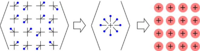
FIG. 1. (Color online) Configurational averaging for thermal lat- tice displacements: The continuous distributionP(Rn(T))for the atomic displacement vectors is replaced by a discrete set of vectors Rv(T) occurring with the probability xv. The configurational average for this discrete set of displacements is made using the CPA, leading to a periodic effective medium.

Corresponding expressions for the conductivity tensor have been worked out by Velick´y [28] and Butler [29] using the single-site coherent potential approximation which include in particular the so-called vertex corrections.

The CPA can be used to deal with chemical but also with any other type of disorder. In fact, by making use of the different time scales connected with the electronic propagation and spin fluctuations, the alloy analogy is exploited when dealing with finite-temperature magnetism on the basis of the disordered local moment model [27,40]. Obviously, the same approach can be used when dealing with response tensors at finite temperatures. In connection with the conductivity this is often called the adiabatic approximation [41]. Following this philosophy, the CPA has been used recently also when calculating response tensors using Eq. (1) with disorder in the system caused by thermal lattice vibrations [19,32] as well as by spin fluctuations [21,42].

B. Treatment of thermal lattice displacement

A way to account for the impact of the thermal displacement of atoms from their equilibrium positions, i.e., for thermal lattice vibrations, on the electronic structure is to set up a representative displacement configuration for the atoms within an enlarged unit cell (the supercell technique). In this case one has either to use a very large supercell or to take the average over a set of supercells. Alternatively, one may make use of the alloy analogy for the averaging problem. This allows in particular attention to be restricted to the standard unit cell.

Neglecting the correlation between the thermal displacements of neighboring atoms from their equilibrium positions the properties of the thermally averaged system can be deduced by making use of the single-site CPA. This basic idea is illustrated by Fig.1. To make use of this scheme a discrete set ofNv displacement vectorsR^qv(T) with probabilityx^qv

(v=1, . . . ,Nv) is constructed for each basis atomq within the standard unit cell that conforms with the local symmetry and the temperature-dependent root mean square displacement (u²T)^1/2according to

N_v

v=1

x_v^qR^q_v(T)²= u²_q

T. (3)

In the general case, the mean square displacement along the directionμ(μ=x,y,z) of the atomican either be taken from experimental data or represented by the expression based on

the phonon calculations [43]:

u²_i,μ

T = 3 2Mi

_∞

0

dωgi,μ(ω)1

ωcoth ω

2k_BT, (4) where h=2πis the Planck constant,k_B is the Boltzmann constant, andg_i,μ(ω) is a partial phonon density of states [43].

On the other hand, a rather good estimate for the root mean square displacement can be obtained using Debye’s theory. In this case, for systems with one atom per unit cell, Eq. (4) can be reduced to the expression

u²T = 1 4

3h² π²Mk_B D

( D/T)

D/T +1 4

(5) with ( D/T) the Debye function and D the Debye temperature [44]. Ignoring the zero-temperature term 1/4 and assuming a frozen potential for the atoms, the situation can be dealt with in full analogy to the treatment of disordered alloys on the basis of the CPA. The probability xv for a specific displacementvmay normally be chosen as 1/Nv. The Debye temperature _D used in Eq. (5) can be either taken from experimental data or calculated by representing it in terms of the elastic constants [45]. In general the latter approach should give more reliable results in the case of multicomponent systems.

To simplify notation we restrict or attention in the following to systems with one atom per unit cell. The indexqnumbering sites in the unit cell can therefore be dropped, while the index nnumbers the lattice sites.

Assuming a rigid displacement of the atomic potential in the spirit of the rigid muffin-tin approximation [46,47] the corresponding single-sitetmatrixt^loc=tⁿwith respect to the local frame of reference connected with the displaced atomic position is unchanged. With respect to the global frame of reference connected with the equilibrium atomic positions Rn, however, the corresponding t matrix t is given by the transformation

t =U(R)t^locU(R)⁻¹. (6) The so-called U transformation matrix U(s) is given in its nonrelativistic form by [46,47]

ULL(s)=4π

L

i^l+l−lCLLLjl(|s|k)YL(ˆs). (7) HereL=(l,m) represents the nonrelativistic angular momen- tum quantum numbers, j_l(x) is a spherical Bessel function, YL(ˆr) is the real spherical harmonics,CLLLis a corresponding Gaunt number, andk=√

Eis the electronic wave vector. We here use atomic Rydberg units for the energy E, which is measured with respect to the so-called muffin-tin zero. The relativistic version of theUmatrix is obtained by a standard Clebsch-Gordan transformation [38].

The various displacement vectorsRv(T) can be used to determine the properties of a pseudocomponent of a pseu- doalloy. Each of theNvpseudocomponents with|Rv(T)| = u^21/2T is characterized by a correspondingUmatrixU_v and atmatrix t_v. As for a substitutional alloy, the site diagonal configurational average can be determined by solving the multicomponent CPA equations within the global frame of

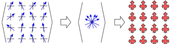
FIG. 2. (Color online) Configurational averaging for thermal spin fluctuations: The continuous distribution P( ˆen) for the ori- entation of the magnetic moments is replaced by a discrete set of orientation vectors ˆef occurring with a probability xf. The configurational average for this discrete set of orientations is made using the CPA, leading to a periodic effective medium.

reference:

τ_CPA=

N_v

v=1

xvτ_v, (8) τ_v =[(t_v)⁻¹−(t_CPA)⁻¹+(τ_CPA)⁻¹]⁻¹, (9) τ_CPA = 1

_BZ

_BZ

d³k[(t_CPA)⁻¹−G(k,E)]⁻¹, (10) where the underline indicates matrices with respect to the combined index . As was pointed out in previous work [42], the cutoff for the angular momentum expansion in these calculations should be taken as ll_max+1 with the l_max value used in the calculations for the nondistorted lattice.

In all calculations we have usedNv =14: increasing the set of directions for the atomic displacements led to only minor changes of the final results.

The first of these CPA equations represents the require- ment for the mean-field CPA medium that embedding of a component v should lead on the average to no additional scattering. Equation (9) gives the scattering path operator for the embedding of the component v into the CPA medium, while Eq. (10) gives the CPA scattering path operator in terms of a Brillouin zone integral withG(k,E), the so-called KKR structure constants.

Having solved the CPA equations, the linear-response quantity of interest may be calculated using Eq. (1) as for an ordinary substitutional alloy [28,29]. This implies that one also has to deal with the so-called vertex corrections [28,29]

that take into account that one has to deal with a configuration average of the typeAˆμImG⁺AˆνImG⁺c which in general will differ from the simpler productAˆ_μImG⁺cAˆ_νImG⁺c.

C. Treatment of thermal spin fluctuations

As for the disorder connected with thermal displacements, the impact of disorder due to thermal spin fluctuations may be accounted for by use of the supercell technique. Alternatively one may again use the alloy analogy and determine the necessary configurational average by means of the CPA as indicated in Fig.2. As for the thermal displacements in a first step a set of representative orientation vectors ˆef (withf = 1, . . . ,Nf) for the local magnetic moment is introduced (see below). Using the rigid spin approximation the spin-dependent partB_XCof the exchange-correlation potential does not change for the local frame of reference fixed to the magnetic moment

when the moment is oriented along an orientation vector ˆef. This implies that the single-sitetmatrixt^loc_f in the local frame is the same for all orientation vectors. With respect to the common global frame that is used to deal with the multiple scattering [see Eq. (10)] the tmatrix for a given orientation vector is determined by:

t =R( ˆe)t^locR( ˆe)⁻¹. (11) Here the transformation from the local to the global frame of reference is expressed by the rotation matricesR( ˆe) which are determined by the vectors ˆeor corresponding Euler angles [38]. Again the configurational average for the pseudoalloy can be obtained by setting up and solving the CPA equations in analogy to Eqs. (8)–(10).

D. Models of spin disorder

The central problem with the scheme described above is obviously the construction of a realistic and representative set of orientation vectors ˆef and probabilities xf for each temperatureT to be used in the subsequent calculation of the response quantity using the alloy analogy model. A rather appealing approach is to calculate the exchange-coupling parameters Jij of a system in an ab initio way [26,48,49]

and to use them in subsequent Monte Carlo (MC) simulations.

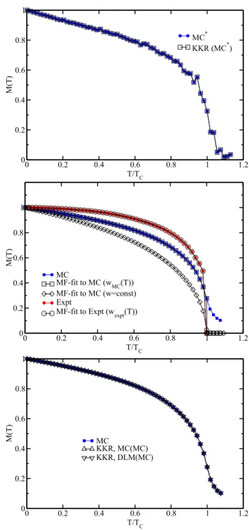
Figure 3 (top) shows results for the temperature-dependent average reduced magnetic moment of corresponding simula- tions for bcc Fe obtained for a periodic cell with 4096 atom sites. Note that these results have been obtained using the exchange coupling parameters calculated for the DLM state, modeling the disordered magnetic state above T_C that gave the best agreement with the experimental Curie temperature [27]. The MC calculations for Fe using a classical Heisenberg Hamiltonian have been discussed in [50] in more detail. In the case of Ni the calculations ofJij have been performed for the ferromagnetic (FM) state. The Curie temperature obtained via MC simulations is strongly underestimated, which was also discussed previously by many authors (see, e.g., [51]). The full line gives the value for the reduced magnetic moment of the MC cellM_MC∗(T)= mzT/m₀projected on thezaxis, calcu- lated for the last single Monte Carlo step (ˆzis the orientation of the total moment, i.e.,mTz; the saturated magnetic momentˆ at T =0 K is m₀= |mT=0|). This scheme is called MC^∗ in the following. In spite of the rather large number of sites (4096) the curve is rather noisy in particular when approaching the Curie temperature. Nevertheless, the spin configuration of the last MC step was used as an input for subsequent spin-polarized relativistic (SPR) KKR-CPA calculations using the orientation vectors ˆefwith the probabilityxf =1/Nfwith Nf =4096. As Fig.3(top) shows, the temperature-dependent reduced magnetic moment M_KKR(MC∗)(T) deduced from the electronic structure calculations follows one-to-one the Monte Carlo data M_MC∗(T). This is a very encouraging result for further applications (see below) as it demonstrates that the CPA although being a mean-field method and used here in its single-site formulation is nevertheless capable of reproducing results of MC simulations that go well beyond the mean-field level.

However, using the set of vectors ˆe_f of the scheme MC*

also for calculations of the Gilbert damping parametersαas a

0 0.2 0.4 0.6 0.8 1 1.2

T/T_C 0

0.2 0.4 0.6 0.8 1

M(T)

MC^* KKR (MC^*)

0 0.2 0.4 0.6 0.8 1 1.2

T/T_C 0

0.2 0.4 0.6 0.8 1

M(T) MC

KKR, MC(MC) KKR, DLM(MC)

0 0.2 0.4 0.6 0.8 1 1.2

T/T_C 0

0.2 0.4 0.6 0.8 1

M(T)

MCMF-fit to MC (w_MC(T)) MF-fit to MC (w=const) ExptMF-fit to Expt (w_expt(T))

FIG. 3. (Color online) Averaged reduced magnetic moment M(T)= mzT/|mT=0| along the z axis as a function of the temperatureT. Top: Results of Monte Carlo simulations using the scheme MC* (full squares) compared with results of subsequent KKR calculations (open squares). Middle: Results of Monte Carlo simulations using the scheme MC (full squares) compared with results using a mean-field fit with a constant Weiss field parameter wMC(TC) (open diamonds) and a temperature-dependent Weiss field parameterw_MC(T) (open squares). In addition experimental data (full circles) together with a corresponding mean-field fit obtained for a temperature-dependent Weiss field parameter wexpt(T). Bottom:

Results of Monte Carlo simulations using the scheme MC (full squares) compared with results of subsequent KKR calculations using the MC scheme (up triangles) and a corresponding DLM (down triangles) spin configuration, respectively.

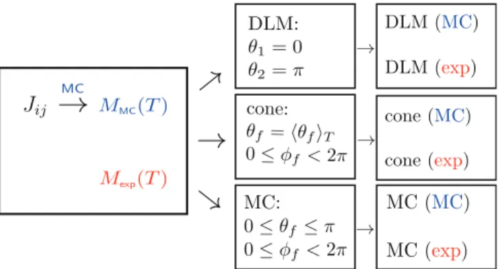
FIG. 4. (Color online) Overview of the different models used to treat spin disorder together with the notation used in the text. The starting point is a temperature-dependent magnetizationM(T) either (i) taken from experiment or (ii) obtained from a Monte Carlo sim- ulation that uses exchange-coupling constants from a first-principles electronic structure calculation. Three different models abbreviated as MC, DLM, and cone are then used to obtain a representative distribution of moments [weights and directions{x_f,eˆ_f(θ,φ)}] that in turn reproduceM(T). On the right in parentheses the source is given (“MC” or “expt” data) upon which the calculation of response quantities is based.

function of temperature led to extremely noisy and unreliable curves forα(T). For that reason an average has been taken over many MC steps (scheme MC) leading to a much smoother curve forM_MC(T) as can be seen from Fig.3 (middle) with a Curie temperatureT_C^MC =1082 K. As this enlarged set of vectors ˆef got too large to be used directly in subsequent SPR-KKR-CPA calculations, a scheme was worked out to get a set of vectors ˆefand probabilitiesxfthat is not too large but nevertheless leads to smooth curves forM(T).

The first attempt was to use the Curie temperature T_C^MC to deduce a corresponding temperature-independent Weiss field parameterw(TC) on the basis of the standard mean-field relation

w(TC)=3k_BT_C

m²₀ . (12)

This leads to a reduced magnetic moment curveM_MF(T) that shows by construction the same Curie temperature as the MC simulations. For temperatures betweenT =0 K andT_C, however, the mean-field reduced magnetic momentM_MF(T) is well below the MC curve [see Fig.3(middle)].

As an alternative to this simple approach we introduced a temperature-dependent Weiss field parameter w(T). This allows us to describe the temperature-dependent magnetic properties using the results obtained beyond the mean-field approximation. At the same time the calculation of the statistical average can be performed by treating the model Hamiltonian in terms of the mean-field theory. For this reason the reduced magnetic momentM(T), being a solution of the equation (see, e.g., [52])

M(T)=L wm²₀M(T) k_BT

, (13)

was fitted to that obtained from MC simulationsM_MC(T) with the Weiss field parameterw(T) as a fitting parameter, such that

w→limw(T)M(T)=M_MC(T), (14) withL(x) the Langevin function.

The corresponding temperature-dependent probabilityx( ˆe) for an atomic magnetic moment to be oriented along ˆe is proportional to exp(w(T)ˆz·e/kˆ _BT) (see, e.g., [52]). To calculate this value we usedNθandNφpoints for a regular grid for the spherical anglesθ andφcorresponding to the vector ˆ

ef:

x_f = sin(θf) exp[w(T)ˆz·eˆf/k_BT]

fsin(θf) exp[w(T)ˆz·eˆf/k_BT]. (15) Figure 5 shows the θ-dependent behavior of x( ˆe) for three different temperatures. As one notes, the mean-field (MF) fit to the MC results perfectly reproduces these data for all temperatures. This applies of course not only for the angular-resolved distribution of the magnetic moments shown in Fig.5but also for the average reduced magnetic moment recalculated using Eq. (13), shown in Fig.3. Obviously, the MF curveM_MF(MC)(T) obtained using the temperature-dependent Weiss field parameterw(T) perfectly reproduces the original M_MC(T) curve. The great advantage of this fitting procedure is that it allows the MC data set to be replaced with a large numberN_f^MCof orientation vectors ˆef(pointing in principle in any direction) with equal probabilityx_f =1/N_f^MC [10⁶ MC steps have been used to calculate M_MC(T) for each T] by a much smaller data set withNf =NθNφ (whereNθ =180 andNφ=18 have been used in all calculations presented here) withxf given by Eq. (15).

Accordingly, the reduced data set can straightforwardly be used for subsequent electronic structure calculations. Figure3 (bottom) shows that the calculated temperature-dependent reduced magnetic momentM_KKR-MC(MC)(T) agrees perfectly with the reduced magnetic moment M_MC(T) given by the underlying MC simulations.

The DLM method has the appealing feature that it combines ab initio calculations and thermodynamics in a coherent way. Using a nonrelativistic formulation, it was shown that the corresponding averaging over all orientations of the individual atomic reduced magnetic moments can be mapped onto a binary pseudoalloy with one pseudocomponent having up- and downward orientations of the spin moment with concentrations x_↑ and x_↓, respectively [25,53]. For a fully relativistic formulation, with spin-orbit coupling included, this simplification cannot be justified any longer and a proper average has to be taken over all orientations [54]. As we do not perform DLM calculations but use here the DLM picture only to represent MC data, this complication is ignored in the following. Having the set of orientation vectors ˆefdetermined by MC simulations, the corresponding concentrationsx_↑ and x_↓can straightforwardly be fixed for each temperature by the requirement

1 N_f

N_f

f=1

ˆ

ef =x_↑zˆ+x_↓(−ˆz), (16)

0 30 60 90 120 150 180 θ

0 0.05 0.1 0.15 0.2 0.25 0.3

P(θ) MC

MF-fit to MC (w_MC(T)) T = 200 K

0 30 60 90 120 150 180

θ 0

0.05 0.1 0.15 0.2

P(θ) MC

MF-fit to MC (w_MC(T)) T = 400 K

0 30 60 90 120 150 180

θ 0

0.05 0.1

P(θ) MC

MF-fit to MC (w_MC(T)) T = 800 K

FIG. 5. (Color online) Angular distribution P(θ) of the atomic magnetic momentmobtained from Monte Carlo simulations (MC) for the temperaturesT =200, 400, and 800 K compared with mean- field (MF) dataxf (full line) obtained by fitting using a temperature- dependent Weiss field parameterw(T) [Eq. (13)].

withx_↑+x_↓ =1. Using this simple scheme, electronic struc- ture calculations have been performed for a binary alloy hav- ing collinear magnetization. The resulting reduced magnetic momentMKKR-DLM(MC)(T) is shown in Fig.3(bottom). Note that again the original MC results are perfectly reproduced.

This implies that when calculating the projected reduced magnetic momentM_zthat is determined by the averaged Green function G the transversal magnetization has hardly any impact.

Fig.3(middle) gives also experimental data for theM(T) [55]. While the experimental Curie temperatureT_C^expt=1044 K [55] is rather well reproduced by the MC simulations T_C^MC =1082 K, note that the MC curve M_MC(T) is well below the experimental curve. In particular, M_MC(T) drops too fast with increasing T in the low-temperature regime and does not show the T^3/2 behavior. The reason for this is that the MC simulations do not properly account for the low-energy long-ranged spin-wave excitations responsible for the low-temperature magnetization variation. Performingab initiocalculations for the spin-wave energies and using these data for the calculation ofM(T), much better agreement with experiment can indeed be obtained in the low-temperature regime than with MC simulations [56].

As the fitting scheme sketched above needs only the temperature-reduced magnetic momentM(T) as input it can be applied not only to MC data but also to experimental data. Figure3shows that the mean-field fitM_MF(expt)(T) again perfectly fits the experimental reduced magnetic moment curve M_expt(T). Based on this good agreement this corresponding data set {ˆef,xf} has also been used for the calculation of response tensors (see below).

An additional much simpler scheme to simulate the experi- mentalM_expt(T) curve is to assume that the individual atomic moments are distributed on a cone, i.e., with Nθ=1 and Nφ1 [24]. In this case the opening angleθ(T) of the cone is chosen such as to reproduceM(T). In contrast to the standard DLM picture, this simple scheme already allows transversal components of the magnetization to be taken into account.

Corresponding results for response tensor calculations will be shown below.

Finally, it should be stressed here that the various spin configuration models discussed above assume a rigid spin moment, i.e., its magnitude does not change with temperature or with orientation. In contrast to this, Ruban et al. [57]

use a longitudinal spin fluctuation Hamiltonian with the corresponding parameters derived fromab initiocalculations.

As a consequence, subsequent Monte Carlo simulations based on this Hamiltonian account in particular for longitudinal fluctuations of the spin moments. A similar approach has been used by Drchalet al.[58,59], leading to good agreement with the results of Rubanet al.However, the scheme used in these calculations does not supply in a straightforward manner the necessary input for temperature-dependent transport calcula- tions. This is different from the work of Stauntonet al.[60], who performed self-consistent relativistic DLM calculations without the restriction to a collinear spin configuration. This approach in particular accounts in a self-consistent way for longitudinal spin fluctuations.

E. Combined chemical and thermally induced disorder The various types of disorder discussed above may be combined with each other as well as with chemical, i.e., substitution, disorder. In the most general case a pseudocom- ponentvf tis characterized by its chemical atomic typet, the spin fluctuationf, and the lattice displacementv. Using the rigid muffin-tin and rigid spin approximations, the single-site tmatrixt_t^locin the local frame is independent of the orientation vector ˆef and displacement vectorRv, and coincides with

t_t for the atomic typet. With respect to the common global frame one has accordingly thetmatrix

t_{vf t} =U(Rv)R( ˆef)t_tR( ˆef)⁻¹U(Rv)⁻¹. (17) With this the corresponding CPA equations are identical to Eqs. (8)–(10) with the indexvreplaced by the combined index vf t. The corresponding pseudoconcentration xvf t combines the concentrationxtof the atomic typetwith the probabilities for the orientation vector ˆe_f and displacement vectorRv.

III. COMPUTATIONAL DETAILS

The electronic structure of the investigated ferromagnets bcc Fe and fcc Ni, has been calculated self-consistently using the SPR-KKR band structure method [61,62]. For the exchange-correlation potential the parametrization as given by Voskoet al.[63] has been used. The angular momentum cutoff of l_max=3 was used in the KKR multiple-scattering expansion. The lattice parameters have been set to the experimental values.

In a second step the exchange-coupling parameters Jij

have been calculated using the so-called Lichtenstein formula [26]. Although the self-consistent field (SCF) calculations have been done on a fully relativistic level, the anisotropy of the exchange coupling due to the spin-orbit coupling has been neglected here. Also, the small influence of the magnetocrystalline anisotropy for the subsequent Monte Carlo simulations has been ignored, i.e., these have been based on a classical Heisenberg Hamiltonian. The MC simulations were done in a standard way using the Metropolis algorithm and periodic boundary conditions. The theoretical Curie temperature T_C^MC has been deduced from the maximum of the magnetic susceptibility.

The temperature-dependent spin configuration obtained during a MC simulation has been used to construct a set of orientations ˆef and probabilities xf according to the schemes MC* and MC described in Sec. II D to be used within subsequent SPR-KKR-CPA calculations (see above).

For the corresponding calculation of the reduced magnetic moment the potential obtained from the SCF calculation for the perfect ferromagnetic state (T =0 K) has been used. The calculation for the electrical conductivity as well as for the Gilbert damping parameter has been performed as described elsewhere [42,64].

IV. RESULTS AND DISCUSSION A. Temperature-dependent conductivity

Equation (1) has been used together with the vari- ous schemes described above to calculate the temperature- dependent longitudinal resistivityρ(T) of the pure ferromag- nets Fe, Co, and Ni. In this case obviously disorder due to thermal displacements of the atoms as well as spin fluctuations contributes to the resistivity.

To give an impression of the impact of the thermal displacements alone Fig.6 gives the temperature-dependent resistivity ρ(T) of pure Cu ( Debye=315 K), which is found to be in very good agreement with corresponding experimental data [65]. This implies that the alloy analogy model that ignores any inelastic scattering events should

0 100 200 300 400 500

Temperature (K) 0

1 2 3 4

ρxx (10-6 Ω⋅cm)

Expt

Theory - alloy analogy Theory - LOVA

Cu

FIG. 6. (Color online) Temperature-dependent longitudinal re- sistivity of fcc Cuρ(T) obtained by accounting for thermal vibrations as described in Sec.II Bcompared with corresponding experimental data [65]. In addition results are shown based on the lowest-order variational approximation (LOVA) to the Boltzmann formalism [15].

in general lead to rather reliable results for the resistivity induced by thermal displacements. Accordingly, comparison with experiment for magnetically ordered systems should allow the most appropriate model for spin fluctuations to be found.

Figure 7 (top) shows theoretical results for ρ(T) of bcc Fe due to thermal displacements ρv(T), spin fluctuations described by the scheme MC ρ_MC(MC)(T), as well as the combination of the two influences [ρv,MC(MC)(T)]. First of all one notes thatρ_v(T) is not influenced within the adopted model by the Curie temperatureT_Cbut is determined only by the Debye temperature.ρ_MC(MC)(T), on the other hand, reaches saturation forT_Cas the spin disorder no longer increases with increasing temperature in the paramagnetic regime. Figure7 also shows that ρ_v(T) and ρ_MC(MC)(T) are comparable for low temperatures but ρ_MC(MC)(T) exceeds ρ_v(T) more and more for higher temperatures. Most interestingly, however, the resistivity for the combined influence of thermal displacements and spin fluctuationsρ_v,MC(MC)(T) does not coincide with the sum ofρ_v(T) and ρ_MC(MC)(T) but exceeds the sum for low temperatures and lies below the sum when approachingT_C.

Figure7(bottom) shows the results of three different calcu- lations including the effect of spin fluctuations as functions of the temperature. The curveρ_MC(MC)(T) is identical with that given in Fig.7(top) based on Monte Carlo simulations. The curvesρ_DLM(MC)(T) andρ_cone(MC)(T) are based on a DLM- and a conelike representation of the MC results, respectively. For all three cases results are given including as well as ignoring the vertex corrections. Note that the vertex corrections play a negligible role for all three spin disorder models. This is fully in line with the experience for the longitudinal resistivity of disordered transition metal alloys: as long as the the states at the Fermi level have dominantly d character the vertex corrections can be neglected in general. On the other hand, if thespcharacter dominates, inclusion of vertex corrections may alter the result on the order of 10% [66,67].

Comparing the DLM resultρ_DLM(MC)(T) withρ_MC(MC)(T) one notes in contrast to the results for M(T) shown above

0 0.2 0.4 0.6 0.8 1 1.2 T/T_C

0 20 40 60 80 100 120 140

ρxx (10-6 Ω⋅cm)

ρ_v (vib) ρ_MC(MC) (fluct) ρ(v, MC(MC)) (vib+fluct) ρ_v + ρ_MC(MC)

0 0.2 0.4 0.6 0.8 1 1.2

T/T_C 0

20 40 60 80 100 120

ρxx (10-6 Ω⋅cm)

MC(MC), VC MC(MC), NVC DLM(MC), VC DLM(MC), NVC cone(MC), VC cone(MC), NVC

FIG. 7. (Color online) Temperature-dependent longitudinal re- sistivity of bcc Feρ(T) obtained by accounting for thermal vibrations and spin fluctuations as described in Sec.II B. Top: By accounting for vibrations (vib, diamonds), spin fluctuations using the scheme MC (fluct, squares) and both (vib+fluct, circles). The dashed line represents the sum of resistivities contributed by lattice vibrations or spin fluctuations only. Bottom: By accounting for spin fluctuations ˆ

e_f =e(θˆ _f,φ_f) using the schemes (see Fig.4): MC(MC) (squares), DLM(MC) (up triangles), and cone(MC) (down triangles). The full and open symbols represent the results obtained with the vertex corrections included (VC) and excluded (NVC), respectively.

[see Fig. 3 (bottom)] quite an appreciable deviation. This implies that the restricted collinear representation of the spin configuration implied by the DLM model introduces errors for the configurational average that seem in general to be unacceptable. For the Curie temperature and beyond in the paramagnetic regime ρ_DLM(MC)(T) and ρ_MC(T) coincide, as was shown formally before [21].

Comparing finallyρ_cone(MC)(T) based on the conical rep- resentation of the MC spin configuration with ρ_MC(MC)(T), one notes that this simplification also leads to quite strong deviations from the more reliable result. Nevertheless, one notes thatρ_DLM(MC)(T) agrees withρ_MC(MC)(T) for the Curie temperature and also accounts to some extent for the impact of the transversal components of the magnetization.

The theoretical results for bcc Fe ( _Debye=420 K) based on the combined inclusion of the effects of thermal

0 0.2 0.4 0.6 0.8 1 1.2 1.4 1.6 1.8

T/T_C 0

10 20 30 40 50

ρxx (10-6 Ω⋅cm)

Expt.: C.Y. Ho et al. (1983) ρ_v (FM, vib)

ρ_v (PM, vib) ρ_MC(expt) (fluct) ρv, MC(expt) (vib + fluct) ρ_v + ρ_MC(expt)

C

0 0.2 0.4 0.6 0.8 1 1.2 1.4

T/T 0

20 40 60 80 100 120

ρxx (10-6 Ω⋅cm)

Expt: J. Bass

ρ(v, MC(MC)) (vib + fluct) ρ(v, MC(expt)) (vib + fluct)

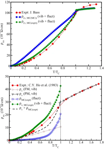
FIG. 8. (Color online) Top: Temperature-dependent longitudinal resistivity of bcc Fe ρ(T) obtained by accounting for ther- mal vibrations and spin fluctuations using the scheme MC vib+fluct[MC(MC)],squares and a mean-field fit to the experi- mental temperature magnetic momentMexpt{vib+fluct[MC(expt)], diamonds}, compared with experimental data (circles) [65]. Bottom:

Corresponding results for fcc Ni. In addition results are shown accounting for thermal displacements (vib) only for the ferromagnetic (FM) and the paramagnetic (PM) regimes. The dashed line represents the sum of resistivities contributed by lattice vibrations or spin fluctuations only. Experimental data have been taken from Ref. [68].

displacements and spin fluctuations using the MC scheme [ρv,MC(MC)(T)] are compared in Fig.8(top) with experimental data [ρexpt(T)]. For the Curie temperature obviously a very good agreement with experiment is found, while for lower temperatures ρ_v,MC(MC)(T) exceeds ρ_expt(T). This behavior correlates well with that of the temperature-dependent reduced magnetic momentM(T) shown in Fig. 3 (middle). The too rapid decrease ofM_MC(T) compared with the experimental results implies an essentially overestimated spin disorder at any temperature, leading in turn to a too large resistivity ρ_v,MC(MC)(T). On the other hand, using the temperature depen- dence of the experimental reduced magnetic momentM_expt(T) to set up the temperature dependent spin configuration as described above a very satisfying agreement ofρ_v,MC(expt)(T) is found with the experimental resistivity dataρ_expt(T). Note also that aboveTCthe calculated resistivity increases the saturation,

in contrast to the experimental data, where the continuing increase ofρ_expt(T) can be attributed to the longitudinal spin fluctuations leading to a temperature-dependent distribution of local magnetic moments on Fe atoms [57]. However, this contribution was not taken into account because of the restriction in present calculations of using fixed values for the local reduced magnetic moments.

Figure 8 (bottom) shows corresponding results for the temperature-dependent resistivity of fcc Ni ( Debye=375 K).

For the ferromagnetic regime that the theoretical results are comparable in magnitude when only thermal displacements [ρv(T)] or only spin fluctuations [ρMC(expt)(T)] are accounted for. In the latter case the mean-field w(T) has been fitted to the experimental M(T) curve. Taking both into account leads to a resistivity [ρ_v,MC(expt)(T)] that is well above the sum of the individual terms ρ_v(T) and ρ_MC(expt)(T). Comparing ρ_v,MC(expt)(T) with experimental data ρ_expt(T), our finding shows that the theoretical results overshoot the experimental ones as one comes closer to the critical temperature. This is a clear indication that the assumption of a rigid spin moment is quite questionable as the resulting contribution to the resistivity due to spin fluctuations as much too small. In fact the simulations of Ruban et al. [57] on the basis of a longitudinal spin fluctuation Hamiltonian led on the case of fcc Ni to a strong diminishing of the average local magnetic moment when the critical temperature is approached from below (about 20% compared to the value atT =0 K). For bcc Fe, the change is much smaller (about 3%) justifying in this case the assumption of a rigid spin moment. Taking the extreme point of view that the spin moment vanishes completely above the critical temperature or in the paramagnetic regime only thermal displacements have to be considered as a source for the finite resistivity. Corresponding results are shown in Fig.8 (bottom) together with corresponding experimental data. The very good agreement between the two obviously suggests that

0 200 400 600 800

Temperature (K) 0

2 4 6 8

α × 103

fluct: MC(MC) fluct: MC(expt) fluct: DLM(expt) fluct: cone(expt)

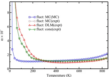
FIG. 9. (Color online) Temperature-dependent Gilbert damping parameterα(T) for bcc Fe obtained by accounting for spin fluctu- ations based on the experimentalM(T) dependence and calculated using the schemes MC (circles), DLM (up triangles), and cone (down triangles); as well as the Gilbert damping parameter calculated by accounting for spin fluctuations using the scheme MC and based on theM(T) dependence obtained in MC simulations.

remaining spin fluctuations above the critical temperature are of minor importance for the resistivity of fcc Ni.

B. Temperature-dependent Gilbert damping parameter Figure9shows results for the Gilbert damping parameter α of bcc Fe obtained using different models for the spin fluctuations. All the curves show the typical conductivitylike behavior for low temperatures and the resistivitylike behavior at high temperatures, reflecting the change from dominating intra- to interband transitions [11]. The curve denoted “expt” is based on a spin configuration obtained from the experimental M_expt(T) data. Using the conical model to fitM_expt(T) as the basis for the calculation ofα(T) leads obviously to a rather good agreement with α_M(expt)(T). With instead a DLM-like representation ofM_expt(T), on the other hand, the transverse spin components are suppressed and noteworthy deviations from α_M(expt)(T) are found for the low-temperature regime.

Nevertheless, the deviations are less pronounced than in the case of the longitudinal resistivity [see Fig. 7 (bottom)],

0 200 400 600 800

Temperature (K) 0

2 4 6 8 10

α × 103

vibvib + fluct(MC(expt)) Expt 1

Expt 2

0 100 200 300 400 500

Temperature (K) 0

0.05 0.1 0.15 0.2

α

vibfluct(MC(Expt)) vib + fluct(MC(Expt)) Expt

FIG. 10. (Color online) Top: Temperature-dependent Gilbert damping α(T) for bcc Fe, obtained by accounting for thermal vibrations and spin fluctuations accounting for lattice vibrations only (circles) and lattice vibrations and spin fluctuations based on a mean-field fit to the experimental temperature-reduced magnetic momentMexpt(diamonds) compared with experimental data (dashed and full lines) [69,70]. Bottom: Corresponding results for fcc Ni.

Experimental data have been taken from Ref. [69].

where corresponding results are shown based onM_MC(T) as a reference. Obviously, the damping parameterαseems to be less sensitive to the specific spin fluctuation model used than the resistivity. Finally, using the spin configuration deduced from Monte Carlo simulations, i.e., based onM_MC(T), quite strong deviations for the resultingα_M(MC)(T) fromα_M(expt)(T) are found. As for the resistivity [see Fig.7(bottom)] this seems to reflect the too fast drop of the reduced magnetic moment M_MC(T) with temperature in the low-temperature regime compared with the drop in temperature (see Fig.3). As was found before [19], accounting only for thermal vibrationsα(T) [Fig.7 (bottom)] gives results comparable to the case when only thermal spin fluctuations are allowed. Combing both thermal effects does not lead to a curve that is just the sum of the twoα(T) curves. As found for the conductivity [Fig.7(top)]

obviously the two thermal effects are not simply additive. As Fig. 10(top) shows, the resulting damping parameter α(T) for bcc Fe that accounts for thermal vibrations as well as spin fluctuations is found to be in reasonable good agreement with experimental data [19].

Figure10shows also corresponding results for the Gilbert damping of fcc Ni as a function of temperature. Accounting only for thermal spin fluctuations on the basis of the experi- mentalM(T) curve leads in this case to completely unrealistic results, while accounting only for thermal displacements leads to results already in rather good agreement with experiment.

Taking finally both sources of disorder into account, again no simple additive behavior is found but the results are nearly unchanged compared to those based on the thermal displacements alone. This implies that the results for the Gilbert damping parameter of fcc Ni hardly depend on the spin fluctuations but are governed significantly by thermal displacements.

V. SUMMARY

Various schemes based on the alloy analogy that allow in- clusion of thermal effects when calculating response properties relevant in spintronics have been presented and discussed.

Technical details of implementation within the framework of the spin-polarized relativistic KKR-CPA band structure method have been outlined that allow thermal vibrations as well as spin fluctuations to be dealt with. Various models to represent spin fluctuations have been compared with each other concerning the corresponding results for the temper- ature dependence of the reduced magnetic moment M(T) as well as response quantities. It was found that response quantities are much more sensitive to the spin fluctuation model than the reduced magnetic momentM(T). Furthermore, it was found that the influence of thermal vibrations and spin fluctuations is not additive when calculating electrical conductivity or the Gilbert damping parameter α. Using experimental data for the reduced magnetic moment M(T) to set up realistic temperature-dependent spin configurations, satisfying agreement for the electrical conductivity as well as the Gilbert damping parameter could be obtained for the elemental ferromagnets bcc Fe and fcc Ni.

ACKNOWLEDGMENTS

Helpful discussions with Josef Kudrnovsk´y and Ilja Turek are gratefully acknowledged. This work was supported fi- nancially by the Deutsche Forschungsgemeinschaft (DFG) within the Projects No. EB154/20-1, No. EB154/21-1, and No. EB154/23-1 as well as the priority program SPP 1538 (Spin Caloric Transport) and the SFB 689 (Spinph¨anomene in Reduzierten Dimensionen).

[1] T. Holstein,Ann. Phys. (NY)29,410(1964).

[2] G. D. Mahan, Many-Particle Physics, Physics of Solids and Liquids (Springer, New York, 2000).

[3] P. B. Allen,Phys. Rev. B3,305(1971).

[4] K. Takegahara and S. Wang,J. Phys. F: Met. Phys. 7,L293 (1977).

[5] G. Grimvall,Phys. Scr.14,63(1976).

[6] G. D. Mahan and W. Hansch,J. Phys. F: Met. Phys.13,L47 (1983).

[7] M. Oshita, S. Yotsuhashi, H. Adachi, and H. Akai,J. Phys. Soc.

Jpn.78,024708(2009).

[8] K. Shirai and K. Yamanaka, J. Appl. Physics 113, 053705 (2013).

[9] D. Steiauf and M. F¨ahnle,Phys. Rev. B72,064450(2005).

[10] V. Kambersk´y,Phys. Rev. B76,134416(2007).

[11] K. Gilmore, Y. U. Idzerda, and M. D. Stiles,Phys. Rev. Lett.99, 027204(2007).

[12] V. Kambersky,Czech. J. Phys.26,1366(1976).

[13] D. Thonig and J. Henk,New J. Phys.16,013032(2014).

[14] P. B. Allen, T. P. Beaulac, F. S. Khan, W. H. Butler, F. J. Pinski, and J. C. Swihart,Phys. Rev. B34,4331(1986).

[15] S. Y. Savrasov and D. Y. Savrasov,Phys. Rev. B 54, 16487 (1996).

[16] B. Xu and M. J. Verstraete,Phys. Rev. B87,134302(2013).

[17] B. Xu and M. J. Verstraete,Phys. Rev. Lett.112,196603(2014).

[18] Y. Liu, A. A. Starikov, Z. Yuan, and P. J. Kelly,Phys. Rev. B84, 014412(2011).

[19] H. Ebert, S. Mankovsky, D. K¨odderitzsch, and P. J. Kelly,Phys.

Rev. Lett.107,066603(2011).

[20] J. Braun, J. Min´ar, S. Mankovsky, V. N. Strocov, N. B. Brookes, L. Plucinski, C. M. Schneider, C. S. Fadley, and H. Ebert,Phys.

Rev. B88,205409(2013).

[21] J. Kudrnovsk´y, V. Drchal, I. Turek, S. Khmelevskyi, J. K.

Glasbrenner, and K. D. Belashchenko,Phys. Rev. B86,144423 (2012).

[22] J. K. Glasbrenner, K. D. Belashchenko, J. Kudrnovsk´y, V. Drchal, S. Khmelevskyi, and I. Turek, Phys. Rev. B85, 214405(2012).

[23] R. Kov´aˇcik, P. Mavropoulos, D. Wortmann, and S. Bl¨ugel,Phys.

Rev. B89,134417(2014).

[24] S. Mankovsky, D. K¨odderitzsch, and H. Ebert (unpublished).

[25] H. Akai and P. H. Dederichs,Phys. Rev. B47,8739(1993).

[26] A. I. Liechtenstein, M. I. Katsnelson, V. P. Antropov, and V. A.

Gubanov,J. Magn. Magn. Mater.67,65(1987).

[27] B. L. Gyorffy, A. J. Pindor, J. Staunton, G. M. Stocks, and H. Winter,J. Phys. F: Met. Phys.15,1337(1985).

[28] B. Velick´y,Phys. Rev.184,614(1969).

[29] W. H. Butler,Phys. Rev. B31,3260(1985).

[30] S. Lowitzer, M. Gradhand, D. K¨odderitzsch, D. V. Fedorov, I.

Mertig, and H. Ebert,Phys. Rev. Lett.106,056601(2011).

[31] A. Brataas, Y. Tserkovnyak, and G. E. W. Bauer,Phys. Rev.

Lett.101,037207(2008).

[32] D. K¨odderitzsch, K. Chadova, J. Min´ar, and H. Ebert,New J.

Phys.15,053009(2013).

[33] A. Cr´epieux and P. Bruno,Phys. Rev. B64,094434(2001).

[34] J. S. Faulkner and G. M. Stocks, Phys. Rev. B 21, 3222 (1980).

[35] P. Weinberger, Electron Scattering Theory for Ordered and Disordered Matter(Oxford University Press, Oxford, 1990).

[36] H. Ebert, in Electronic Structure and Physical Properties of Solids, edited by H. Dreyss´e, Lecture Notes in Physics Vol. 535 (Springer, Berlin, 2000), p. 191.

[37] S. Lowitzer, D. K¨odderitzsch, and H. Ebert,Phys. Rev. Lett.

105,266604(2010).

[38] M. E. Rose,Relativistic Electron Theory (Wiley, New York, 1961).

[39] I. Turek, J. Kudrnovsk´y, V. Drchal, L. Szunyogh, and P.

Weinberger,Phys. Rev. B65,125101(2002).

[40] J. B. Staunton and B. L. Gyorffy,Phys. Rev. Lett.69,371(1992).

[41] M. Jonson and G. D. Mahan,Phys. Rev. B42,9350(1990).

[42] S. Mankovsky, D. K¨odderitzsch, G. Woltersdorf, and H. Ebert, Phys. Rev. B87,014430(2013).

[43] H. B¨ottger, Principles of the Theory of Lattice Dynamics (Akademie-Verlag, Berlin, 1983).

[44] E. M. Gololobov, E. L. Mager, Z. V. Mezhevich, and L. K. Pan, Phys. Status Solidi B119,K139(1983).

[45] E. Francisco, M. A. Blanco, and G. Sanjurjo,Phys. Rev. B63, 094107(2001).

[46] N. Papanikolaou, R. Zeller, P. H. Dederichs, and N. Stefanou, Phys. Rev. B55,4157(1997).

[47] A. Lodder,J. Phys. F: Met. Phys.6,1885(1976).

[48] L. Udvardi, L. Szunyogh, K. Palot´as, and P. Weinberger,Phys.

Rev. B68,104436(2003).

[49] H. Ebert and S. Mankovsky,Phys. Rev. B79,045209(2009).

[50] S. Mankovsky, S. Polesya, H. Ebert, W. Bensch, O. Mathon, S.

Pascarelli, and J. Min´ar,Phys. Rev. B88,184108(2013).

[51] M. Pajda, J. Kudrnovsk´y, I. Turek, V. Drchal, and P. Bruno, Phys. Rev. B64,174402(2001).

[52] S. Tikadzumi,Physics of Magnetism, (Willey, Ney York, 1964).

[53] H. Akai,Phys. Rev. Lett.81,3002(1998).

[54] J. B. Staunton, S. Ostanin, S. S. A. Razee, B. L. Gyorffy, L. Szunyogh, B. Ginatempo, and E. Bruno, Phys. Rev. Lett.

93,257204(2004).

[55] J. Crangle and G. M. Goodman, Proc. R. Soc. London, Ser. A321,477(1971),http://rspa.royalsocietypublishing.org/

content/321/1547/477.full.pdf+html.

[56] S. V. Halilov, H. Eschrig, A. Y. Perlov, and P. M. Oppeneer, Phys. Rev. B58,293(1998).

[57] A. V. Ruban, S. Khmelevskyi, P. Mohn, and B. Johansson,Phys.

Rev. B75,054402(2007).

[58] V. Drchal, J. Kudrnovsk´y, and I. Turek,EPJ Web Conf.40, 11001(2013).

[59] V. Drchal, J. Kudrnovsk´y, and I. Turek,J. Supercond. Novel Magn.26,1997(2013).

[60] J. B. Staunton, R. Banerjee, M. dos Santos Dias, A. Deak, and L. Szunyogh,Phys. Rev. B89,054427(2014).

[61] H. Ebert, D. K¨odderitzsch, and J. Min´ar,Rep. Prog. Phys.74, 096501(2011).

[62] H. Ebertet al., The Munich SPR-KKR Package, version 6.3, http://olymp.cup.uni-muenchen.de/ak/ebert/SPRKKR(2012).

[63] S. H. Vosko, L. Wilk, and M. Nusair,Can. J. Phys.58,1200 (1980).

[64] D. K¨odderitzsch, S. Lowitzer, J. B. Staunton, and H. Ebert,Phys.

Status Solidi B248,2248(2011).

[65]Electrical Resistivity of Pure Metals and Alloys, edited by J.

Bass, Landolt-Bornstein, New Series, Group III, Vol. 15, Pt. A (Springer, New York, 1982).

[66] J. Banhart, H. Ebert, P. Weinberger, and J. Voitl¨ander,Phys. Rev.

B50,2104(1994).

[67] I. Turek, J. Kudrnovsk´y, V. Drchal, and P. Weinberger,J. Phys.:

Condens. Matter16,S5607(2004).

[68] C. Y. Ho, M. W. Ackerman, K. Y. Wu, T. N. Havill, R. H.

Bogaard, R. A. Matula, S. G. Oh, and H. M. James,J. Phys.

Chem. Ref. Data12,183(1983).

[69] S. M. Bhagat and P. Lubitz,Phys. Rev. B10,179(1974).

[70] B. Heinrich and Z. Frait,Phys. Status Solidi B16,1521(1966).