Calculating Joint Confidence Bands for Impulse Response Functions using Highest Density Regions

SFB 649 Discussion Paper 2016-017

Calculating Joint Confidence Bands for

Impulse Response Functions using

Highest Density Regions Helmut Lütkepohl*

Anna Staszewska-Bystrova*² Peter Winker*³

* DIW Berlin and Freie Universität Berlin, Germany

* University of Lodz, Poland

* University of Giessen, Germany

This research was supported by the Deutsche

Forschungsgemeinschaft through the SFB 649 "Economic Risk".

http://sfb649.wiwi.hu-berlin.de ISSN 1860-5664

SFB 649, Humboldt-Universität zu Berlin

SFB

6 4 9

E C O N O M I C

R I S K

B E R L I N

Calculating Joint Confidence Bands for Impulse Response Functions using Highest

Density Regions

Helmut L¨ utkepohl

DIW Berlin and Freie Universit¨at Berlin Mohrenstr. 58

10177 Berlin, Germany email: hluetkepohl@diw.de

Anna Staszewska-Bystrova

University of Lodz Rewolucji 1905r. 41 90-214 Lodz, Poland email: emfans@uni.lodz.pl

Peter Winker

University of Giessen Licher Str. 64 35394 Giessen, Germany

email: Peter.Winker@wirtschaft.uni-giessen.de March 15, 2016

Abstract

This paper proposes a new non-parametric method of constructing joint con- fidence bands for impulse response functions of vector autoregressive models.

The estimation uncertainty is captured by means of bootstrapping and the highest density region (HDR) approach is used to construct the bands. A Monte Carlo comparison of the HDR bands with existing alternatives shows that the former are competitive with the bootstrap-based Bonferroni and Wald confidence regions. The relative tightness of the HDR bands matched with their good coverage properties makes them attractive for applications.

An application to corporate bond spreads for Germany highlights the poten- tial for empirical work.

Key Words: Impulse responses, joint confidence bands, highest density re- gion, vector autoregressive process

JEL classification: C32

1 Introduction

During the last few years, a substantial number of methods for construct- ing joint confidence bands for impulse response functions (IRFs) of vector autoregressive (VAR) models has been proposed. Adding to previous ap- proaches based on asymptotic considerations, the more recent proposals are based on bootstrap methods to obtain a better approximation for the sample sizes typically considered in applied macroeconomic studies. For an overview and comparison of these methods see L¨utkepohl et al. (2015a, 2015b) and the papers cited therein.

Several of the bootstrap based methods have been shown in Monte Carlo studies to outperform asymptotic methods and the simplified approach of constructing the bands pointwise. The actual coverage of the bands is found to be closer to the nominal level for these methods. In particular, L¨utkepohl et al. (2015b) found that Bonferroni based methods are competitive with other more refined methods, although – as expected – they provide exces- sively conservative bands. Taking into account the dependency over the horizon of impulse response functions relying on a Wald type approach did not improve the properties of the regions. One of the reasons for this a priori unexpected result is seen in the given geometric form of the Wald ellipse in the parameter space, which has to be mapped to a multidimensional box in the space of the IRFs corresponding to the bands.

As an alternative to the parametric Wald approach, the construction of a set of IRFs might be tackled directly in a non-parametric way. In this paper, we use the highest density region (HDR) approach proposed by Hyndman (1995, 1996) and also discussed in the context of VAR analysis in Fresoliet al.

(2015). In contrast to the Wald approach, for this non-parametric method, the scaling of the variables or error terms, respectively, might influence the outcome. Consequently, for our analysis we consider both a straightforward implementation of the HDR method and two versions including different versions of a scaling step.

The paper is structured as follows. Section 2 presents the model and selected existing methods of constructing confidence bands for impulse re- sponses. In Section 3, we describe the proposed non-parametric method and how it relates to the benchmark approaches. The relative performance of the method is analyzed by means of a Monte Carlo study. Section 4 provides the setup and results of this analysis. An application to the modeling of corporate bond spreads highlights that the choice of an appropriate method might also affect qualitative conclusions. The application and estimation re- sults are presented in Section 5. Finally, Section 6 provides a summary of the main findings and an outlook to future research.

2 Inferences about Impulse Response Func- tions

The methods proposed in the literature for constructing joint bands for IRFs might be classified into three groups. First, there are methods relying on asymptotic considerations (e.g., Jord`a (2009) and Staszewska-Bystrova (2013)). These methods have been shown to exhibit an unsatisfactory per- formance for typical sample sizes.¹ A second group of methods relies on the bootstrap to approximate the distribution of the estimators. Then, classical methods for joint inference are used to construct the bands (see L¨utkepohl et al. (2015b) and Inoue and Kilian (2016)). L¨utkepohlet al.(2015a) present simulation evidence on these two approaches. Given that traditional meth- ods, e.g., based on Bonferroni’s inequality might result in too conservative, i.e., excessively wide bands, in a third class of methods, the focus of the construction procedures is on the width of the bands. However, explicit opti- mization methods as the ones presented in Staszewska-Bystrova and Winker (2013) for the case of the related problem of constructing prediction bands come at substantial computational cost and tend to be too aggressive, i.e., tend to produce bands with an actual coverage below the nominal level.

While further research is required to better understand the reasons for the shortcomings of the existing methods, which might help to adjust them in an appropriate way, a distinct approach of constructing highest density bands is followed in this paper.

Before presenting the method in Section 3 below, we first describe the impulse responses of structural VARs and two approaches to constructing confidence bands used as benchmarks in the Monte Carlo study.

2.1 Impulse Response Analysis

In the following we consider a K-dimensional reduced form VAR(p) process:

y_t=ν+A₁y_t−1 +· · ·+A_py_t−p+u_t, u_t∼(0,Σ_u), (2.1) where A_i for i = 1, . . . , p, are square parameter matrices of order K, ν represents a vector of intercepts and the reduced form errors, u_t, are an independent white noise process. Possible other deterministic terms, like a trend or appropriate dummy variables are neglected as they are not relevant for the methods discussed below.

If the stability condition, i.e.,

detA(z) = det(I_K−A₁z− · · · −A_pz^p)6= 0 for z ∈C,|z| ≤1, (2.2) is met, the process can be represented as a moving average:

y_t=µ+

∞

X

i=0

Φ_iu_t−i, (2.3)

1See, e.g., Staszewska-Bystrova and Winker (2013).

where µ = (IK −A1 −. . .−Ap)⁻¹ν, Φ0 = IK and Φi = Pi

j=1Φi−jAj for i= 1,2, . . . (L¨utkepohl 2005, p. 23).

Uncorrelated structural innovations with zero means and unit variances are often obtained from the reduced form errors as εt =B⁻¹ut, where B is the matrix of impact effects. In order to identify B, at least K(K −1)/2 restrictions have to be imposed. If justified, this can be achieved, e.g. by assuming a recursive structure of the variables, that is by obtaining a lower triangular matrix Bfrom a Cholesky decomposition of Σ_u. In the paper we focus on this identification scheme, however all the methods are applicable also for other sets or types of identifying restrictions. Responses to structural shocks can be found from (2.3) by replacing u_t with Bε_t,

y_t=µ+

∞

X

i=0

Φ_iBεt−i =µ+

∞

X

i=0

Θ_iεt−i. (2.4)

Our interest is in the impulse responses Θ_i = Φ_iB, i= 0,1, . . ..

Inferences on the structural impulse responses are performed as follows.

Estimation of ν, A₁, . . . , A_p is done using multivariate ordinary least squares with the bias-correction based on a closed form bias formula presented by Nicholls and Pope (1988). If the bias-correction causes nonstationarity (as compared to the system estimated by OLS), the stationarity correction de- scribed by Kilian (1998) and consisting in reducing the value of bias esti- mates, is applied. The residuals are used to compute an estimate of Σ_u. These estimators are denoted by bν,Ab₁, . . . ,Ab_p and Σb_u. If a model selec- tion step is performed, the lag length pis chosen on the basis of the Akaike information criterion (AIC). The estimates for the impulse responses for an assumed propagation horizonH are computed as functions ofAb₁, . . . ,Ab_p and Σb_u and denoted by Θb₀,Θb₁, . . . ,Θb_H.

The methods for constructing confidence bands are based on standard residual-based bootstraps (for details see, e.g., L¨utkepohl et al. (2015a)).

Application of the bootstrap method results in N replicates of Ab₁, . . . ,Ab_p and Σb_u, denoted by Abⁿ₁, . . . ,Abⁿ_p,Σbⁿ_u and the same number of replicates of Θb₀,Θb₁, . . . ,Θb_H, denoted byΘbⁿ₀,Θbⁿ₁, . . . ,Θbⁿ_H for n = 1, . . . , N.

2.2 Benchmark Methods for Constructing Joint Con- fidence Bands

In the Monte Carlo simulations, we compare the HDR bands with two bench- marks. The alternatives are: the bootstrap-based Bonferroni band and the Wald band considered, e.g., by L¨utkepohlet al.(2015b). These methods have been shown to have coverage levels for impulse responses that usually exceed the nominal level, but are often quite close to it. The drawback of the bands is their large width, which is especially true for the Wald band. Excessive width is a problem, as it implies that the band becomes less informative about the true shape of the response function.

The Bonferroni band, denoted by B, computed for the nominal confidence level of 1−γ is obtained by forming intervals with appropriately adjusted

coverage rates for individual values of the response function of interest. For the response of thej-th variable to thek-th shock, the band is calculated as:

[B_jk,0^l , B_jk,0^u ]×[B_jk,1^l , B_jk,1^u ]× · · · ×[B_jk,H^l , B_jk,H^u ],

where B_jk,h^l and B_jk,h^u for h= 0, . . . , H are the γ/2(H+ 1) and 1−γ/2(H+ 1) quantiles of the bootstrap distribution of θb_jk,h, where θb_jk,h is the jk-th element of Θb_h. If the effect on impact is zero (by assumption), the interval [B^l_jk,0, B_jk,0^u ] is not formed and the remaining intervals forh= 1, . . . , H have nominal coverage rates of 1−γ/H.

The Wald band is based on the bootstrapped Wald statistic formulated with respect to the VAR parameters. For δ denoting the vector of VAR coefficients A₁, . . . , A_p and the appropriate parameters from the matrix B, the method relies on the following asymptotic result:

√

T(bδ−δ)→N^d (0,Σδ), (2.5)

where T is the sample size.

Computation of the Wald band (W) for the response of variablej to shock k and confidence level of 1−γ, involves the following steps:

1. For the bootstrap replication n= 1, . . . , N, obtain wⁿ=T(bδⁿ−bδ)⁰Σbδ(n)⁻¹(bδⁿ−bδ), and Θbⁿ₀,Θbⁿ₁, . . . ,Θbⁿ_H.

2. Find wⁿ_1−γ, denoting the (1−γ) quantile of the bootstrapped values wⁿ and select θbⁿ_jk,0, . . . ,θbⁿ_jk,H obtained in bootstrap replications with wⁿ < wⁿ_1−γ.

3. Form the band

[W_jk,0^l , W_jk,0^u ]×[W_jk,1^l , W_jk,1^u ]× · · · ×[W_jk,H^l , W_jk,H^u ],

by finding the smallest and the largest values from the selected bθⁿ_jk,h for each h= 0, . . . , H.

3 Using Highest Density Regions

The proposed method exploits ideas from non-parametric modeling of mul- tivariate distributions. The starting point is a set of IRFs obtained from N bootstrap replications for horizon H. The aim is to find a hyperrectangle in the (H+ 1)-dimensional space which is not excessively large and comprising at least (1−γ)N elements, where 1−γis the nominal coverage level.² In order to reach this goal, it appears natural to focus on those areas, where a high

2If the response on impact is restricted to 0, the dimension of the analysis is given by H instead ofH+ 1.

concentration of the generated points can be found, and to neglect points which are rather far off. Obviously, an operationalization of this concept is not straightforward in higher dimensions.

In Fresoli et al. (2015), the authors use highest density regions to illus- trate the joint predictive distribution for two variables. The method has been proposed by Hyndman (1996). Fresoli et al. conclude that this method is infeasible in higher dimensions. In fact, the actual estimation of the multi- variate density function and the derived highest density region would require a huge number of points when the dimensions grow beyond three or four. In the application to IRFs, the dimension is given by the horizon considered for a single IRF, and by a multiple of this horizon if several IRFs are considered jointly. Thus, the actual dimension might be rather large. In principle, given that the number of bootstrap replications N can go to infinity even for a small data set, this constraint might not be considered as binding. However, in order to estimate precisely a multivariate density, e.g., in dimension 10 or 20, the number of replications required becomes too large given available computational resources.

Nevertheless, a non-parametric estimate of the density for each of the generated bootstrap vectors (IRFs) can be calculated at rather low compu- tational cost. Furthermore, for the construction of bands, it is not required to identify the highest density region as a whole, but to find a hyperrectan- gle covering a share of (1−γ) of the density. Instead of constructing this hyperrectangle from the approximated density function, it will be obtained directly from the bootstrap replications by selecting the (1−γ)N generated points with highest density and the construction of the smallest rectangular box including all these points. This box corresponds to a band in the time dimension, which is labeled HDR-band in the following.

The construction of HDR-bands consists of the following steps:

1. Given a matrixDof dimensions N×(H+ 1) corresponding toN boot- strap replicates of a (H+ 1)-dimensional vector (each corresponding to an IRF), calculate the N×N matrix E of pairwise squared Euclidean distances.

2. Let ˆs = q 1

H+1

PH+1

i=1 var(D_.,i) be the square root of the mean of the variances across dimensions; it is considered as a proxy of the variation in each dimension used to obtain a bandwidth estimator for the kernel density estimates.

3. The bandwidth h^S according to Scott’s rule for a multivariate normal distribution (Scott 1992, p. 152) is given by

h^S = ˆsN^−H+51 .

For alternative distributional assumptions, different bandwidths might be selected. However, preliminary experiments show that the effect on the HDR-band are rather negligible unless the bandwidth is changed by an order of magnitude.

4. The density estimate for each single bootstrap replication i (row of matrix D) is obtained by

di = 1 N(h^S)^H+1

N

X

n=1

1

(2π)^(H+1)/2e^{−2hS1 Ein}.

5. For a given confidence level 1−γ, the points with highest density are obtained by excluding the γN points with the lowest density values.³ 6. The hyperrectangle corresponding to the HDR-band is obtained by us-

ing the minimum and maximum of the included highest density points in each dimension. Obviously, if all these points are included in the box, their convex hull is also included.

For illustrating the method, we start with a simplified setting, where the known distribution is given by a two-dimensional standard normal distri- bution with (auto)correlation of ρ = 0.8. Figure 1 shows the outcome of a Monte Carlo simulation, drawing N = 2 000 realizations from the given distribution. As nominal coverage level, we set (1−γ) = 0.95.

The figure shows the simulated data points (which would correspond to one IRF over two periods each for the application in the VAR setting). The grey shaded points are those with the highest non-parametric density esti- mates (their number is given by 1900 = (1−γ)N), while the black points are the excluded points with low density. The black dot-dashed line shows the smallest rectangular box containing all the highest density points, i.e., it corresponds to the HDR-band. For comparison purposes, we also show the boxes constructed following alternative methods. First, the box labeled as

“na¨ıve” (dotted lines) is given by a centered 1−γ interval for each dimension separately. It becomes obvious by visual inspection that its actual coverage might be too low. The Bonferroni band (solid black lines) is obtained by using centered 1−γ/2 intervals for each dimension separately in order to guarantee a coverage of at least 1−γ, while the Wald band (grey dashed lines) results from determining the smallest hyperrectangle comprising the 1−γ central confidence ellipse (grey) based on the Wald statistic.⁴

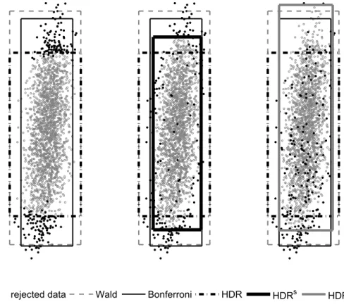
The straightforward implementation of the method as described above seems to give sensible results for the simplified situation of a multivariate normal distribution with equal variances across dimensions. If those vari- ances differ substantially as is typically the case for IRFs, the quality of the approximation might deteriorate as indicated by the example shown in the left panel of Figure 2. The data points in this figure correspond to boot- strapped IRFs of length 11 (horizon 10 plus initial response) of the first variable to the first shock generated from a two dimensional VAR introduced

3Note that for the construction of the HDR-band, an explicit definition of a highest density region (HDR) is not required. A natural candidate would be the convex hull of the highest density points.

4For some arguments explaining the larger size of the Wald band as compared to the Bonferroni band, see L¨utkepohlet al. (2015b).

−3.5 0 3.5

−3.5 0 3.5

rejected data naive Wald Bonferroni HDR Figure 1: Comparison of alternative confidence sets for a 2-dimensional nor- mal distribution

in Section 4 with ϕ = 0.9. The projection is done for horizons h = 0 and h= 6 and the confidence level is set to 0.9.

In order to avoid a bias stemming from differences in variances or specific covariance structures, either the non-parametric estimator might be adjusted, e.g., by using the actual standard deviation per dimension instead of identical values for all dimensions, or the data have to be standardized prior to the application of the HDR method. The latter is the approach followed here making use of two different strategies.

The first strategy focuses only on the standard deviations. Consequently, prior to the application of the algorithm for the construction of HDR bands, the bootstrapped values are standardized by the bootstrap standard devia- tion for each horizon. After the calculation of the HDR band, the resulting values are multiplied with the same standard deviation mapping the band back to the original space. This improved HDR band, which might be more appropriate in situations with substantially differing standard deviations of IRFs across horizons, is labeled HDR^s in the following. The middle panel in Figure 2 shows the impact on the form of the band taking into account the higher variance for the second horizon and thereby achieving a more even

rejected data Wald Bonferroni HDR HDR^s HDR^w

Figure 2: Comparison of alternative bands for an IRF from bivariate VAR

rejection of data points with regard to both horizons shown in the projection.

A second strategy takes into account the full variance-covariance matrix of the bootstrapped values. In the first step, the bootstrapped IRFs are whitened and then used in the search of the highest density region. After rejecting the required number of bootstrap vectors, the reverse transforma- tion is applied with respect to the retained vectors to restore their original values. The band obtained using the bootstrap IRFs selected in this way is denoted by HDR^w and illustrated, for the example considered in Figure 2, in the right hand panel. It can be seen that the HDR^w band is similar to the HDR^s region in rejecting data points for both horizons, but is larger than the latter region.

The detailed steps used in the computation of HDR^s and HDR^w bands are as follows.

1. Compute a bootstrap estimate of the variance matrix of impulse re- sponses, Ω, using the shrinkage estimator (Ledoit and Wolf 2003):e

Ω =e λdiag(bω11, . . . ,ωbH+1,H+1) + (1−λ)bΩ,

where Ω is an unbiased bootstrap estimator of the covariance ma-b trix with element ij computed as: ωb_ij = _N¹₋₁ PN

n=1vⁿ_ij, where vⁿ_ij = (d_ni−d_i)(d_nj−d_j) andd_ni is theni-th element of matrix D. diag(ωb₁₁, . . . ,bω_H+1,H+1) denotes a diagonal matrix whose main diagonal is the same as in Ω.b

2. For the HDR^s method set λ= 1.

3. For the HDR^w method estimateλas proposed by Sch¨afer and Strimmer (2005) for the case of a diagonal target matrix with unequal variances:

bλ= P

i6=jvar(d ωb_ij) P

i6=jbω²_ij ,

where var(d ωb_ij) stands for the unbiased variance estimator of the indi- vidual element of Ω calculated as:b

var(d ωb_ij) = N (N −1)³

N

X

n=1

(v_ijⁿ −v_ij)².

4. Perform the Cholesky decomposition: Ω =e LL⁰and transform the boot- strap paths: D(L⁰)⁻¹.

5. Apply the algorithm for constructing the HDR bands to the trans- formed paths to reject γN paths.

6. Denote the matrix containing the remaining paths as DHDR, compute D_HDRL⁰ and construct the band by finding the smallest and largest values for each horizon.

Obviously, the proposed HDR approaches allow for further modifications.

In particular, a more refined analysis of the impact of the choice of kernel functions and bandwidth selection could be of interest. Furthermore, sim- ilar adjustments as for the variances by HDR^s and the variance-covariance by HDR^w could also be considered with regard to higher moments, e.g., if the distribution of the IRFs turns out to be more heavily skewed at some horizons. Such extensions of the analysis are left for future research.

4 Monte Carlo Analysis

4.1 Monte Carlo Design

For the Monte Carlo analysis, we use the same setting as in L¨utkepohl et al.(2015a, 2015b) and complement it by a substantially larger VAR (both in terms of dimension and lag length) inspired by a real application (Staszewska- Bystrova and Winker 2014).

The first setting (labeled DGP1) consists in a bivariate DGP with one lag taken originally from Kilian (1998). It is given by:

y_t=

ϕ 0 0.5 0.5

y_t−1 +u_t, u_t∼iid N

0,

1 0.3 0.3 1

, (4.1)

where the parameterϕtakes on values in{−0.95,−0.9,−0.5,0,0.5,0.9,0.95,1}.

It determins the persistence of the process. For ϕ = 1, the process is non- stationary, but cointegrated. For a discussion of this special case and the

singularity for ϕ = 0 see L¨utkepohl et al. (2015b). As in previous research, sample sizes used are T = 50,100 and 200. The orthogonal IRFs with hori- zonsH = 10 andH = 20, respectively, are obtained by applying the Cholesky decomposition of the estimated residual covariance matrix imposing a zero constraint on the reaction of the first variable on impact of the second shock.

The second DGP (DGP2) provides some insights on the relative perfor- mance of methods for a substantially more complex VAR model which might be relevant for empirical applications. It is based on the example described in Section 5. The model for German corporate bond spreads includes six variables. Model selection criteria suggest a lag order of four. The rounded estimates of the corresponding 144 parameters describing the dynamics of the DGP, the six constants and the 6×6 variance-covariance matrix are pro- vided in Appendix A. Given the complexity of the model, we consider sample sizes of T = 200 and 400 for horizons H = 12 and H = 24 corresponding to one and two years, respectively. Again, orthogonal impulse responses are calculated (for details see Section 5).

All simulations for both DGPs were done twice: first under the assump- tion that the true lag order is known and used, and second, by selecting the lag order based on Akaike’s information criterion. For the latter approach, the maximum lag length was set as a function of the sample size and the VAR dimension. It is given by 10, 12, and 14 for samples of 50, 100, and 200 observations for DGP1 and by 8 and 10 for sample sizes of 200 and 400 for DGP2. Furthermore, the number of bootstrap replications isN = 2 000, andγ is set to 0.1 corresponding to 90% confidence bands. Finally, for each setting, 2 000 Monte Carlo replications are generated and used for the analysis.

Two features of the confidence bands are evaluated, namely their actual coverage rates with respect to true response functions and their mean widths.

The width is computed by adding the lengths of the intervals around indi- vidual impulse response parameters over the periods from 0 to H.

4.2 Simulation Results

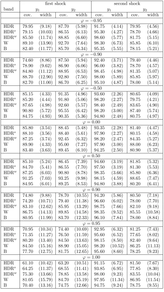
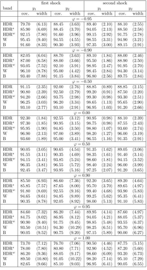
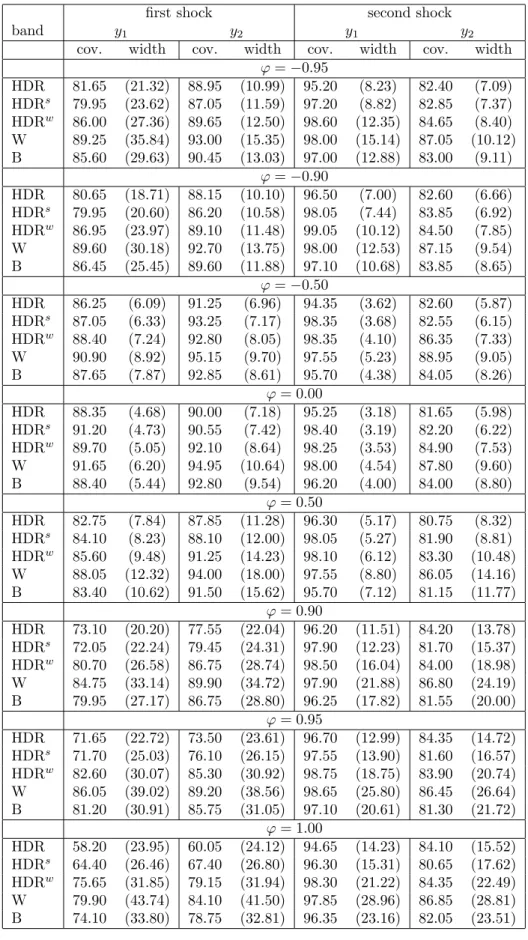
Table 1 summarizes the results forDGP1with T = 50 observations, a horizon for the IRFs of H = 10 and the lag order estimated by Akaike’s information criterion. The results for larger sample sizes and the longer horizon H = 20 are given in Appendix B, while all results forDGP1and the case of known lag order are provided in Appendix C.

Results from Table 1 indicate that for a small sample size of 50 observa- tions no method is able to deliver bands with the expected actual coverage for all the cases. Out of the three HDR methods, the best results in terms of estimated coverage probabilities are obtained for HDR^w, while the HDR and HDR^s bands perform worse and rather similarly. As can be expected, the better coverage properties of HDR^w come at the cost of a larger band width as compared to HDR and HDR^s. HDR^w is also uniformly superior to the traditional Bonferroni method. The HDR^w bands have more precise cov- erage rates accompanied by similar and sometimes even smaller width than the Bonferroni regions. Overall, the best coverage results are obtained by

Table 1: Estimated coverage probabilities and mean widths (in parentheses) of 90% confidence bands for DGP1, T = 50, H = 10 and estimated lag order

first shock second shock

band y₁ y₂ y₁ y₂

cov. width cov. width cov. width cov. width ϕ=−0.95

HDR 79.95 (9.18) 87.70 (5.98) 91.75 (4.14) 79.95 (4.56) HDR^s 79.15 (10.03) 86.55 (6.13) 95.30 (4.27) 78.70 (4.66) HDR^w 85.50 (11.74) 88.85 (6.60) 98.60 (5.77) 81.75 (5.15) W 89.10 (13.90) 92.70 (7.64) 98.30 (6.73) 85.85 (6.10) B 82.40 (11.77) 85.70 (6.34) 95.35 (5.55) 78.15 (5.21)

ϕ=−0.90

HDR 74.60 (8.86) 87.50 (5.94) 92.40 (3.71) 79.40 (4.46) HDR^s 78.90 (9.62) 86.90 (6.06) 96.00 (3.82) 78.70 (4.57) HDR^w 84.80 (11.12) 88.95 (6.53) 98.45 (4.98) 81.35 (5.07) W 88.70 (12.90) 92.80 (7.50) 98.00 (5.89) 85.85 (5.97) B 82.70 (11.00) 86.70 (6.25) 95.10 (4.87) 78.00 (5.14)

ϕ=−0.50

HDR 85.15 (4.33) 91.35 (4.96) 93.60 (2.26) 80.65 (4.09) HDR^s 85.20 (4.44) 91.80 (5.06) 98.20 (2.27) 79.75 (4.21) HDR^w 87.65 (4.98) 92.60 (5.57) 98.40 (2.49) 83.65 (4.90) W 90.80 (5.72) 95.55 (6.42) 98.20 (3.00) 87.40 (5.74) B 84.75 (4.93) 90.35 (5.36) 94.80 (2.48) 80.75 (4.97)

ϕ= 0.00

HDR 85.80 (3.54) 88.45 (5.48) 93.35 (2.28) 81.40 (4.47) HDR^s 88.10 (3.56) 88.40 (5.61) 97.90 (2.27) 80.15 (4.58) HDR^w 87.25 (3.74) 92.45 (6.32) 98.20 (2.47) 84.35 (5.27) W 89.90 (4.33) 95.00 (7.27) 97.90 (3.00) 88.00 (6.23) B 83.40 (3.63) 89.45 (6.10) 94.25 (2.50) 80.90 (5.37)

ϕ= 0.50

HDR 85.10 (5.24) 86.45 (7.39) 94.60 (3.19) 81.85 (5.32) HDR^s 84.70 (5.41) 86.55 (7.70) 97.50 (3.19) 81.30 (5.53) HDR^w 87.25 (6.03) 90.80 (8.78) 98.35 (3.66) 85.80 (6.36) W 91.25 (7.03) 93.25 (9.98) 98.15 (4.59) 88.65 (7.47) B 84.95 (6.01) 89.25 (8.53) 94.80 (3.88) 80.20 (6.41)

ϕ= 0.90

HDR 74.80 (9.88) 78.70 (10.55) 94.20 (5.86) 80.50 (7.18) HDR^s 74.20 (10.71) 79.40 (11.38) 96.60 (6.02) 78.00 (7.70) HDR^w 83.10 (12.62) 85.95 (13.29) 98.75 (7.66) 82.10 (9.18) W 86.75 (14.13) 89.85 (14.58) 98.35 (9.52) 85.55 (10.58) B 80.95 (11.99) 83.70 (12.33) 96.10 (7.84) 78.00 (8.84)

ϕ= 0.95

HDR 70.95 (10.34) 74.40 (10.69) 92.95 (6.32) 81.25 (7.43) HDR^s 71.35 (11.27) 76.50 (11.59) 95.60 (6.52) 77.65 (8.02) HDR^w 80.20 (13.40) 84.50 (13.63) 98.15 (8.50) 82.40 (9.64) W 84.50 (15.16) 88.90 (15.05) 98.20 (10.52) 86.25 (11.13) B 77.70 (12.75) 81.75 (12.65) 95.60 (8.60) 78.25 (9.23)

ϕ= 1.00

HDR 61.10 (10.42) 63.20 (10.51) 91.15 (6.72) 81.50 (7.67) HDR^s 64.25 (11.37) 68.55 (11.41) 93.85 (6.95) 77.85 (8.30) HDR^w 75.30 (13.66) 78.85 (13.58) 98.00 (9.23) 83.55 (10.04) W 81.05 (15.79) 84.70 (15.19) 97.95 (11.34) 86.95 (11.54) B 70.40 (13.16) 74.75 (12.66) 94.75 (9.24) 78.75 (9.55)

the Wald band which is also the widest of all. This inflation of width seems to be justified for the smallest samples analyzed in Table 1.

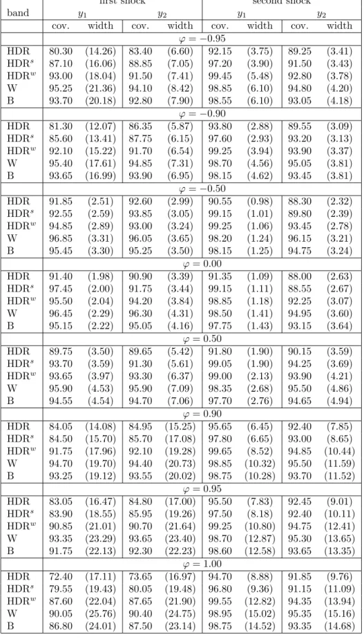
Tables 4–8 in Appendix B show how the conclusions change if larger samples and longer propagation horizons are investigated. First, for larger sample sizes (T = 100 and T = 200) all the coverage probability estimates go up. In effect, the Wald method is no longer best, as both the HDR^w and B bands have more precise coverage rates and are at the same time narrower than the Wald bands. This indicates, that for more realistic sample sizes, the Wald bands are excessively large which is not attractive for empirical applications. Second, for T = 100,200 and H = 10 the dominance of the HDR^w method over the Bonferroni method is less clear than for T = 50, as the coverage probabilities of the two types of bands become more similar.

The HDR^w regions may be still found superior as in many cases they have coverage exceeding 90% and smaller widths. Third, the HDR^w bands gain advantage over the Bonferroni bands as H increases. A longer propagation horizon brings the nominal coverage levels of the intervals making up the Bonferroni band closer to 1, which may result in large width of the B bands.

This can be seen in Tables 7 and 8, where the HDR^w bands are more precise both in terms of coverage and width than the Bonferroni bands. Fourth, the HDR and HDR^s regions perform better for larger T and continue to be the narrowest. However, especially for more persistent processes, their coverage rates may still fall below the nominal level.

The findings are qualitatively almost the same if the true lag order of 1 is used in the simulations (Tables 9–14 in Appendix C). As theoretically justified, given more information on the model, the coverage probabilities increase and the mean width estimates decrease. In effect, the Wald bands become too wide and cease to be competitive even for T = 50.

As a robustness check, we repeated all the simulations for DGP1 without the assumption regarding the normal distribution of the error terms. Allow- ing for skewness, fat tails or bimodality in the distribution of the innovations did not affect the relative performance of the methods.

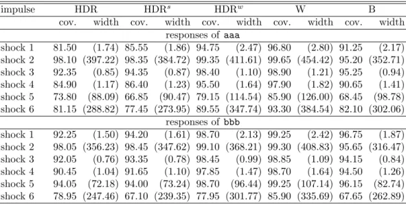
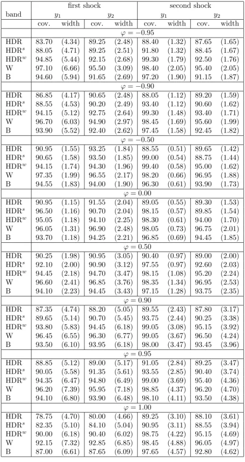
The results for DGP2 with estimated lag order, T = 200 and H = 12 are shown in Table 2, while Appendix D provides additional results on DGP2 for T = 200 and T = 400, horizons H = 12 and H = 24 and both assuming the true lag order and using the estimated lag order. All results for DGP2 refer only to the responses of the corporate bond spreads aaaand bbb, which are in the focus of the empirical application.

Results from Table 2 show that capturing uncertainty associated with response parameter estimates is more difficult in a larger and very persistent system. For T = 200 and H = 12 all the methods fail to achieve the target of 90% coverage for all the cases. The undercoverage is a function of the width of the bands and so, the largest deviations from the nominal level are observed for the narrowest bands (HDR and HDR^s) and the smallest deviations correspond to the widest Wald band. The HDR^w is larger in these settings than the Bonferroni region which allows to bring up the coverage rates of this band in the most problematic cases.

Table 2: Estimated coverage probabilities and mean widths (in parentheses) of 90% confidence bands for DGP2,T = 200,H = 12 and estimated lag order

impulse HDR HDR^s HDR^w W B

cov. width cov. width cov. width cov. width cov. width responses of aaa

shock 1 81.50 (1.74) 85.55 (1.86) 94.75 (2.47) 96.80 (2.80) 91.25 (2.17) shock 2 98.10 (397.22) 98.35 (384.72) 99.35 (411.61) 99.65 (454.42) 95.20 (352.71) shock 3 92.35 (0.85) 94.35 (0.87) 98.40 (1.10) 98.90 (1.21) 95.25 (0.94) shock 4 84.90 (1.17) 86.40 (1.23) 95.50 (1.64) 97.90 (1.82) 90.65 (1.41) shock 5 73.80 (88.09) 66.85 (90.47) 79.15 (114.54) 85.90 (126.00) 68.45 (98.78) shock 6 81.15 (288.82) 77.45 (273.95) 89.55 (347.74) 93.30 (384.54) 82.10 (302.06)

responses of bbb

shock 1 92.25 (1.50) 94.20 (1.61) 98.70 (2.13) 99.25 (2.42) 96.75 (1.87) shock 2 98.05 (356.23) 98.45 (347.62) 99.10 (368.21) 99.30 (408.83) 95.65 (316.47) shock 3 92.05 (0.76) 93.35 (0.78) 98.45 (0.99) 98.85 (1.09) 94.15 (0.84) shock 4 90.45 (1.04) 91.65 (1.10) 97.85 (1.47) 98.70 (1.64) 94.50 (1.26) shock 5 94.05 (72.18) 94.00 (73.24) 98.70 (96.44) 99.25 (107.14) 96.15 (82.74) shock 6 78.95 (247.46) 67.10 (239.35) 77.95 (301.77) 85.90 (335.69) 67.65 (262.89)

Conclusions from further results obtained for DGP2 and the case of un- known lag length (Tables 15–17 in Appendix D) are as follows: doubling the sample size, makes it possible to increase all the coverage rates above 80%.

Using the HDR, HDR^s and even B methods is still, however, associated with a risk of giving a false impression about the estimation precision. Another consequence of increasing the sample size is that the Wald bands become too wide as compared to the HDR^w bands. Increasing the horizon H to 24, works in favor of the Bonferroni band which can be considered competitive with the HDR^w band in this case.

There are no big changes in results under the more idealized condition of knowing the true order of the VAR (Tables 18–21 in the Appendix). Thus, the same conclusions as formulated for the lag length pestimated using AIC hold.

5 Application to Corporate Bond Spreads

The empirical example, which also served as blueprint for the more com- plex DGP2 in the Monte Carlo analysis, is based on a model proposed by Bundesbank (2005) and studied with regard to its forecasting performance by Staszewska-Bystrova and Winker (2014). In the context of analyzing the stability of the financial system, the model focused on determinants of cor- porate bond spreads, i.e., the gap between the returns on bonds considered as “safe” (German government bonds) and on more risky corporate bonds.

The model builds on a theoretical base discussed in detail in Bundesbank (2005, pp. 141ff). However, the reduced form VAR used for the empiri- cal analysis includes also some additional variables, which are considered as

potentially relevant. In particular, based on arguments from option price the- ory and macroeconomic portfolio theory, the model comprises a short-term money market rate as a monetary policy indicator and two corporate bond spreads corresponding to different levels of perceived risk. The growth rate of a stock market index reflects expectations concerning the business cycle and prices of assets as alternative to corporate bond spreads. Stock market volatility is used as proxy for uncertainty, which through its effect on firms’

value, i.e., distance-to-default, will affect corporate bond spreads. Finally, the interest rate curve is represented by the spread between 2- and 10-year government bonds.

The VAR model discussed in Bundesbank (2005, pp. 141ff) includes two additional endogenous variables, which are not considered in the present ap- plication due to problems with data availability and in order to limit the model dimension. The first variable is a measure of gross emissions of cor- porate bond spreads, which can be seen as a proxy for market liquidity, and the second variable relates outstanding loans to corporate profits.

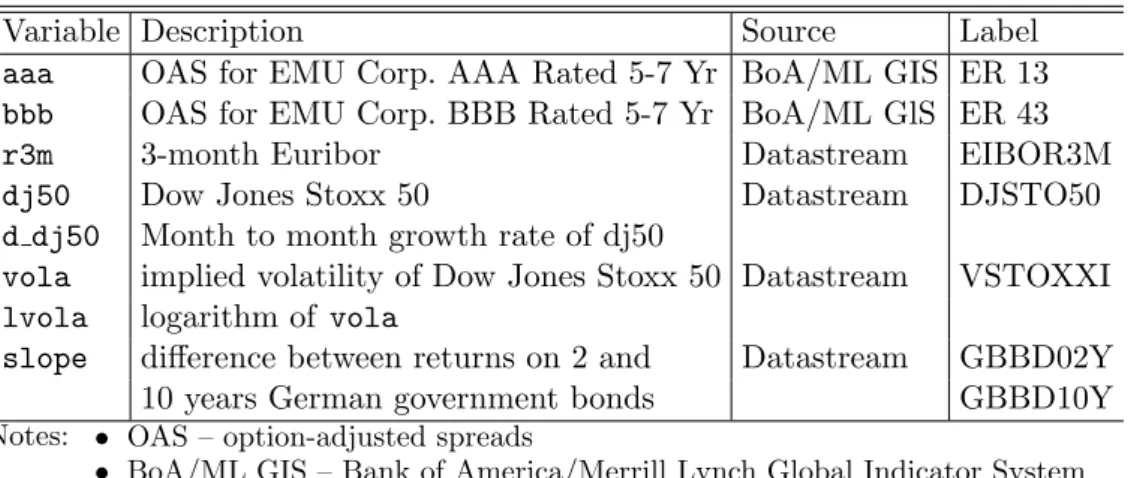
Apart from the omission of the two variables, our implementation follows the original VAR model as closely as possible, given available data. For the option adjusted spreads for Euro area corporate bonds with AAA and BBB rating, we choose a time to maturity of 5 to 7 years, instead of the 7 to 10 years in the original paper. This change is a consequence of limited availability of corporate bonds with time to maturity above 7 years after the financial market crisis which precludes the calculation of an index. Data are obtained from the Bank of America/Merrill Lynch global index system⁵ and denoted by aaa and bbb, respectively. Data for all other variables included in the VAR model are obtained from Datastream. The 3-month Euribor is chosen as short-term interest rate, which reflects both monetary policy and conditions on the interbank market. It is denoted as r3m. The monthly growth rate of the Dow Jones Stoxx 50, denoted as d dj50 is used as a stock market indicator. For stock market volatility representing a proxy for uncertainty, we use the logarithm of the implied volatility of the Dow Jones Stoxx 50, which is denoted by lvola. Finally, slope stands for the interest rate spread between 2- and 10-year government bonds. We decided to use the spread on German government bonds rather than the spread on all Euro denoted government bonds in order to exclude the effects of the sovereign debt crisis. Table 3 summarizes the data used for the VAR model.

The model includes six variables in the orderr3m, d dj50, lvola,slope, aaa, andbbb. This ordering corresponds to the one suggested in Bundesbank (2005, pp. 141ff). The model is estimated with monthly data for the sample starting with the introduction of the Euro in January 1999 and ending in June 2015. The sample size is T = 197, i.e., it is similar to the smaller sample size considered in the Monte Carlo simulations. Model selection based on the AIC with a maximum lag length of 8 months suggests a lag order of four. The estimation results for the 144 parameters describing the dynamics, the six constants and the 6×6 variance covariance matrix (rounded to four

5Seehttp://www.mlindex.ml.com/gispublic/default.asp.

Table 3: Labels, definition and source of series used for the VAR(4) model

Variable Description Source Label

aaa OAS for EMU Corp. AAA Rated 5-7 Yr BoA/ML GIS ER 13 bbb OAS for EMU Corp. BBB Rated 5-7 Yr BoA/ML GlS ER 43

r3m 3-month Euribor Datastream EIBOR3M

dj50 Dow Jones Stoxx 50 Datastream DJSTO50

d dj50 Month to month growth rate of dj50

vola implied volatility of Dow Jones Stoxx 50 Datastream VSTOXXI lvola logarithm of vola

slope difference between returns on 2 and Datastream GBBD02Y 10 years German government bonds GBBD10Y Notes: • OAS – option-adjusted spreads

• BoA/ML GIS – Bank of America/Merrill Lynch Global Indicator System

digits) are presented in Appendix A.

As for the Monte Carlo simulation, we consider impulse responses for horizons H = 12 and H = 24 corresponding to one and two years, respec- tively. Orthogonal impulse responses are calculated assuming the ordering of the variables mentioned earlier: r3m,d dj50,lvola,slope,aaa, and bbb.

This ordering ensures that change in the monetary policy instrument r3m can have a contemporaneous effect on all other variables in the system.

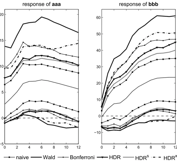
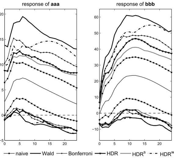
The impulse responses and corresponding joint confidence bands con- structed making use of the different methods presented in this study are shown in Figure 3 for H = 12 and in Figure 4 for H = 24, respectively. We also include the na¨ıve bands in the figures which are constructed by connect- ing pointwise 90% confidence intervals for each individual impulse response coefficient. It becomes apparent that while the overall shape of the confi- dence bands is similar for all methods considered, the widths of the bands differ substantially. The na¨ıve bands are the smallest but, as argued earlier, are likely to have a much smaller coverage probability than the desired 90%.

As might have been expected based on the simulation results presented in Table 2 in the previous section, the bands based on the Wald and on the HDR^w methods are the widest. Given that the smaller bands have a ten- dency for coverage rates below the desired nominal rate in the simulations, in particular with regard to the responses of aaa, considering Wald or HDR^w bands may be an appropriate choice. While none of the bands includes the zero line for all propagation horizons, significantly positive values are much more common for the narrower bands. The differences between the methods become even more pronounced, when the upper limit of the confidence bands is considered. In particular, the HDR^w band is smaller than the Wald band while maintaining an adequate coverage according to the simulation results.

Hence, it seems to be the best choice for the responses of aaa, assuming that the results from the simulation setting hold for the empirical model.

0 2 4 6 8 10 12

−5 0 5 10 15 20

response of aaa

0 2 4 6 8 10 12

−10 0 10 20 30 40 50 60

response of bbb

naive Wald Bonferroni HDR HDR^s HDR^w

Figure 3: 90% confidence bands for responses of aaaand bbbto a monetary policy shock for the empirical VAR(4) model, H = 12

0 5 10 15 20

−5 0 5 10 15 20

response of aaa

0 5 10 15 20

−10 0 10 20 30 40 50 60

response of bbb

naive Wald Bonferroni HDR HDR^s HDR^w

Figure 4: 90% confidence bands for responses of aaaand bbbto a monetary policy shock for the empirical VAR(4) model, H = 24

The qualitative findings concerning responses of bbb, differ even more markedly given that both the Wald and the HDR^w bands include zero for all periods up to H = 12 or H = 24, respectively. In these cases, one may conclude that there is no effect of the monetary policy shock on the corporate bond spread, while the narrower bands exclude zero for at least some of the propagation horizons. Given that all methods included in the Monte Carlo study are conservative for this IRF, one might consider resorting to the HDR or HDR^s bands in this case. However, for applied econometric work, the selection of different methods for constructing bands for a single model may not be convincing.

To sum up, for a specific empirical application based on a six-dimensional VAR model, joint confidence bands constructed with different approaches dif- fer not only quantitatively, but also with regard to the qualitative conclusions they imply. Based on the Monte Carlo simulation results, the HDR^w method appears to be a sensible choice when strong emphasis is placed on coverage properties of the bands. Substantially narrower HDR^s bands might carry the risk of underreporting the actual uncertainty.

6 Conclusion

In this study we have proposed and investigated the properties of non- parametric methods for constructing confidence bands for impulse responses based on the bootstrap and the highest density region approach. The den- sity estimation was applied to either unscaled bootstrapped response func- tions, responses scaled period-wise with the estimated standard deviations or whitened bootstrap replicates of the impulse responses.

The results of an extensive Monte Carlo study indicate that the HDR method is a promising tool for computing error bands for structural vector autoregressive analysis. In particular the method taking into account the correlation structure between the response parameter estimators (HDR^w) is superior to other methods in several dimensions. This method carries the smallest risk of underachieving the nominal coverage rate and is competitive with existing benchmarks, i.e. the Bonferroni and Wald approaches.

The advantages over the rather conservative Wald band can be seen for sample sizes exceeding very small ones and consist in reduced width and more precise coverage rates. As a result, the HDR^w bands are more informative than the Wald bands and hence are attractive for empirical applications. The dominance over the Bonferroni band is less pronounced, as the two types of bands are often quite similar. Nevertheless, the HDR^w method may have advantages, e.g., if the propagation horizon used in the analysis becomes large. This directly influences the width of the Bonferroni band which may easily become wider than the HDR^w band.

An empirical application using a six-dimensional VAR model shows that qualitative findings from impulse response analysis might change depending on the method used for constructing joint bands. Although no general con- clusions can be drawn from this example, the outcomes are in line with the

results from the Monte Carlo simulations.

Further research will address the robustness of the method under depar- tures from the underlying assumptions. Another extension is to investigate possible gains from increasing the number of bootstrap replications. This may improve the non-parametric point-wise approximation of a high dimen- sional distribution used in the HDR method.

Acknowledgements

Support from the National Science Center, Poland (NCN) through HARMO- NIA 6: UMO-2014/14/M/HS4/00901 and Deutsche Forschungsgemeinschaft through the SFB 649 “Economic Risk” are gratefully acknowledged. The research for this paper was conducted while the first author was Bundesbank Professor at the Freie Universit¨at Berlin. An earlier version of the paper was presented at the 9th International Conference on Computational and Finan- cial Econometrics, 2015 and at research seminars at Macquarie University, Sydney, the University of Sydney and the University of New South Wales in Sydney. Comments by the participants are gratefully acknowledged.

References

Bundesbank, Deutsche (2005). Finanzmarktstabilit¨atsbericht 2005. Deutsche Bundesbank. Frankfurt a.M.

Fresoli, D., E. Ruiz and L. Pascual (2015). Bootstrap multi-step fore- casts of non-Gaussian VAR models.International Journal of Forecasting 31(3), 834–848.

Hyndman, R.J. (1995). Highest-density forecast regions for nonlinear and non-normal time series models. Journal of Forecasting 14(5), 431–441.

Hyndman, R.J. (1996). Computing and graphing highest density regions.The American Statistician 50(2), 120–126.

Inoue, A. and L. Kilian (2016). Joint confidence sets for structural impulse responses. Journal of Econometrics p. forthcoming.

Jord`a, O. (2009). Simultaneous confidence regions for impulse responses.The Review of Economics and Statistics 91(3), 629–647.

Kilian, L. (1998). Small-sample confidence intervals for impulse response functions. Review of Economics and Statistics 80(2), 218–230.

Ledoit, O. and M. Wolf (2003). Improved estimation of the covariance matrix of stock returns with an application to portfolio selection. Journal of Empirical Finance 10(5), 603–621.

L¨utkepohl, H. (2005). New Introduction to Multiple Time Series Analysis.

Springer-Verlag. Berlin.

L¨utkepohl, H., A. Staszewska-Bystrova and P. Winker (2015a). Comparison of methods for constructing joint confidence bands for impulse response functions. International Journal of Forecasting 31(3), 782–798.

L¨utkepohl, H., A. Staszewska-Bystrova and P. Winker (2015b). Confidence bands for impulse responses: Bonferroni versus Wald. Oxford Bulletin of Economics and Statistics 77(6), 800–821.

Nicholls, D.F. and A.L. Pope (1988). Bias in estimation of multivariate au- toregression. Australian Journal of Statistics 30A(1), 296–309.

Sch¨afer, J. and K. Strimmer (2005). A shrinkage approach to large-scale covariance matrix estimation and implications for functional genomics.

Statistical Applications in Genetics and Molecular Biology 4(1), 1–32.

Scott, D.W. (1992). Multivariate Density Estimation: Theory, Practice, and Visualization. John Wiley & Sons. New York.

Staszewska-Bystrova (2013). Modified Scheff´e’s prediction bands.Jahrb¨ucher f¨ur National¨okonomie und Statistik 233(5–6), 680–690.

Staszewska-Bystrova, A. and P. Winker (2013). Constructing narrowest path- wise bootstrap prediction bands using threshold accepting.International Journal of Forecasting 29, 221–233.

Staszewska-Bystrova, A. and P. Winker (2014). Measuring forecats uncer- tainty of corporate bond spreads by Bonferroni-type prediction bands.

Central European Journal of Economic Modeling and Econometrics 6(2), 89–104.

Appendix

A DGP2 based on Corporate Bond Spreads

For the VAR model of corporate bond spreads discussed in Section 5, the variables are ordered as y = [r3m d dj50 lvola slope aaa bbb]⁰ both in the model and for the calculation of orthogonal impulse response functions.

From the estimation of a VAR(4) model (with intercepts) for the available data, the following (rounded) OLS parameter estimates result, which are used for the data based DGP used in Section 4. The modulus of the largest root of this DGP’s companion matrix is equal to 0.9846.

Ab₁ =

















1.4980 0.0001 0.2083 −0.0194 −0.0049 0.0005 85.0541 0.0946 95.8171 −58.6221 −2.4562 1.0396

−0.1518 −0.0000 0.6512 0.1253 0.0042 −0.0007

−0.1668 −0.0000 0.0592 0.9068 0.0081 −0.0019 11.7445 −0.0036 4.5559 1.7544 0.9544 −0.1109 26.3265 −0.0024 24.0634 20.9788 1.0234 0.8374

















Ab2 =

















−0.6398 −0.0001 −0.2583 −0.0684 0.0013 −0.0008

−78.7624 0.1046 48.5138 −17.5405 −0.1287 −0.7530 0.3310 0.0000 0.1092 −0.0513 −0.0036 0.0004 0.1296 0.0000 −0.0902 0.0216 −0.0073 0.0029

−2.4116 0.0033 −6.5170 1.6486 0.1795 0.1755

−32.4664 0.0002 −32.2479 −20.5660 −0.2242 −0.0399

















Ab₃ =

















0.3838 0.0001 0.1862 0.0147 0.0006 0.0004

−20.7017 0.1124 55.7656 135.3880 1.7755 −0.3592

−0.2284 −0.0001 0.0029 −0.1107 0.0007 −0.0005

−0.1356 −0.0004 −0.1141 0.0905 −0.0006 −0.0017

−4.9517 −0.0106 −1.9574 −7.1059 0.0485 −0.1459

−33.0704 −0.0262 −21.9510 −25.1256 0.3955 0.0591

















Ab4 =

















−0.2453 0.0000 −0.1124 0.0775 0.0024 −0.0002

−3.8015 −0.0351 −139.2140 −49.1099 −0.2717 0.2346 0.0620 0.0001 0.0601 0.0250 0.0004 0.0005 0.1620 0.0001 0.2075 −0.1063 0.0007 0.0005

−4.1185 −0.0027 1.4944 1.8785 −0.1641 0.0800 42.4863 −0.0000 17.7850 25.4542 −0.6164 −0.0021

















νb =

















−0.0120

−138.8264 0.5026

−0.0948 9.1030 29.9061

















Σbu =

















0.0000 0.0001 −0.0000 −0.0000 0.0000 −0.0000 0.0001 1.5924 −0.0013 −0.0001 −0.0398 −0.1265

−0.0000 −0.0013 0.0000 0.0000 0.0001 0.0002

−0.0000 −0.0001 0.0000 0.0000 0.0000 0.0001 0.0000 −0.0398 0.0001 0.0000 0.0110 0.0118

−0.0000 −0.1265 0.0002 0.0001 0.0118 0.0492

















×10⁴

B Further Results for DGP1 with Estimated

Lag Order