S F B
XXX
E C O N O M I C
R I S K
B E R L I N
SFB 649 Discussion Paper 2014-067
Bootstrap confidence sets under model
misspecification Vladimir Spokoiny*, **
Mayya Zhilova**
* Humboldt-Universität zu Berlin, Germany
** Weierstrass-Institute
This research was supported by the Deutsche
Forschungsgemeinschaft through the SFB 649 "Economic Risk".
http://sfb649.wiwi.hu-berlin.de ISSN 1860-5664
SFB 649, Humboldt-Universität zu Berlin Spandauer Straße 1, D-10178 Berlin
SFB
6 4 9
E C O N O M I C
R I S K
B E R L I N
Vladimir Spokoiny∗
Weierstrass-Institute, Humboldt University Berlin,
Moscow Institute of Physics and Technology, Mohrenstr. 39,
10117 Berlin, Germany, spokoiny@wias-berlin.de
Mayya Zhilova†
Weierstrass-Institute,
Mohrenstr. 39, 10117 Berlin, Germany, zhilova@wias-berlin.de November 17, 2014
Abstract
A multiplier bootstrap procedure for construction of likelihood-based confidence sets is considered for finite samples and a possible model misspecification. Theoretical results justify the bootstrap consistency for a small or moderate sample size and allow to control the impact of the parameter dimension p: the bootstrap approximation works if p3/n is small. The main result about bootstrap consistency continues to apply even if the underlying parametric model is misspecified under the so called Small Modeling Bias condition. In the case when the true model deviates significantly from the considered parametric family, the bootstrap procedure is still applicable but it becomes a bit conservative:
the size of the constructed confidence sets is increased by the modeling bias. We illustrate the results with numerical examples for misspecified constant and logistic regressions.
JEL classification codes: C13, C15
Keywords: likelihood-based bootstrap confidence set, misspecified model, finite sample size, multiplier bootstrap, weighted bootstrap, Gaussian approximation, Pinsker’s in- equality
∗The author is partially supported by Laboratory for Structural Methods of Data Analysis in Pre- dictive Modeling, MIPT, RF government grant, ag. 11.G34.31.0073. Financial support by the German Research Foundation (DFG) through the Research Unit 1735 is gratefully acknowledged
†Financial support by the German Research Foundation (DFG) through the Collaborative Research Center 649 “Economic Risk” is gratefully acknowledged
1
1 Introduction
Since introducing in 1979 by Efron (1979) the bootstrap procedure became one of the most powerful and common tools in statistical confidence estimation and hypothesis test- ing. Many versions and extensions of the original bootstrap method have been proposed in the literature; see e.g. Wu (1986); Newton and Raftery (1994); Barbe and Bertail (1995);Horowitz(2001);Chatterjee and Bose(2005);Ma and Kosorok(2005);Chen and Pouzo (2009); Lavergne and Patilea (2013); Chen and Pouzo (2014) among many oth- ers. This paper focuses on the multiplier bootstrap procedure which attracted a lot of attention last time due to its nice theoretical properties and numerical performance. We mention the papers Chatterjee and Bose (2005), Arlot et al. (2010) and Chernozhukov et al. (2013) for the most advanced recent results. Chatterjee and Bose (2005) showed some results on asymptotic bootstrap consistency in a very general framework: for esti- mators obtained by solving estimating equations. Chernozhukov et al.(2013) presented a number of non-asymptotic results on bootstrap validity with applications to special problems like testing many moment restrictions or parameter choice for a LASSO proce- dure. Arlot et al. (2010) constructed a non-asymptotical confidence bound in `s norm (s ∈ [1,∞] ) for the mean of a sample of high dimensional i.i.d. Gaussian vectors (or with a symmetric and bounded distribution), using the generalized weighted bootstrap for resampling of the quantiles.
This paper makes a further step in studying the multiplier bootstrap method in the problem of confidence estimation by a quasi maximum likelihood method. For a rather general parametric model, we consider likelihood-based confidence sets with the radius determined by a multiplier bootstrap. The aim of the study is to check the validity of the bootstrap procedure in situations with a large parameter dimension, a limited sample size, and a possible misspecification of the parametric assumption. The main result of the paper explicitly describes the error term of the bootstrap approximation.
This particularly allows to track the impact of the parameter dimension p and of the sample size n in the quality of the bootstrap procedure. As one of the corollaries, we show bootstrap validity under the constraint “p3/n-small”. Chatterjee and Bose (2005) stated results under the condition “p/n-small” but their results only apply to low dimensional projections of the MLE vector. In the likelihood based approach, the construction involves the Euclidean norm of the MLE which leads to completely different tools and results. Chernozhukov et al.(2013) allowed a huge parameter dimension with
“ log(p)/n small” but they essentially work with a family of univariate tests which again differs essentially from the maximum likelihood approach.
Another interesting and important issue is the impact of the model misspecification
on the accuracy of bootstrap approximation. A surprising corollary of our error bounds is that the bootstrap confidence set can be used even if the underlying parametric model is slightly misspecified under the so calledsmall modeling bias (SmB) condition. If the modeling bias becomes large, the bootstrap confidence sets are still applicable, but they become more and more conservative. (SmB) condition is given in Section 4 and it is consistent with classical bias-variance relation in nonparametric estimation.
Our theoretical study uses the square-root Wilks (sq-Wilks) expansion fromSpokoiny (2012a), Spokoiny (2013) which approximates the square root likelihood ratio statistic by the norm of the standardized score vector. Further we extend the sq-Wilks expansion to the bootstrap log-likelihood and adopt the Gaussian approximation theory (GAR) to the special case when the distribution of the Euclidean norm of a non-Gaussian vector is approximated by the distribution of the norm of a Gaussian one with the same first and second moments. The Gaussian comparison technique based on the Pinsker inequality completes the study and allows to bridge the real unknown coverage probability and the conditional bootstrap coverage probability under (SmB) condition. In the case of a large modeling bias we state a one-sided bound: the bootstrap quantiles are uniformly larger than the real ones. This effect is nicely confirmed by our simulation study.
Now consider the problem and the approach in more detail. Let the data sample Y = (Y1, . . . , Yn)> consist ofindependent random observations and belong to the probability space (Ω,F, IP) . We do not assume that the observations Yi are identically distributed, moreover, no specific parametric structure of IP is being required. In order to explain the idea of the approach we start here with a parametric case, however the assumption (1.1) below is not required for the results. Let IP belong to some known regular parametric family {IPθ} def= {IPθ µ0,θ∈Θ⊂IRp}. In this case the true parameter θ∗ ∈ Θ is such that
IP ≡IPθ∗∈ {IPθ}, (1.1) and the initial problem of finding the properties of unknown distribution IP is reduced to the equivalent problem for the finite-dimensional parameter θ∗. The parametric family
{IPθ} induces the log-likelihood process L(θ) of the sample Y : L(θ) =L(Y,θ)def= log
dIPθ dµ0
(Y)
and the maximum likelihood estimate (MLE) of θ∗:
eθdef= argmaxθ∈ΘL(θ). (1.2)
The asymptotic Wilks phenomenonWilks(1938) states that for the case of i.i.d. obser- vations with the sample size tending to the infinity the likelihood ratio statistic converges
in distribution to χ2p/2 , where p is the parameter dimension:
2
L(eθ)−L(θ∗) −→w χ2p, n→ ∞.
Define the likelihood-based confidence set as E(z)def=
n
θ :L(eθ)−L(θ)≤z2/2 o
, (1.3)
then the Wilks phenomenon implies IPn
θ∗ ∈E(zα, χ2
p)o
→α, n→ ∞, where z2α, χ2
p is the (1−α) -quantile for the χ2p distribution. This result is very important and useful under the parametric assumption, i.e. when (1.1) holds. In this case the limit distribution of the likelihood ratio is independent of the model parameters or in other words it ispivotal. By this result a sufficiently large sample size allows to construct the confidence sets for θ∗ with a given coverage probability. However, a possibly low speed of convergence of the likelihood ratio statistic makes the asymptotic Wilks result hardly applicable to the case of small or moderate samples. Moreover, the asymptotical pivotal- ity breaks down if the parametric assumption (1.1) does not hold (see Huber (1967)), and, therefore, the whole approach may be misleading if the model is considerably mis- specified. If the assumption (1.1) does not hold, then the “true” parameter is defined by the projection of the true measure IP on the parametric family {IPθ}:
θ∗def= argmaxθ∈ΘIEL(θ). (1.4)
The recent results bySpokoiny (2012a), Spokoiny(2013) provide a non-asymptotic ver- sion of square-root Wilks phenomenon for the case of misspecified model. It holds with an exponentially high probability
q 2
L(eθ)−L(θ∗) − kξk
≤∆W' p
√n, (1.5)
where ξ def= D0−1∇θL(θ∗) , D02 def= −∇2θIEL(θ∗) . The bound is non-asymptotical, the approximation error term ∆W has an explicit form (the precise statement is given in TheoremA.2, Section A.1, and it depends on the parameter dimension p, sample size n, and the probability of the random set on which the result holds.
Due to this bound, the original problem of finding a quantile of the LR test statistic L(eθ) −L(θ∗) is reduced to a similar question for the approximating quantity kξk. The difficulty here is that in general kξk is non-pivotal, it depends on the unknown distribution IP and the target parameter θ∗. Another result bySpokoiny(2012b) gives
the following non-asymptotical deviation bound for kξk2: for some explicit constant C >0 it holds for x≥√
p
IP kξk2≥IEkξk2+Cx
≤ 2e−x
(the precise statement is given in Theorem A.3. This is a non-asymptotic deviation bound, sharp in leading approximating terms, however, the critical values yielded by it are too conservative for a valuable confidence set.
In the present work we study the multiplier bootstrap (or weighted bootstrap) pro- cedure for estimation of the quantiles of the likelihood ratio statistic. The idea of the procedure is to mimic a distribution of the likelihood ratio statistic by reweighing its summands with random multipliers independent of the data:
Lab(θ) def= Xn i=1log
dIPθ dµ0(Yi)
ui.
Here the probability distribution is taken conditionally on the data Y , which is denoted by the sign ab. The random weights u1, . . . , un are i.i.d. with continuos c.d.f., indepen- dent of Y and it holds for them: IE(ui) = 1 , Var(ui) = 1 , IEexp(ui)<∞. Therefore, the multiplier bootstrap induces the probability space conditional on the data Y . A simple but important observation is that IEabLab(θ)≡IE
Lab(θ) Y
=L(θ) , and hence,
argmaxθIEabLab(θ) = argmaxθL(θ) =θ.e
This means that the target parameter in the bootstrap world is precisely known and it coincides with the maximum likelihood estimator θe conditioned on Y , therefore, the bootstrap likelihood ratio statistic Lab(eθab)−Lab(eθ) def= supθ∈ΘLab(θ)−Lab(eθ) is fully computable and leads to a simple computational procedure for the approximation of the distribution of L(eθ)−L(θ∗) .
The goal of the present study is to show in a non-asymptotic way the consistency of the described multiplier bootstrap procedure and to obtain an explicit bound on the error of coverage probability. In other words, we are interested in non-asymptotic approximation of the distribution of
L(eθ)−L(θ∗) 1/2 with the distribution of
Lab(eθab)−Lab(eθ) 1/2. So far there exist very few theoretical non-asymptotic results about bootstrap validity.
Important contributions are given in the works byChernozhukov et al. (2013) andArlot et al.(2010). Finite sample methods for study of the bootstrap validity are essentially dif- ferent from the asymptotic ones which are mainly based on weak convergence arguments.
The main steps of our theoretical study are illustrated by the following scheme:
sq-Wilks theorem
Gauss.
approx.
Y-world:
q
2L(eθ)−2L(θ∗) ≈ kξk ≈w kξk
≈ w Gauss.compar. (1.6)
Bootstrap world:
q
2Lab(eθab)−2Lab(eθ) ≈ kξabk ≈w kξabk, where ξab def= D0−1∇θ
Lab(θ∗)−IE
Lab(θ∗)
Y ; compare with the definition (1.5) of the vector ξ in the Y -world. The vectors ξ and ξab are zero mean Gaussian and they mimic the covariance structure of the vectors ξ and ξab: ξ ∼N(0,Varξ) , ξab ∼ N 0,Var{ξab
Y} .
The upper line of the scheme corresponds to the Y -world, the lower line - to the bootstrap world. In both lines we apply two steps for approximating the corresponding likelihood ratio statistics. The first approximating step is the non-asymptotic square-root Wilks theorem: the bound (1.5) for the Y case and a similar statement for the bootstrap case, which is obtained in TheoremA.4, Section A.2.
The next step is called Gaussian approximation (GAR) which means that the dis- tribution of the Euclidean norm kξk of a centered random vector ξ is close to the distribution of the similar norm of a Gaussian vector kξk with the same covariance ma- trix as ξ. A similar statement holds for the vector ξab. Thus, the initial problem of comparing the distributions of the likelihood ratio statistics is reduced to the comparison of the distributions of the Euclidean norms of two centered normal vectors ξ and ξab (Gaussian comparison). This last step links their distributions and encloses the approx- imating scheme. The Gaussian comparison step is done by computing the Kullback- Leibler divergence between two multivariate Gaussian distributions (i.e. by comparison of the covariance matrices of ∇θL(θ∗) and ∇θLab(θ∗) ) and applying Pinsker’s inequality (Lemma 5.7). At this point we need to introduce the “small modeling bias” condition (SmB) from Section4.2. It is formulated in terms of the following nonnegative-definite p×p symmetric matrices:
H02 def= Xn i=1IEh
∇θ`i(θ∗)∇θ`i(θ∗)>i
, (1.7)
B02 def= Xn
i=1IE[∇θ`i(θ∗)]IE[∇θ`i(θ∗)]>, (1.8) so that Var{∇θL(θ∗)} = H02 −B02. If the parametric assumption (1.1) is true or if the data Y are i.i.d., then it holds IE[∇θ`i(θ∗)] ≡ 0 and B02 = 0 . The (SmB) condition roughly means that the bias term B20 is small relative to H02. Below we show that the Kullback-Leibler distance between the distributions of two Gaussian vectors
ξ and ξab is bounded by pkH0−1B02H0−1k2/2 . The (SmB) condition precisely means that this quantity is small. We consider two situations: when the condition (SmB) is fulfilled and when it is not. Theorem 2.1 in Section 2 deals with the first case, it provides the cumulative error term for the coverage probability of the confidence set (1.3), taken at the (1−α) -quantile computed with the multiplier bootstrap procedure.
The proof of this result (see Section A.3) summarizes the steps of scheme (1.6). The biggest term in the full error is induced by Gaussian approximation and requires the ratio p3/n to be small. In the case of a “large modelling bias” i.e., when (SmB) does not hold, the multiplier bootstrap procedure continues to apply. It turns out that the bootstrap quantile increases with the growing modelling bias, hence, the confidence set based on it remains valid, however, it may become conservative. This result is given in Theorem2.4 of Section2. The problems of Gaussian approximation and comparison for the Euclidean norm are considered in Sections5.2and5.4in general terms independently of the statistical setting of the paper, and might be interesting by themselves. Section 5.4presents also an anti-concentration inequality for the Euclidean norm of a Gaussian vector. This inequality shows how the deviation probability changes with a threshold.
The general results on GAR are summarized in Theorem5.1and restated in Proposition A.9for the setting of scheme (1.6). These results are also non-asymptotic with explicit errors and apply under the condition that the ratio p3/n to be small.
In Theorem 2.3 we consider the case of a scalar parameter p= 1 with an improved error term. Furthermore in Section 2.1 we propose a modified version of a quantile function based on a smoothed probability distribution. In this case the obtained error term is also better, than in the general result.
Notations: k · k denotes Euclidean norm for vectors and spectral norm for matrices;
C is a generic constant. The value x > 0 describes our tolerance level: all the results will be valid on a random set of probability ( 1−Ce−x) for an explicit constant C. Everywhere we give explicit error bounds and show how they depend on p and n for the case of the i.i.d. observations Y1, . . . , Yn and x ≤ Clogn. More details on it are given in Section4.3.
The paper is organized as follows: the main results are stated in Section 2, their proofs are given in Sections A.3, A.4 and A.5; Section 3 contains numerical results for misspecified constant and logistic regressions. In Section 4 we give all the necessary conditions and provide an information about dependency of the involved terms on n and p. Section 5 collects some useful statements on Gaussian approximation and Gaussian comparison.
2 Multiplier bootstrap procedure
Let `i(θ) denote the parametric log-density of the i-th observation:
`i(θ)def= log dIPθ
dµ0
(Yi)
, then L(θ) = Pn
i=1`i(θ). Consider i.i.d. scalar random variables ui independent of Y with continuous c.d.f., IEui = 1 , Varui = 1 , IEexp(ui) < ∞ for all i = 1, . . . , n. Multiply the summands of the likelihood function L(θ) with the new random variables:
Lab(θ)def= Xn
i=1`i(θ)ui,
then it holds IEabLab(θ) =L(θ) , where IEab stands for the conditional expectation given Y :
IEab(·)def= IE(·|Y), IP ab(·)def= IP(·|Y).
Therefore, the quasi MLE for the Y -world is a target parameter for the bootstrap world:
argmaxθ∈ΘIEabLab(θ) = argmaxθ∈ΘL(θ) =θ.e
The corresponding quasi MLE under the conditional measure IP ab is defined θeabdef= argmaxθ∈ΘLab(θ).
The likelihood ratio statistic in the bootstrap world is equal to Lab(eθab)−Lab(eθ) , where all the elements: the function Lab(θ) and the arguments eθab, eθ are known and available for computation.
Let 1−α∈(0,1) be a fixed desirable confidence level of the set E(z) :
IP(θ∗ ∈E(z)) ≥1−α. (2.1)
Here the parameter z ≥ 0 determines the size of the confidence set. Usually we are interested in finding a set of the smallest possible diameter satisfying this property. This leads to the problem of fixing the minimal possible value of z such that (2.1) is fulfilled.
Let zα denote the upper α-quantile of the square-root likelihood ratio statistic:
zαdef= min n
z≥0 :IP
L(θ)e −L(θ∗)>z2/2
≤α o
. (2.2)
This means, that zα is exactly the value of our interest. Estimation of zα leads to recov- ering of the distribution of L(eθ)−L(θ∗) . The multiplier bootstrap procedure consists of generating a large number of independent samples {u1, . . . , un} and computing from
them the empirical distribution function of Lab(eθab)−Lab(eθ) . By this procedure we can estimate zαab, the upper α-quantile of
q
2Lab(eθab)−2Lab(eθ) : zαab def= min
n
z≥0 :IP ab
Lab(eθab)−Lab(eθ)>z2/2
=α o
. (2.3)
Theorem 2.1(Validity of the bootstrap under a small modeling bias). Let the conditions of Section 4 be fulfilled. It holds with probability ≥ 1−12e−x for zαab ≥ max{2,√
p}+ C(p+x)/√
n:
IP
L(θ)e −L(θ∗)>(zαab)2/2
−α
≤ ∆full, (2.4)
where ∆full ≤C{(p+x)3/n}1/8 in the case 4.3. An explicit definition of the error term
∆full is given in the proof (see (A.26), (A.27) in SectionA.3).
The term ∆full can be viewed as a sum of the error terms corresponding to each step in the scheme (1.6). The largest error term equal to C{(p+x)3/n}1/8 is induced by GAR.
This error rate is not always optimal for GAR, e.g. in the case of p= 1 or for the i.i.d.
observations (see Remark5.2). In Theorems 2.3and 2.5the rate is C{(p+x)3/n}1/2. In view of definition (1.3) of the likelihood-based confidence set Theorem 2.1implies the following
Corollary 2.2 (Coverage probability error). Under the conditions of Theorem 2.1 it holds:
|IP{θ∗ ∈E(zαab)} −(1−α)| ≤ ∆full.
Remark 2.1 (Critical dimension). The error term ∆full depends on the ratio p3/n. The bootstrap validity can be only stated if this ratio is small. The obtained error bound seems to be mainly of theoretical interest, because the condition “ (p3/n)1/8 is small”
may require a huge sample. However, it provides some qualitative information about the bootstrap behavior as the parameter dimension grows. Our numerical results show that the accuracy of bootstrap approximation is very reasonable in a variety of examples.
In the following theorem we consider the case of a scalar parameter p = 1 . The obtained error rate is 1/√
n, which is sharper, than 1/n1/8. Instead of the GAR for the Euclidean norm from Section5we use here Berry-Esseen theorem (see also Remark5.2).
Theorem 2.3 (The case of p= 1 , using Berry-Esseen theorem). Let the conditions of Section 4 be fulfilled. It holds with probability ≥1−12e−x for zαab ≥1 +C(1 +x)/√
n:
IP
L(θ)e −L(θ∗)>(zαab)2/2
−α
≤ ∆B.E.,full, (2.5)
where ∆B.E.,full ≤ C(1 +x)/√
n in the case 4.3. An explicit definition of ∆B.E.,full is given in(A.28) in SectionA.3.
Remark 2.2 (Bootstrap validity and weak convergence). The standard way of proving the bootstrap validity is based on weak convergence arguments; see e.g. Mammen(1992), van ver Vaart and Wellner(1996),Janssen and Pauls(2003),Chatterjee and Bose(2005).
If the statistic L(eθ)−L(θ∗) weakly converges to a χ2-type distribution, one can state an asymptotic version of the results (2.4), (2.5). Our way is based on a kind of non- asymptotic Gaussian approximation and Gaussian comparison for random vectors and allows to get explicit error terms.
Remark 2.3 (Use of Edgeworth expansion). The classical results on confidence sets for the mean of population states the accuracy of order 1/n based on the second order Edgeworth expansionHall(1992). Unfortunately, if the considered parametric model can be misspecified, even the leading term is affected by the modeling bias, and the use of Edgeworth expansion cannot help in improving the bootstrap accuracy.
Remark 2.4 (Choice of the weights). In our construction, similarly to Chatterjee and Bose (2005), we apply a general distribution of the bootstrap weights ui under some moment conditions. One particularly can use Gaussian multipliers as suggested byCher- nozhukov et al.(2013). This leads to the exact Gaussian distribution of the vectors ξab and is helpful to avoid one step of Gaussian approximation for these vectors.
Now we discuss the impact of modeling bias, which comes from a possible misspeci- fication of the parametric model. As explained by the approximating diagram (1.6), the distance between the distributions of the likelihood ratio statistics can be characterized via the distance between two multivariate normal distributions. To state the result let us recall the definition of the full Fisher information matrix D20 def= −∇2θIEL(θ∗) . For the matrices H02 and B20, given in (1.7) and (1.8), it holds H02 > B02 ≥0 . If the parametric assumption (1.1) is true or in the case of an i.i.d. sample Y , B02 = 0 . Under the condition (SmB) kH0−1B02H0−1k enters linearly in the error term ∆full in Theorem2.1.
The first statement in Theorem2.4below says that the effective coverage probability of the confidence set based on the multiplier bootstrap islargerthan the nominal coverage probability up to the error term ∆b,full≤C{(p+x)3/n}1/8. The inequalities in the second part of Theorem2.4 prove the conservativeness of the bootstrap quantiles: the quantity q
tr{D0−1H02D0−1} − q
tr{D0−1(H02−B20)D0−1} ≥0 increases with the growing modeling bias.
Theorem 2.4 (Performance of the bootstrap for a large modeling bias). Under the conditions of Section 4 except for (SmB) it holds with probability ≥ 1 −14e−x for
z,zαab ≥max{2,√
p}+C(p+x)/√ n 1. IP
L(eθ)−L(θ∗)>z2/2
≤IPab
Lab(θeab)−Lab(θ)e >z2/2
+∆b,full.
2. zαab ≥z(α+∆
b,full)
+ q
tr{D0−1H02D0−1} − q
tr{D−10 (H02−B02)D−10 } −∆qf,1, zαab ≤z(α−∆
b,full)
+ q
tr{D0−1H02D0−1} − q
tr{D−10 (H02−B02)D−10 }+∆qf,2.
The term ∆b,full ≤ C{(p+x)3/n}1/8 is given in (A.30) in Section A.4. The positive values ∆qf,1, ∆qf,2 are given in (A.34), (A.33) in Section A.4, they are bounded from above with (a2 +a2B)(√
8xp+ 6x) for the constants a2,a2B > 0 from conditions (I), (IB).
Remark 2.5. There exists some literature on robust (and heteroscedasticity robust) bootstrap procedures; see e.g. Mammen (1993), Aerts and Claeskens(2001),Kline and Santos(2012). However, up to our knowledge there are no robust bootstrap procedures for the likelihood ratio statistic, most of the results compare the distribution of the estimator obtained from estimating equations, or Wald / score test statistics with their bootstrap counterparts in the i.i.d. setup. In our context this would correspond to the noise misspecification in the log-likelihood function and it is addressed automatically by the multiplier bootstrap. Our notion of modeling bias includes the situation when the target value θ∗ from (1.4) only defines a projection (the best parametric fit) of the data distribution. In particularly, the quantities IE∇θ`i(θ∗) for different i do not necessarily vanish yielding a significant modeling bias. Similar notion of misspecification is used in the literature on Generalized Method of Moments; see e.g. Hall (2005). Chapter 5 therein considers the hypothesis testing problem with two kinds of misspecification: local and non-local, which would correspond to our small and large modeling bias cases.
An interesting message of Theorem 2.4 is that the multiplier bootstrap procedure ensures a prescribed coverage level for this target value θ∗ even without small modeling bias restriction, however, in this case the method is somehow conservative because the modeling bias is transferred into the additional variance in the bootstrap world. The numerical experiments in Section3 agree with this result.
2.1 Smoothed version of a quantile function
This section briefly discusses the use of a smoothed quantile function. The (1−α) - quantile of
q
2L(eθ)−2L(θ∗) is defined as zα def= minn
z≥0 :IP
L(eθ)−L(θ∗)>z2/2
≤αo
= minn
z≥0 :IE1In
L(eθ)−L(θ∗)>z2/2o
≤αo .
Introduce for x≥0 and z, ∆ >0 the following function g∆(x, z)def= g
1
2∆z x2−z2
, (2.6)
where g(·) ∈ C2(IR) is a non-negative function, which grows monotonously from 0 to 1 , g(x) = 0 for x≤0 and g(x) = 1 for x≥1 , therefore:
1I{x≥1} ≤g(x)≤1I{x≥0} ≤g(x+ 1).
An example of such function is given in (5.9). In (5.10) it is shown 1I{x−z≥∆} ≤g∆(x, z)≤1I(x−z≥0)≤g∆(x, z+∆).
This approximation is used in the proofs of Theorems2.1and2.4in the part of Gaussian approximation of Euclidean norm of a sum of independent vectors (see Section 5.2) yielding the error rate (p3/n)1/8 in the final bound (Theorems2.1,5.1). The next result shows that the use of a smoothed quantile function helps to improve the accuracy of bootstrap approximation: it becomes (p3/n)1/2 instead of (p3/n)1/8. The reason is that we do not need to account for the error induced by a smooth approximation of the indicator function.
Theorem 2.5(Validity of the bootstrap in the smoothed case under (SmB) condition).
Let the conditions of Section 4 be fulfilled. It holds with probability ≥ 1−12e−x for z≥max{2,√
p}+C(p+x)/√
n and ∆∈(0,0.22]:
IEg∆ q
2L(eθ)−2L(θ∗),z
−IEabg∆ q
2Lab(eθab)−2Lab(eθ),z
≤∆sm,
where ∆sm ≤ C{(p+x)3/n}1/2∆−3 in the case 4.3. An explicit definition of ∆sm is given in(A.38), (A.39) in SectionA.5.
The modified bootstrap quantile function reads as z∆, αab def= min
z≥0 :IEabg∆
q
2Lab(eθab)−2Lab(eθ),z
=α
.
3 Numerical results
This section illustrates the performance of the multiplier bootstrap for some artificial examples. We especially aim to address the issues of noise misspecification and of in- creasing modeling bias. In all the experiments we took 104 data samples for estimation
of empirical c.d.f. of q
2L(eθ)−2L(θ∗) , 104 {u1, . . . , un} samples and 104 data samples for the estimation of the quantiles of
q
2Lab(θeab)−2Lab(θ) . All sample sizes aree n= 50 . It should be mentioned that the obtained results are nicely consistent with the theoretical statements.
3.1 Computational error
Here we check numerically, how well the multiplier procedure works in the case of the correct model. Let the i.i.d. data follow the distribution Yi∼N(2,1) , i= 1, . . . , n. The true likelihood function is L(θ) =−Pn
i=1(Yi−θ)2/2.
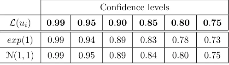
Table1shows the effective coverage probabilities of the quantiles estimated using the multiplier bootstrap. The second line contains the range of the nominal confidence levels:
0.99, . . . ,0.75 . The first left column describes the distribution of the bootstrap weights:
N(1,1) or exp(1) . The 3-d and the 4-th lines show the frequency of the event: “the real likelihood ratio ≤ the quantile of the bootstrap likelihood ratio”.
Table 1: Coverage probabilities for the correct i.i.d. model Confidence levels
L(ui) 0.99 0.95 0.90 0.85 0.80 0.75 exp(1) 0.99 0.94 0.89 0.83 0.78 0.73 N(1,1) 0.99 0.95 0.89 0.84 0.80 0.75
3.2 Constant regression with misspecified heteroscedastic errors
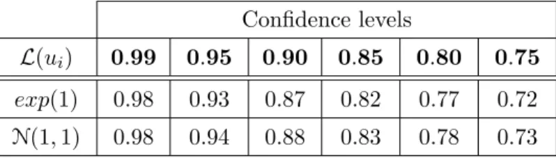
Here we show on a constant regression model that the quality of the confidence sets obtained by the multiplier bootstrap procedure is not significantly deteriorated by mis- specified heteroscedastic errors. Let the data be defined as Yi = 2 +σiεi, i= 1, . . . , n. The i.i.d. random variables εi ∼ Lap(0,2−1/2) are s.t. IE(εi) = 0 , Var(εi) = 1 . The coefficients σi are deterministic: σi
def= 0.5{4−i (mod 4)}. The quasi-likelihood func- tion is the same as in the previous experiment: L(θ) = −Pn
i=1(Yi −θ)2/2 , i.e. it is misspecified, since it corresponds to the i.i.d. standard normal distribution. Table 2 describes the 2 -nd experiment’s results similarly to the Table1.
Table 2: Coverage probabilities for the misspecified heteroscedastic noise Confidence levels
L(ui) 0.99 0.95 0.90 0.85 0.80 0.75 exp(1) 0.98 0.93 0.87 0.82 0.77 0.72 N(1,1) 0.98 0.94 0.88 0.83 0.78 0.73
3.3 Biased constant regression with misspecified errors
In the third experiment we consider biased regression with misspecified i.i.d. errors:
Yi =βsin(Xi) +εi, εi ∼Lap(0,2−1/2), i.i.d, Xi are equidistant in [0,2π].
Taking the likelihood function L(θ) = −Pn
i=1(Yi−θ)2/2 yields θ∗ = 0 . Therefore, the larger is the deterministic amplitude β >0 , the bigger is bias of the mean constant regression. We consider two cases: β = 0.25 with fulfilled (SmB) condition and β = 1.25 when (SmB) does not hold. Table 3 shows that for the large bias quantiles yielded by the multiplier bootstrap are conservative. This conservative property of the
Table 3: Coverage probabilities for the misspecified biased regression Confidence levels
L(ui) β 0.99 0.95 0.90 0.85 0.80 0.75 N(1,1) 0.25 0.98 0.94 0.89 0.84 0.79 0.74 1.25 1.0 0.99 0.97 0.94 0.91 0.87
multiplier bootstrap quantiles is also illustrated with the graphs in Figure 3.1. They show the empirical distribution functions of the likelihood ratio statistics L(θ)e −L(θ∗) and Lab(eθab)−Lab(eθ) for β = 0.25 and β = 1.25 . On the right graph for β = 1.25 the empirical distribution functions for the bootstrap case are smaller than the one for the Y case. It means that for the large bias the bootstrap quantiles are bigger than the Y quantiles, which increases the diameter of the confidence set based on the bootstrap quantiles. This confidence set remains valid, since it still contains the true parameter with a given confidence level.
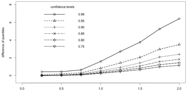
Figure3.2shows the growth of the difference between the quantiles of Lab(eθab)−Lab(eθ) and L(θ)−L(θe ∗) with increasing β for the range of the confidence levels: 0.75,0.8, . . . ,0.99 .
Figure 3.1: Empirical distribution functions of the likelihood ratios
Yi = 0.25 sin(Xi) +Lap(0,2−1/2), n= 50 Yi = 1.25 sin(Xi) +Lap(0,2−1/2), n= 50 empirical distribution function of L(θ)e −L(θ∗) estimated with 104 Y samples 50 empirical distribution functions of Lab(eθab)−Lab(eθ) estimated with 104 {ui} ∼exp(1) samples
Figure 3.2: The difference “Bootstrap quantile”−“Y -quantile”
growing with mod- eling bias
3.4 Logistic regression with bias
In this example we consider logistic regression. Let the data come from the following distribution:
Yi∼Bernoulli(βXi), Xi are equidistant in [0,2], β ∈(0,1/2].
Consider the likelihood function corresponding to the i.i.d. observations:
L(θ) =Xn i=1
n
Yiθ−log(1 + eθ) o
.
By definition (1.4) θ∗ = log{β/(1−β)}, bigger values of β induce larger modeling bias. The graphs below demonstrate the conservativeness of bootstrap quantiles. Here we consider two cases: β = 0.1 and β = 0.5 . Similarly to the Example 3.3 in the case of the bigger β on the right graph in Figure 3.3 the empirical distribution functions of Lab(θeab)−Lab(θ) are smaller than the one fore L(θ)e −L(θ∗) .
Figure 3.3:
Yi ∼Bernoulli(0.1Xi), n= 50 Yi∼Bernoulli(0.5Xi), n= 50
empirical distribution function of L(eθ)−L(θ∗) estimated with 104 Y samples 50 empirical distribution functions of Lab(θeab)−Lab(θ) estimated with 10e 4 {ui} ∼exp(1) samples
4 Conditions
Here we state the conditions necessary for the main results. The conditions in Section 4.1 come from the general finite sample theory by Spokoiny (2012a), they are required
for the results of Sections A.1 and A.2. Spokoiny (2012a) considers the examples of i.i.d. setup, generalized linear model and linear median regression providing a check of conditions from Section 4.1. The conditions in Section 4.2 are necessary to prove the results on multiplier bootstrap from Section2.
4.1 Basic conditions
Introduce the stochastic part of the likelihood process: ζ(θ) def= L(θ)−IEL(θ) , and its marginal summand: ζi(θ)def= `i(θ)−IE`i(θ) .
(ED0) There exist a positive-definite symmetric matrix V02 and constants g>0, ν0 ≥1 such that Var{∇θζ(θ∗)} ≤V02 and
sup
γ∈IRp
logIEexp
λγ>∇θζ(θ∗) kV0γk
≤ν02λ2/2, |λ| ≤g.
(ED2) There exists a constant ω ≥0 and for each r>0 a constant g2(r) such that it holds for all θ∈Θ0(r) and for j= 1,2
sup
γj∈IRp kγjk≤1
logIEexp λ
ωγ>1D0−1∇2θζ(θ)D−10 γ2
≤ν02λ2/2, |λ| ≤g2(r).
(L0) For each r > 0 there exists a constant δ(r) ≥ 0 such that for r ≤ r0 (r0
comes from condition (A.1) of Theorem A.1 in Section A.1) δ(r) ≤1/2, and for all θ∈Θ0(r) it holds
kD0−1D2(θ)D−10 −Ipk ≤δ(r),
where D2(θ)def= −∇2θIEL(θ), Θ0(r)def= {θ:kD0(θ−θ∗)k ≤r}. (I) There exists a constant a>0 s.t. a2D02 ≥V02.
(Lr) For each r≥r0 there exists a value b(r)>0 s.t. rb(r)→ ∞ for r→ ∞ and
∀θ :kD0(θ−θ∗)k=r it holds
−2{IEL(θ)−IEL(θ∗)} ≥r2b(r).
4.2 Conditions required for the bootstrap validity
(SmB) There exists a constant δ2smb ∈[0,1/8] such that it holds for all i= 1, . . . , n and the matrices H02, B02 defined in (1.7) and (1.8).
kH0−1B02H0−1k ≤δ2smb≤Cpn−1/2,
(ED2m) For each r>0, i= 1, . . . , n, j= 1,2 and for all θ∈Θ0(r) it holds for the values ω≥0 and g2(r) from the condition (ED2):
sup
γj∈IRp kγjk≤1
logIEexp λ
ωγ>1D−10 ∇2θζi(θ)D0−1γ2
≤ ν02λ2
2n , |λ| ≤g2(r),
(L0m) For each r > 0, i = 1, . . . , n and for all θ ∈ Θ0(r) there exists a constant Cm(r)≥0 such that
kD−10 ∇2θIE`i(θ)D−10 k ≤Cm(r)n−1.
(L3m) For all θ∈Θ and i= 1, . . . , n it holds kD−10 ∇3θIE`i(θ)D−10 k ≤C. (IB) There exists a constant a2B>0 s.t. a2BD20 ≥B02.
(SD1) There exists a constant 0 ≤δv ≤Cp/n. such that it holds for all i= 1, . . . , n with exponentially high probability
H0−1
n
∇θ`i(θ∗)∇θ`i(θ∗)>−IE h
∇θ`i(θ∗)∇θ`i(θ∗)>
io H0−1
≤δv2.
(Eb) The i.i.d. bootstrap weights ui have continuous c.d.f., and it holds for all i = 1, . . . , n: IEabui = 1, Varabui= 1,
logIEabexp{λ(ui−1)} ≤ν02λ2/2, |λ| ≤g.
4.3 Dependence of the involved terms on the sample size and parameter dimension
Here we consider the case of the i.i.d. observations Y1, . . . , Yn and x=Clogn in order to specify the dependence of the non-asymptotic bounds on n and p. Example 5.1 in Spokoiny (2012a) demonstrates that in this situation g = C√
n and ω =C/√
n. then Z(x) = C√
p+x for some constant C ≥ 1.85 , for the function Z(x) given in (A.3) in SectionA.1. Similarly it can be checked that g2(r) from condition (ED2) is proportional to √
n: due to independency of the observations logIEexp
λ
ωγ>1D0−1∇2θζ(θ)D−10 γ2
= Xn
i=1logIEexp λ
√n 1 ω/√
nγ>1d−10 ∇2θζi(θ)d−10 γ2
≤ nλ2
nC for|λ| ≤g2(r)√ n,
where ζi(θ) def= `i(θ)−IE`i(θ) , d20 def= −∇2θIE`i(θ∗) and D02 = nd20 in the i.i.d. case.
Function g2(r) denotes the marginal analog of g2(r) .
Let us show, that for the value δ(r) from the condition (L0) it holds δ(r) =Cr/√ n. For some θ
kD0−1D2(θ)D−10 −Ipk=kD−10 (θ∗−θ)>∇3θIEL(θ)D−10 k
= kD−10 (θ∗−θ)>D0D0−1∇3θIEL(θ)D−10 k
≤ rkD0−1kkD−10 ∇3θIEL(θ)D−10 k ≤Cr/√
n (by condition (L3m)).
Similarly Cm(r)≤Cr in condition (L0m). If δ(r) =Cr/√
n is sufficiently small, then the value b(r) from condition (Lr) can be taken as C{1−δ(r)}2. Indeed, by (L0) and (Lr) for θ :kD0(θ−θ∗)k=r
−2{IEL(θ)−IEL(θ∗)} ≥r2
1−δ2(r) .
Therefore, if δ(r) is small, then b(r) def= C{1−δ2(r)} ≈ const. Due to the obtained orders the conditions (A.1) and (A.17) of TheoremsA.1and A.6on concentration of the MLEs eθ,θeab require r0 ≥C√
p+x.
5 Approximation of distributions of `
2norms of sums ran- dom vectors
Consider two samples φ1, . . . ,φn and ψ1, . . . ,ψn, each consists of centered independent random vectors in IRp with nearly the same second moments. This section explains how one can quantify the closeness in distribution between the norms of φ= P
iφi and of ψ=P
iψi. Suppose that
IEφi=IEψi= 0, Varφi =Σi, Varψi= ˘Σi, i= 1, . . . , n.
Let also
φdef= Xn
i=1φi, ψ def= Xn
i=1ψi, (5.1)
Σdef= Varφ=Xn
i=1Σi, Σ˘ def= Varψ=Xn i=1
Σ˘i. (5.2)
Also introduce multivariate Gaussian vectors φi,ψi which are mutually independent for i= 1, . . . , n and
φi ∼ N(0, Σi), ψi∼ N(0,Σ˘i), φdef= Xn
i=1φi ∼ N(0, Σ), ψ def= Xn
i=1ψi∼ N(0,Σ).˘ (5.3)
The bar sign for a vector stands here for a normal distribution. The following theorem gives the conditions on Σ and ˘Σ which ensure that kφk and kψk are close to each other in distribution. It also presents a general result on Gaussian approximation of kφk with kφk.
Introduce the following deterministic values, which are supposed to be finite:
δndef
= 1 2
n
X
i=1
IE kφik3+kφik3
, δ˘ndef
= 1 2
n
X
i=1
IE kψik3+kψik3
. (5.4)
Theorem 5.1. Assume for the covariance matrices defined in (5.2) that
Σ˘−1/2ΣΣ˘−1/2−Ip
≤1/2, and tr Σ˘−1/2ΣΣ˘−1/2−Ip2
≤δΣ2 (5.5) for some δΣ2 ≥ 0. The sign k · k for matrices denotes the spectral norm. Let also for z, z≥2 and some δz≥0 |z−z| ≤δz, then it holds for all 0< ∆≤0.22
1.1.
IP(kφk ≥z)−IP kψk ≥z
≤ 16δn∆−3+∆+δz z
pp/2 +δΣ/2
≤ 16δn∆−3+ (∆+δz)/√
2 +δΣ/2 for z≥√
p, 1.2. |IP(kφk ≥z)−IP(kψk ≥z)| ≤ 16∆−3 δn+ ˘δn
+2∆+δz z
pp/2 +δΣ/2
≤16∆−3 δn+ ˘δn
+ (2∆+δz)/√
2 +δΣ/2 for z≥√
p.
Moreover, if z, z ≥max{2,√
p} and max{δn1/4,˘δn1/4} ≤0.11, then 2.1.
IP(kφk ≥z)−IP kψk ≥z
≤1.55δ1/4n +δz/
√
2 +δΣ/2, 2.2. |IP(kφk ≥z)−IP(kψk ≥z)| ≤1.55 δn1/4+ ˘δ1/4n
+δz/
√
2 +δΣ/2.
Proof of Theorem 5.1. The inequality1.1 is based on the results of Lemmas5.3,5.6and 5.7:
IP(kφk ≥z)
by L.5.3
≤ IP kφk ≥z−∆
+ 16∆−3δn by L.5.7
≤ IP kψk ≥z−∆
+ 16∆−3δn+δΣ/2
by L.5.6
≤ IP kψk ≥z
+ 16∆−3δn+δΣ/2 + (δz+∆)z−1p p/2.
The inequality1.2 is implied by the triangle inequality and the sum of two bounds: the bound1.1 for
IP(kφk ≥z)−IP kψk ≥z
and the bound
IP(kψk ≥z)−IP kψk ≥z
≤16˘δn∆−3+∆z−1p p/2,
which also follows from 1.1 by taking φ := ψ, z := z. In this case Σ = ˘Σ and δΣ =δz = 0 .
The second part of the statement follows from the the first part by balancing the error term 16δn∆−3+∆/√
2 w.r.t. ∆.
Remark 5.1. The approximation error in the statements of Theorem5.1includes three terms, each of them is responsible for a step of derivation: Gaussian approximation, Gaussian comparison and anti-concentration. The value δΣ bounds the relation between covariance matrices, δz corresponds to the difference between quantiles. δn1/4 comes from the Gaussian approximation, under certain conditions this is the biggest term in the expressions2.1, 2.2 (cf. the proof of Theorem2.1).
Remark 5.2. Here we briefly comment how our results can be compared with what is available in the literature. In the case of i.i.d. vectors φi and Varφi ≡ Ip Bentkus (2003) obtained the rate IEkφik3/√
n for the error of approximation supA∈A
IP(φ ∈ A)−IP(φ∈A)
, where A is a class of all Euclidean balls in IRp. G¨otze(1991) showed for independent vectors φi and their standardized sum φ:
δGAR ≤
C1
√pPn
i=1IEkφik3/√
n, p∈[2,5], C2pPn
i=1IEkφik3/√
n, p≥6, where δGAR def
= supB∈B
IP(φ∈B)−IP(φ∈B)
and B is a class of all measurable convex sets in IRp, the constants C1, C2 > 150 . Bhattacharya and Holmes (2010) argued that the results by G¨otze (1991) might require more thorough derivation, they obtained the rate p5/2Pn
i=1IEkφik3 for the previous bound (and p5/2IEkφ1k3/n1/2 in the i.i.d. case). Chen and Fang (2011) prove that δGAR ≤ 115√
pPn
i=1IEkφik3 for independent vectors φi with a standardized sum. G¨otze and Zaitsev(2014) obtained the rate IEkφik4/n for i.i.d. vectors φi with a standardized sum but only for p≥5 . See also Prokhorov and Ulyanov(2013) for the review of the results about normal approximation of quadratic forms.
Our results ensure the error of the Gaussian approximation of order 1.55δ1/4n ≤ 1.31Pn
i=1IE kφik3+kφik3 1/4. The technique used here is much simpler than in the previous works, and the obtained bounding terms are explicit and only use independence of the φi and ψi. However, for some special cases, the use of more advanced results on Gaussian approximation may lead to sharper bounds. For instance, for an i.i.d. sample, the GAR error rate δGAR = p
p3/n by Bentkus (2003) is better then ours (p3/n)1/8, and in the one-dimensional case Berry-Esseen’s theorem would also work better (see Section 5.1). In those cases one can improve the overall error bound of the bootstrap approximation by putting δGAR in place of the sum 16δn∆−3 +∆/√
2 . Section 5.3
comments how our results can be used to obtain the error rate p
p3/n by using a smoothed quantile function.
5.1 The case of p= 1 using Berry-Esseen theorem
Let us consider how the results of Theorem 5.1 can be refined in the case p = 1 using Berry-Esseen theorem. Introduce similarly to δn and ˘δn from (5.4) the bounded values
δn,B.E.
def= Xn
i=1IE|φi|3, δ˘n,B.E.
def= Xn
i=1IE|ψi|3. (5.6) Due to Berry-Esseen theorem byBerry (1941) and Esseen(1942) it holds
sup
z∈IR
IP(|φ| ≥z)−IP |φ| ≥z ≤2C0
δn,B.E.
(Varφ)3/2, (5.7) sup
z∈IR
IP(|ψ| ≥z)−IP |ψ| ≥z ≤2C0
˘δn,B.E.
(Varψ)3/2,
for the constant C0 ∈[0.4097,0.560] byEsseen(1956) andShevtsova(2010).
Lemma 5.2. Under the conditions of Theorem 5.1it holds
1.
IP(|φ| ≥z)−IP |ψ| ≥z
≤ 2C0 δn,B.E.
(Varφ)3/2 + δΣ 2 + δz
√ 2
1 z
≤ 2C0
δn,B.E.
(Varφ)3/2 + δΣ
2 + δz
√2 for z≥1,
2. |IP(|φ| ≥z)−IP(|ψ| ≥z)|
≤2C0
n δn,B.E.
(Varφ)3/2 +
δ˘n,B.E.
(Varψ)3/2 o
+δΣ
2 +√δz
2 1 z
≤2C0
n δn,B.E.
(Varφ)3/2 +
δ˘n,B.E.
(Varψ)3/2 o
+δΣ 2 + δz
√
2 for z≥1. (5.8) Proof of Lemma 5.2. Similarly to the proof of Theorem5.1:
IP(|φ| ≥z)
by (5.7)
≤ IP |φ| ≥z
+ 2C0(Varφ)−3/2δn,B.E.
by L.5.7
≤ IP |ψ| ≥z
+ 2C0(Varφ)−3/2δn,B.E.+δΣ/2
by L.5.6
≤ IP |ψ| ≥z
+ 2C0(Varφ)−3/2δn,B.E.+δΣ/2 +δzz−12−1/2. The analogous chain in the inverse direction finishes the proof of the first part of the statement. The second part is implied by the triangle inequality applied to the first part and again to it with φ:=ψ and z:=z.