selected topics of photocatalytic reactions using
TD-CC2 linear response and the QM/MM scheme
Dissertation
zur Erlangung des Doktorgrades der Naturwissenschaften (Dr. rer. nat.) der Fakult¨at f¨ur Chemie und Pharmazie
der Universit¨at Regensburg
vorgelegt von Thomas Merz aus Neumarkt i.d.Opf.
im Jahr 2014
Diese Arbeit wurde angeleitet von: Prof. Dr. Martin Sch¨utz Promotionsausschuss
Vorsitzender: Prof. Dr. Georg Schmeer
Erstgutachter: Prof. Dr. Martin Sch¨utz
Zweitgutachter: Prof. Dr. Bernhard Dick
Drittpr¨ufer: Prof. Dr. Burkhard K¨onig
Kapitel 1
T. Merz and M. Sch¨utz(2013):
”Description of excited states in photocatalysis with theoretical methods” in:
B. K¨onig (Ed.):Chemical Photocatalysis. Berlin, Boston: De Gruyter. p. 263 et seqq.
Kapitel 2
T. Merz, K. Sadeghian and M. Sch¨utz
”Why BLUF photoreceptors with roseoflavin cofactor loose their biological functionality”
Physical Chemistry Chemical Physics, 13, 14775 (2011), doi:
10.1039/C1CP21386E
Kapitel 3
T. Merz, M. Wenninger, M. Weinberger, E. Riedle, H.-A.
Wagenknecht and M. Sch¨utz
”Conformational control of benzophenone-sensitized charge transfer in dinucleotides”
Physical Chemistry Chemical Physics, 15, 18607 (2013), doi:
10.1039/C3CP52344F
An dieser Stelle m¨ochte ich mich bei all den Personen bedanken, die zum Gelingen dieser Dissertation beigetragen haben.
Herrn Prof. Dr. Martin Sch¨utz danke ich herzlich f¨ur die interessante Themen- stellung, Betreuung und die M¨oglichkeit im Rahmen des Graduiertenkollegs GRK 1626 meine Arbeit anzufertigen und f¨ur die finanzielle Unterst¨utzung w¨ahrend dieser Dissertation.
Herrn Prof. Dr. Bernhard Dick f¨ur die freundliche ¨Ubernahme der Zweitbegutach- tung.
Katrin Magerl als Studentensprecherin des GRK 1626 stellvertretend f¨ur alle, die in diesem Rahmen durch Diskussionsbereitschaft und Hilfestellung bei der Durch- f¨uhrung dieser Arbeit beteiligt waren. In diesem Zusammenhang m¨ochte ich mich auch bei Herrn Prof. Dr. Hans-Achim Wagenknecht, Herrn Prof. Dr. Eberhard Riedle und Herrn Prof. Dr. Oliver Reiser bedanken, die eine Kooperation mit in- teressanten Projekten im Rahmen der chemischen Photokatalyse erst erm¨oglicht haben. Besonders danke ich auch dem Sprecher des Graduiertenkollegs, Herrn Prof. Dr. Burkhard K¨onig, f¨ur das stete Vertrauen.
Bei allen weiteren Angeh¨origen des Arbeitskreises m¨ochte ich mich f¨ur das an- genehme Arbeitsklima und die Hilfsbereitschaft bedanken: Katrin Lederm¨uller, David David, Matthias Hinreiner, Stefan Loibl, Oliver Masur, Gero W¨alz, Dr.
Denis Usvyat, Klaus Ziereis und ehemals Dr. Keyarash Sadeghian.
Außerdem bedanke ich mich bei all meinen Freunden, meiner Mutter und im Speziellen bei meiner Frau Caro, gerade auch in schwierigen Situationen, f¨ur die Unterst¨utzung außerhalb der Universit¨at.
1 Introduction 3
1.1 Excited states and computational methods . . . 6
1.1.1 Potential energy surfaces . . . 6
1.1.2 Computational methods . . . 11
1.1.3 QM/MM scheme . . . 14
1.2 General Procedure . . . 20
1.3 Outline . . . 22
2 Roseoflavin as photocatalyst? 24 2.1 Introduction . . . 24
2.2 Motivation and Results . . . 27
2.2.1 Isolated roseoflavin . . . 27
2.2.2 Roseoflavin in water . . . 33
2.2.3 Roseoflavin in protein environment . . . 37
2.3 Discussion . . . 46
3 Benzophenone in dinucleotides as photocatalyst 48 3.1 Introduction . . . 48
3.2 Motivation and Results . . . 50
3.2.1 Isolated 1G and 1T . . . 52
3.2.2 MD simulations of 1G and 1T . . . 57
3.2.3 1G in water and methanol - a QM/MM study . . . 63
3.3 Discussion . . . 73
4 Photochemical decarboxylations 75
4.1 Introduction . . . 75
4.2 Motivation and Results . . . 77
4.3 Discussion . . . 84
5 Summary 85 Bibliography 87 6 Bibliography 88 A Appendix 97 A.1 Roseoflavin as photocatalyst? . . . 97
A.2 Benzophenone in dinucleotides as photocatalyst . . . 101
A.3 Photochemical decarboxylations . . . 105
A.3.1 IET and protonation . . . 105
A.3.2 Modelsystem . . . 107
Using the sun for photochemistry is fascinating chemists for quite some time.
The first experiment relating to a photo-chemical reaction scientifically described goes back to the year 1834.1 Hermann Trommsdorff noticed, that crystals of the compound α-santonin, when exposed to sunlight, turned yellow and burst. This was the starting point of numerous discoveries in the field of photochemistry. In the year 1912 in a general lecture before the International Congress of Applied Chemistry in New York, doubtless the prime father of photochemistry, Giacomo Ciamican said the following: “In the desert regions [...] photochemistry will arti- ficially put their solar energy to practical uses“.2
This dream of a visionary is close to become true. Of course not in a chemical way but at least in using the sunlight for the production of electricity in the arid regions of the world by commercial available photovoltaic cells. Unfortunately, in order to use the energy of the sunlight as a driving force for chemical reaction had not that impact until now.
Doubtless there are a lot of advantages of photochemistry: selective activation of reactants, specific reactivity of the excited molecules, low thermal load on the reaction system and an exact control of the radiation. Combining these pros with catalysis, to come to photocatalysis, the headword sustainability is not far away.
Possible closed reaction cycles using the power of the sun, as above mentioned, would certainly improve the concepts and the production of chemicals also in in- dustry and change some production processes to greener chemistry. Therefore the general understanding of mechanistic and prediction of them becomes doubtless very important.
Application of theoretical chemistry to this issue is quite nearby. The theoretical
treatment of molecules in their electronic ground state near the equilibrium ge- ometry is nowadays rather straightforward. Efficient and reliable methods are at hand to calculate energies and their derivatives w.r. to various external perturba- tions, including analytical gradientsw.r. to displacements of the nuclear positions and are as usually used in geometry optimisations. The theoretical treatment of molecules in electronically excited states, however, is much more complicated and remains a challenge. In contrast to the ground state, electronically excited states can hardly be treated by a single determinant or configuration state function, not even near the equilibrium geometry. This calls for multi-reference methods, or, alternatively, for time-dependent response methods, such as time dependent density functional theory (TD-DFT), or time dependent coupled cluster response theory (TD-CC). This makes almost every carefully attempted theoretical study complicated and time consuming. But in the combination with spectroscopic mea- surements, it makes it a powerful tool for the investigation of the general theme.
Photochemical reactions occur naturally on potential energy surfaces (PES) re- lated to excited states: after absorbing one or more photons the wave packet representing the ground state probability distribution of the nuclei, is energeti- cally lifted onto an excited state surface. The ground state (GS, S0) equilibrium geometry (Frank Condon point, FC-point) of course no longer corresponds to a minimum on the excited state surface. The wave packet, therefore, propagates on the excited state surface. On its way it may e.g. cross conical intersection seams (CI).
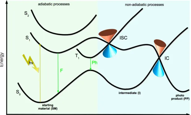
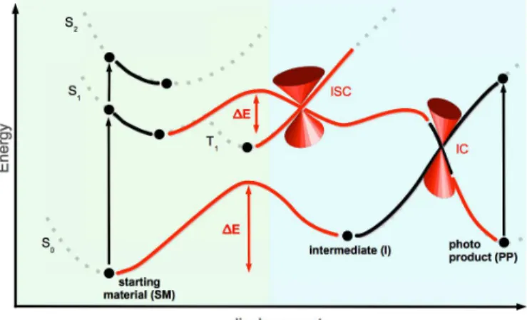
In Fig. 1.1 a one dimensional PES for a photochemical process is shown. Adia- batic and non-adiabatic processes are included in this picture. Without the direct knowledge of all the processes that are involved in a photochemical reaction, the topologies of the GS and the electronically excited states surfaces give already a lot of qualitative information about the photophysics of the investigated photo- system. Regions of interest are minimum energies and its associated geometries, transition states and conical intersections. As mentioned above, theoretical elec- tronic structure methods and experimental techniques complement each other.
This is particularly true for ab initio methods, which are entirely independent
Figure 1.1: One dimensional PES for a possible photochemical processes. The green shaded area shows adiabatic processes and photophysics. Fcorresponds to fluorescence, Ph to phosphorescence. The blue shaded area summarises all non-adiabatic processes.
The inter-system crossing (ISC) as well as the internal conversion (IC) occur in this example via a conical intersection (depicted by the typical double inverse cone shape, if plotted in a three dimensional PES).
from experimental input in contrast to empirical or semi empirical methods.
The introductiona of this work will therefore firstly focus on a short overview about the concept of potential energy surfaces (PES) and the theoretical methods on ab inito side used in this thesis as well as the combination of them with the molecular mechanic scheme (see Section 1.1). Afterwards, the general procedure for the investigation of the studied photocatalytical processes adopted in this work will be presented (see Section 1.2).
aThis content was already published conceptually as book chapter in [3, Chapter 14, p. 263et seqq.]. Parts of the text are identical to this chapter.
1.1 Excited states and computational methods
The understanding of photochemical reactions can be improved by using modern methods of computational or theoretical chemistry. Starting point for these meth- ods is the Schr¨odinger equation. One has to introduce approximations to solve the Schr¨odinger equation with more than one particle. The very first approximation for this problem is the so called Born-Oppenheimer approximation4 or adiabatic approximation. It allows the splitting of the molecular wave function into its nu- clear and electronic components due to the relative mass of the nucleus against the electron. Out of this approximation the concept of potential energy surfaces is derived. It describes the nuclear motion determined by the motions of electrons.
The understanding of the topology of the surfaces maps directly to properties of (photo-)chemical reactions. For the electronic part of the Schr¨odinger equation more approximations have to be introduced due to the electron-electron interac- tion and the high dimensionality. Here different approximations and methods can be used and are the starting point for the research field of quantum or theoretical chemistry. Since that in this thesis a lot of these principles have been used for the interpretation of the gained results, it is useful to highlight the above mentioned facts in a more extensive way. Of course, the subsections about potential energy surfaces and the computational methods make no claim to be complete. It is not the purpose of this part to give a detailed insight into these methods. Therefore the reader will find literature highlighting the topics much more detailed in the subsections.
1.1.1 Potential energy surfaces
The concept of potential energy surfaces (PES) directly results of the Born Oppen- heimer approximation.4 Because preparative chemists are reluctant to deal with complicated mathematical or physical equations, they use a much simpler argu- ment or model to describe this general principle. It is called reaction coordinate diagram, which shows the energy changes taking place during some mechanism.
The reactants are converted into the products by passing the reaction path through
a maximum energy state, the so called transition state. This diagram converts the potential energy surface of the molecules participating in the reactions into e.g. a one dimensional plot (see also Fig. 1.1). In principle, this is already a 1-dim PES.
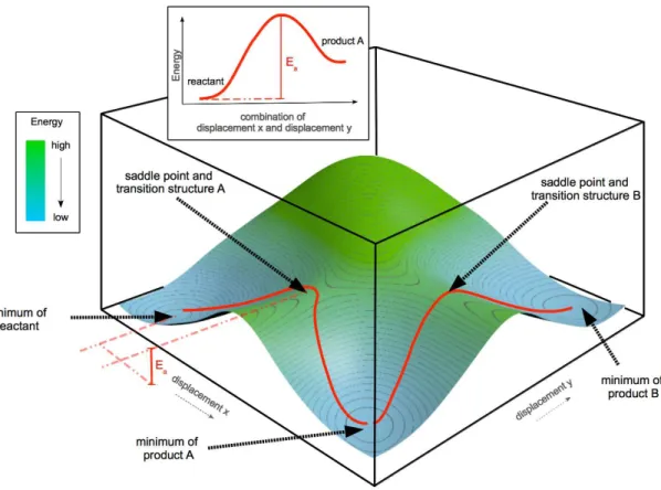
It describes the energy of the corresponding state of molecules as a function of the positions of the nuclei. Of course, the complete surface is 3N-6 dimensional (3N-5, if the molecule is linear), where N is the number of nuclei. As already mentioned, the topology of the PES directly maps onto chemical properties of the whole system. Minima represent stable structures and first order saddle points correspond to transition states. The connection of the potential energy surfaces and a reaction coordinate diagram is shown in Fig. 1.2.
Figure 1.2: Two dimensional (2-dim) PES with two reaction pathways starting from the reactant to product B passing product A. Additional the reaction coordinate diagram for the reaction to Product A is given. In both cases, Ea corresponds to the reaction energy.
In this figure, one global minimum, which represents the reactant of the given
system, and two local minima, representing products A and B, are shown. The reaction paths, depicted as red lines, connecting these minima via the two saddle corresponding to transition states.
Of course this concept can also be applied for excited molecules. In this case one would have two surfaces, one for the ground state and one for the excited state, the latter lying above the GS PES. For the adiabatic regime, which means that the two PES are sufficiently separated, the Born Oppenheimer approxima- tion works fine. Unfortunately, non-adiabatic coupling elements are neglected by this approximation. At points where two PES intersect, the energies of the two states are degenerate. At these points, small displacements in the nuclear coordi- nates change the character of the wave functions of the two states fundamentally.
Consequently, the two related wave functions describing a molecule at a conical intersection are arbitrary mixtures of the wave functions of the separated pure states. The non-adiabatic coupling elements thus become large and the Born Oppenheimer approximation breaks down. At these very interesting points, the motion of the electrons and nuclei is coupled. Therefore the system can cross the two PES very easy, efficient and fast which can be used in several ways. One prominent example is the photostability of the DNA. Conical intersections be- tween electronically excited states and the GS are used by nature to rapidly shed energy and to avoid photochemical reactions in photo-excited nucleobases.5 Con- ical intersections, postulated already in the 1930s,6, 7 have become ubiquitous in photophysics during the past two decades. For a non-linear three-atom molecule like ozone8 the PES of two states touch in a single point. Due to this topology, it is often illustrated as a double inverse cone.9 For bigger molecules the space of degeneracy corresponds to a 3N-8 dimensional hypersurface (there are two addi- tional conditions to be fulfilled such that the two by two CI matrix involving the two relevant states yields two degenerate eigenvalues).
The exemplary presented photochemical reaction in Fig. 1.1 shows the main adi- abatic and non-adiabatic reactions that are possible after excitation and they are now in the centre of attention. The absorption from the GS (or S0) to the first singlet state occurs in the time range of femtoseconds. After the relaxation to the
lowest vibrational level, the molecule can get back to the ground state by emit- ting a photon. This is called fluorescence (F), which is happening in nanoseconds range. The emission of a photon out of a triplet state is called phosphorescence (Ph). This process takes place in the milliseconds time range. All these are adi- abatic processes. On the other hand, processes with no radiation of photons as well as the population of other spin states (e.g. triplet states), which are very important in photochemical reactions, are governed by non-adiabatic processes.
Crossings of surfaces can occur between same or different spin symmetries. If the crossing involves states with different spin symmetry one speaks of inter-system crossing (ISC), otherwise of internal conversion (IC). If the IC is based on vibronic coupling, the process is also an adiabatic one. However, both cases decrease the fluorescent quantum yield. Ultra fast conversion, for instance to the photoproduct in Fig. 1.1, is often mediated by a CI between two surfaces.
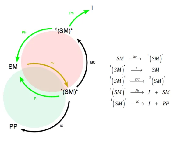
The exemplary photoreaction from Fig. 1.1 can be reduced schematically to the following very simple overall reaction formula:
In this overall reaction the reactant (SM) is converted to an intermediate (I) and the photoproduct (PP) after excitation. It does not play a role, whether the reaction is based on a monomer or a complex reaction of a lot of starting materials to a desired photoproduct. The reaction coordinate would be the displacement of the system e.g. along some internal coordinate in this example. Due to the knowledge of the shape of the PES (see Fig. 1.1) one can discuss this reaction more detailed. After the excitation of the starting material into the first singlet state one possible relaxation would be the fluorescence back to the GS. But also ISC into the first triplet state could occur to some extent. In this case, the process would be non-adiabatic, mediated by a conical intersection. A deactivation channel back to the starting material or to some intermediate is phosphorescence. The productive channel to the photoproduct would be the IC by a CI from the first singlet state.
All these processes can now extent the simple reaction formula from the beginning to a valid ”photocycle” and extended formulae, which are shown in Fig. 1.3.
Figure 1.3: Corresponding photocyle to example reaction (see Fig. 1.1) and extended reaction formula. The green cycle is productive, the red one is destructive.
Of course, all reactions still depend on the one hand on the energetic barriers, which have to be passed during the reaction pathway and on the other hand on displacements which are necessary for the forthcoming of the reaction. Neverthe- less, the knowledge of the character of the involved PES as well as the conditions for non-adiabatic processes in the photochemical reaction is of benefit for the tun- ing of reactions towards a desired photoproduct. Quantum chemical methods and theoretical chemistry can be part of the investigation of these problems and help for the description of reasons for unexpected intermediates or failed photoreac- tions. In the following, two classes of quantum chemical methods often used for such purposes are presented.
1.1.2 Computational methods
The description of electronically excited states with ab initio wave function methods can either be done by using time dependent density functional theory (TD-DFT), or single as well as multi-reference methods. The latter ones are difficult to use in the applications to extended molecular systems and will not be discussed here, as they were not used in the context of this thesis. However, detailed information about these methods can be found in the literature.7, 10 Single reference methods include methods like Configuration Interaction, e. g. the Configuration Interaction Singles CIS11 method, propagator methods like RPA and ADC,12, 13 and time-dependent coupled cluster response TD-CC methods.
TD-DFT and TD-CC both have in common, that they are response methods, which means, that excitation energies are calculated as the poles of the time- or frequency dependent polarizability by first-order perturbation theory (linear response). It is based on a time- or frequency-dependent external perturbation and thus excitation energies can be regarded as a time or frequency dependent ground state property of the studied molecule. In the following, the main focus is on TD-CC and TD-DFT, because these methods are inexpensive enough to describe issues in photocatalysis and were used extensively in this thesis. Addi- tional to that, special attention will be given to potential pitfalls. For detailed information, the reader is referred to the references given during the next few lines.
Starting with TD-CC, one should begin with the equation for the coupled cluster wave function. It is specified by an exponential excitation operator acting on the Hartree-Fock reference wave function |0i:
|CCi= exp(T)|0i (1.1)
T =X
i
Ti (1.2)
Approximations can be done by truncation of the sum of T (see Equation 1.2) , the cluster operator, e.g. for coupled cluster singles and doubles, where i = 2.
The two resulting cluster operators T1 and T2 each generate a linear combina- tion of all possible singly and doubly substituted determinants, respectively, from
|0i . Singly substituted means that a certain molecular orbital occupied in the reference is replaced by a virtual molecular orbital and doubly that two certain molecular orbitals are being replaced by two virtual molecular orbitals, respec- tively. As one can see from Equation 1.1 there is an exponential ansatz for the wave function. Due to this fact, the wave function is always (at each truncation level) product separable and the energies are thus size extensive. Furthermore, all possible excitations of full configuration interaction are generated, even when the cluster operator is restricted to only singles and doubles as above. The co- efficients of higher excitation levels, like quadruples, then factorise as products involving singles and doubles coefficients.
So far, the method is highly accurate to describe ground states and provides a large fraction of the correlation energy.14 To describe excited states within the couple cluster framework commonly applied methods are the equation of motion couple cluster (EOM-CC) methods15 and time dependent coupled cluster (TD-CC) linear response16, 17 based on the hierarchy of the coupled cluster models CC2,18CCSD, CC3,19and CCSDT. The TD linear response approaches aim at the frequency dependent polarizability of the system by first-order perturbation the- ory, which means that the excitation energies are calculated as the poles, and the transition strengths as the residues of this time-dependent ground state property, as mentioned above. TD-CC2 response is the cheapest method including dynamic correlation effects in the given hierarchy. The reason for the inexpensive character of this method is that similar to second order Møller–Plesset perturbation theory (MP2) doubles substitutions are just treated to first order w.r. to the fluctuation potential. Despite of this simplification, TD-CC2 is quite a robust method and provides a qualitatively correct picture of excited states with an accuracy of about 0.2–0.3 eV in the excitation energies compared to experimental values. But, this accuracy is limited to excited states that are dominated by singles substitutions, which is usually the case for low energy excitations as those considered here. In the vicinity of CI, the excitation energies may become complex, though there are correction schemes to cope with that problem.20 However, any response
theory has this drawback and breaks down for conical intersections with the ground state, since at this point the ground state reference no longer is properly described by a configuration state function. On the other hand, the most impor- tant drawback of TD-CC response is the restriction to rather small molecules, especially for the description of electronically excited states. This is also true for the comparatively cheap TD-CC2 response method, particularly so for energy gradients w.r. to nuclear displacements, as needed for geometry optimisations on excited state surfaces. A practical approach, which was also applied in this thesis, is to utilise the cheap TD-DFT methods for geometry optimisations and TD-CC2 for excitation energies and other properties at these TD-DFT geometries.
This leads to Kohn–Sham density functional theory (DFT), which is one of the most frequently used theoretical approaches in almost every field of chemistry.
According to the Hohenberg–Kohn theorem21 there exists a functional E[ρ(r)]
mapping the exact electron density to the exact energy. That means, the energy can in principle be calculated using a much simpler object than a wave function, the so called (one-particle) density function ρ(r), which depends only on three degrees of freedom. Unfortunately, nobody knows what this functional actually looks like, because the Hohenberg–Kohn theorem just proves the existence of it.
The unknown part of E[ρ(r)] can be condensed in the exchange correlation part Exc[ρ(r)]. This part has to be modelled, which is why present DFT functionals are semi-empiric approaches. This approximation led to a plethora of different Exc[ρ(r)]. They range from simple local density approximations (LDAs), over gra- dient corrected functionals (GGAs), hybrid functionals like the famous B3LYP,22 to range-separated hybrids, orbital dependent functionals, and random-phase ap- proximations for correlation. To describe electronically excited states, a linear response theory on the basis of DFT is mostly used in TD-DFT.23 The famous Casida’s equations are very similar to those of time-dependent Hartree–Fock the- ory and as for TD-CC response, the excitation energies correspond to the poles of the frequency dependent polarizability. The TD-DFT methods are very effi- cient methods for excited states, especially for extended systems. In comparison to ab initio wave function methods, the analytical gradients and thus geometry
optimisations are very inexpensive. This general simplicity in the usage and the availability in most ab initio electronic structure program packages, are probably the keys to its enormous success. On the other hand, both DFT and TD-DFT lack the possibility of a systematic improvement of the method, since there is no such hierarchy of methods as for ab initio wave function methods. Another draw- back of the method are artifacts plaguing DFT, like a non-vanishing correlation energy of a single electron or the self-repulsion of electrons. The latter has se- vere consequences for TD-DFT. The excitation energies of charge transfer (CT) excited states are grossly underestimated24–26 due to the absence of the excitonic hole-particle attraction in local or semi-local functionals.27 Large separation of hole and particle in the excitation energies of CT excited states lead to an un- derestimation of the energies by several eV. Additionally, these states also mix eventually with other low-lying valence states and contaminate them. To some extent, hybrid functionals with a large fraction of non-local exchange or range- separated hybrids28–30 shift CT states back to higher energies. Even the TD-DFT response method is unable to deal with conical intersections, just like the TD-CC methods. These drawbacks have to be in mind, when applying TD-DFT, foremost if low-lying CT states appear. Often those states are absurd and may even con- taminate other valence states, which leads to a wrong picture of photophysics of the investigated system. Verification of the TD-DFT calculations with methods like TD-CC2 are crucial to avoid this issue.
1.1.3 QM/MM scheme
Although, TD-CC and TD-DFT methods are inexpensive enough to describe pho- tochemical reactions, addition of solvents or large biologic systems make them inefficient. So, combination of QM-methods with the less expensive molecular mechanic (MM) method is desirable. In the 1970s of the last century, Warshel and Levitt first suggested to combine these two methodologies,31which has become famous as the QM/MM hybrid approach. Their trendsetting idea had already all in hand, which is still used nowadays. Field, Bash and Karplus were the first who combined the CHARMM force field, a widely used model potential for MM
calculations, with QM methods.32 This idea was honoured with the Nobel Prize in chemistry in the year 2013.33, 34 For the QM/MM approach, the whole system (S) is divided in two parts (regions). The first part (QM-region, I) is in almost every case very tiny with respect to the rest and consequently can be treated with accurate and appropriate QM methods. It comprises the part of the system, in which the actual reaction takes place. The second and larger part (MM-region, O) holds the rest of the studied system. In Fig. 1.4 this is shown schematically.
Figure 1.4: Complete system S divided into outer O (red) and inner part I (green);
region between Oand Iis depicted in magenta and contains the possible link atoms L.
Due to the fact that only a small part of the complete system is treated with an expensive QM method in contrast to the MM region, it is possible with the QM/MM approach to investigate truly large systems. Inclusion of only the interesting parts in the QM-region, e.g. the enzymatic active region of a protein, or, if the method is utilised for the description of solvation effects, one single solute molecule or alternatively, a cluster of the solute with its first solvation shell, reduces the computation time dramatically relative to a full QM treatment of the whole system, which would be entirely unfeasible. Since solvation severely affects reactions and, especially in photochemical reactions, photophysical properties of molecules, the QM/MM approach is an excellent tool to be employed to describe these effects and taking them into account for the investigations of reaction mechanisms. The MM methods, often simply called force field methods, can be used to mimic the natural environment, which in biological systems is water.
There are a lot of different model potentials for water; the most prominent one is the TIP3P model.35 It is a 3-site water molecule parametrised to reproduce
the behaviour of liquid water. This model has been improved by a lot of other approaches. Organic systems on the other hand are often non-polar and cannot be solved in water and therefore non-polar solvents have to be used for these systems. Yet, for the MM scheme in principle every solvent can be modelled and used in the QM/MM calculations. After this short motivation an overview of the model potentials or force fields, as employed in MM methods, is given.
Subsequently, the coupling of the MM and QM methods and the resulting traps related to this coupling are discussed to some extent.
Major application of the MM methods is in the framework of biology. Calculations of the energy of such systems within this approach only depend on its atomic coordinates. The energy and the forces on the atoms are related to the gradient of the potential function. This function sums harmonic contributions originating from bond- and bond-angle-displacements, cosine terms reflecting displacement of dihedral angles (torsions), as well as electrostatics (modelled by partial charges or higher moments), van-der-Waals dispersion and exchange repulsion terms. In Equation 1.3 an example of a simple potential is given.
EMM =Ebonded +Eunbonded (1.3)
Ebonded =Ebond+Eangle+Etorsion (1.4) Eunbonded =Evan-der-Waals+ECoulomb (1.5) Splitting this up, the bonded energy termsEbonddescribes the interaction between two atoms and is given by the following equation:
Ebond= X
bonds
kd(d−d0)2 (1.6)
It sums up all existing bonds between two atoms, where kd is the force constant, which describes the type of the bonds (e.g. single or double bond of two carbon atoms) and d0 is the equilibrium distance.
The angle between three atoms is considered by Eangle and given in Equation 1.7.
As before, a force constant kθ and an equilibrium angle θ0 are part of the energy term.
Eangle = X
angles
kθ(θ−θ0)2 (1.7)
In an analogous way, torsions between four atoms are described by
Etorsion = X
torsions
kφ[1 + cos(nφ+δ)] (1.8) Non bonding interactions are included by van-der-Waals and Coulomb terms (see Equation (1.9))
Eunbonded = X
unbonded pairs AB
( ǫAB
"
σAB
rAB 12
− σAB
rAB 6#
+ 1
4πǫ0
qAqB
rAB )
(1.9)
For the following discussions the description above should be sufficient and the reader should now have a feeling how this potentials are built. For a detailed review of force fields and all related issues the reader is referred to an excellent review article of Ponder and Case.36 Outgoing from these equations it is evident that quite a lot of parameters affect such a model potential. They constitute the so called force field and different parametrisation certainly lead to different force fields. The development of the needed parameters is quite complicated and needs a lot of knowledge. This also results in a careful integration of new molecules, not covered so far to a specific force field. The combination with QM methods for the combined QM/MM approach allows for almost every force field to be used. The two established ones are AMBER37 and CHARMM.38, 39 They can be attached to almost every problem and are optimised for biological systems like enzymes, proteins and DNA. However, it is possible to use them also for other chemical studies. The first mentioned AMBER force field also offers the possibility to parametrise organic molecules within its framework by using the GAFF (general AMBER force field) parameters,40 which was used in the framework of this thesis.
The GAFF force field parameters are designed for compatibility with the original AMBER force field developed for biological systems. GAFF includes parameters for almost every organic or pharmaceutical molecule composed of hydrogen, carbon, nitrogen, oxygen, sulphur and phosphorus. A common procedure to import molecules is available and described by Bayly et. al.41 Nevertheless, there are also force fields, that were developed especially for small organic molecules and are therefore more versatile because of a higher diversity. Specialised force fields like MMx,42–44 UFF45 should be mentioned in this context and are used quite extensively. Gromacs46also provides this alternative for the sake of completeness.
As already mentioned at the beginning of this section, the combination of the QM and MM methods leads to the QM/MM hybrid approach. MM methods are used for the surrounding, like solvents or larger parts of proteins, of the region of interest, which is treated by the QM methods. As one can see schematically in Fig. 1.4, the whole system S is divided into I (QM-region) and O (MM-region).
Each atom of the system is assigned either to O or I. The coupling of those two parts is an important step and determines also the accuracy of the QM/MM calculations, besides the method of choice. In principle this can be done in two different coupling schemes, (i) the subtractive (see also Equation (1.10)) and (ii) the additive (see Equation (1.11)) coupling. Both schemes are well developed in the meantime and discussed in detail in a lot of articles and reviews.47–50
For the subtractive coupling (i) the energy of the whole system S is calculated by the force field (EM M(S)) at first, followed by separate MM and QM calculations for the energy of the subsystem I (resulting in EQM(I+L) and EM M(I+ L).
Subtracting EM M(I+L) from the sum of EM M(S) and EQM(I+L) leads to the QM/MM energy of the system.
EQM/M M(S) =EM M(S) +EQM(I+L)−EM M(I+L) (1.10) Implementation of this scheme is quite simple, but leads to some errors due to the fact that the polarisation of the QM part by the MM part is not taken into account. For the additive scheme (ii) the MM calculation is only performed for
the MM part (EM M(O)), followed by a QM calculation for the energy of the inner region (EQM(I+L)). Now a special coupling term (EQM−M M(I,O)) is needed to describe the interaction of the two subsystems. Addition of these three energies yields the QM/MM energy of the whole system.
EQM/M M(S) =EM M(O) +EQM(I+L) +EQM−M M(I,O) (1.11) Before the coupling term EQM−M M(I,O) is briefly discussed, the reader may have recognised the abbreviationL. For the case thatIandOare not connected to each other via a chemical bond, no further challenges for the QM/MM calculations arise.
In most cases, especially if the system comprises of proteins, it is not possible nor appropriate to divide S into subsystems without artificial bond breaking. That artificial bond break has to be capped with appropriate procedures otherwise homolytically or heterolytically cleaved molecules in the QM or MM region would lead to artificial radicals or charges, which have little relation to the original system. For this problematic issue different solutions were developed. One variant is to introduce additional atoms to the QM region, covalently bound to the last QM atom. This scheme is called the link-atom scheme and is achieved by capping the atoms with hydrogen or fluorine atoms.51 Another possibility is to add localised orbitals at the boundary, which are kept frozen in the QM calculations.52 There are further methods to handle this problem, which are not discussed here; the reader is therefore referred to the excellent review of Senn and Thiel about the QM/MM scheme in general.53 In particular for the link-atom scheme one has to be careful to prevent over-polarisation of the QM density.54 However, throughout this thesis, the link-atom approach was used with care, knowing its drawback, due to its simplicity.
Coming back to the EQM−M M(I,O) term, once again, different solutions were developed:55 (i) the mechanical and (ii) the electrostatic embedding should be mentioned here. The mechanical embedding is based on MM-MM electrostatics, while electrostatic embedding implies inclusion of MM charges in the QM calcu- lation: the MM point charges are included in the one-electron Hamiltonian of the QM region as sources of an external electrostatic field. With this procedure the
polarisation of the QM part through the MM part is taken care of.
1.2 General Procedure
After this short elemental introduction, the procedure, which was used for the investigation of photochemical systems and photocatalysis, is presented. One should mention that it is quite difficult to give a general recipe for QM or QM/MM investigations dealing with these tasks. However, the used procedure covers the most important aspects for the description of such investigations, but it is essential to have the discussed pitfalls and drawbacks in mind: it starts with the proper choice of the QM method and ends with the final interpretation of the results.
During the study of different systems and aspects in this thesis, in principle two steps must be considered to get reasonable results. These two steps showed to be quite robust. If one is interested in the conical intersection seam, further and not straightforward calculations have to be done. These further procedures are not discussed here and were not part of the investigations made in this thesis.
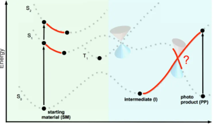
To make this procedure more clearly, the example of a photochemical reaction shown in Fig. 1.1, which is used almost throughout this introduction, was taken to visualise the important aspects. The original reaction is shaded while the actual steps are coloured red. Black depicts already gained information.
1. The starting point of every theoretical investigation of an arbitrary system is the vertical excitation spectrum for the ground state minimum (FC-point).
This is only one first jigsaw piece for the complete investigation. At that point the types of all electronically excited states have to be determined.
Different methods should be compared and calibrated at that stage, e. g.
TD-DFT with different functionals should be compared to TD-CC2 reference calculations. This provides the needed information, which method or func- tional can be applied for the target system (this is strongly recommended for QM/MM investigations in order to use the affordable TD-DFT methods).
Figure 1.5: Step 1.1: Vertical excitation spectrum for the ground state mini- mum, assignment of the types of the electronically excited states and validation of methods (not shown schematically).
Next, the relevant low-energy minima on the PES of the excited states have to be determined. With the geometries related to the reactants, interme- diates and products of a photochemical reaction at hand, one already has a qualitative picture of the mechanism at work. A practical approach as mentioned before, is to utilise the cheap validated TD-DFT methods for geometry optimisations and TD-CC2 for excitation energies and other prop- erties at these TD-DFT geometries.
Figure 1.6: Step 1.2: Geometry optimisations of low-energy minima on PES of excited states for SM, I and/or PP.
2. In order to determine the minimum energy path between reactants and prod- ucts is more intricate: Provided that the reaction coordinate is a priori known, i. e., reflected in one or just a few internal coordinates, geome- tries along the reaction coordinate can be generated by hand. Otherwise more general and costly approaches must be utilised. For example, the NEB (nudged elastic band) method56 could be used. For a detailed discussion about optimisation methods to determine minimum energy paths the reader is referred to the literature.57
Figure 1.7: Step 2: Determination of minimum energy paths of involved species.
1.3 Outline
After this introduction, three examples for the investigation of photochemi- cal/photocatalytical issues with the above shown scheme are presented. The first one deals with roseoflavin, a photocatalyst, which is suitable to replace the well known flavin as photochromophore in biological systems as well as in chemical photocatalysis. This study shows the general applicability of the used scheme by comparing them to available photophysical investigations (see Chapter 2). The second example deals with two artificial dinucleotides consisting of a nucleoside with benzophenone as chromophore and of one of the two natural nulceosides guanosine and thymidine, respectively. The objective was to investigate a possi-
ble photo-induced intramolecular charge transfer in detail (see Chapter 3). The third and last investigation covers a step in a proposed reaction mechanism of visible light mediated photochemical decarboxylations (see Chapter 4).
In the presented examples, TD-DFT was used for geometry optimisations of elec- tronically excited states in most cases. In order to identify potential problems, like contamination of relevant valence states by low-lying charge transfer states, TD- CC2 single point calculations were always performed to be aware of this pitfall.
The two methods were compared with each other by comparing the singles sub- stitution vectors, as well as dipole moments and transition strengths. If the time saving TD-DFT methods were insufficient for the solution of the given systems, the more robust and qualitative correct TD-CC2 method was used.
For some of the presented examples, solvent effects were taken into account by using the described QM/MM scheme. Parametrisation for the molecular force field was done very carefully. Solvated geometries for the QM/MM calculations were generated on the basis of minimum energy structures of isolated solute (op- timised by using QM methods) embedded in a large enough solvent shell and by performing MD simulations after an initial equilibration phase. The typical MD trajectories range between 500 psand 10 ns, depending on the size of the system.
Subsequently, different snap shots representative for the relevant geometries en- countered during the MD simulation were chosen as starting points for following QM/MM investigations on the ground and excited state surfaces.
The content of this chapter has been published in Physical Chemistry Chemical Physics.58 Parts of the text are identical to the publication. Besides some changes in formulations the publication was revised concerning the context given in this thesis, i.e. basic principles, which were discussed in Chapter 1, and the appendix of the publication was integrated into the text to some extent.
2.1 Introduction
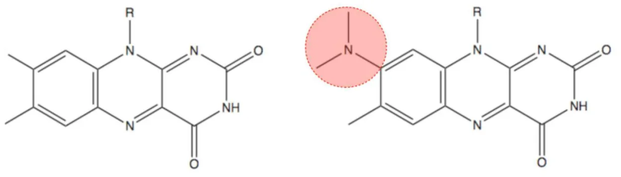
To use flavin (see Fig. 2.1) as photocatalyst in organic chemistry is an obvious idea.
Riboflavin or vitaminB2 (see Fig. 2.1,R= ribityl group) is an important biological redox cofactor and is involved in a large number of processes as photoreceptor to perceive light at a strong absorption up to 500 nm. Riboflavin is the central com- ponent of the flavin mononucleotide (FMN or riboflavin-5’-phodsphate) or flavin adenine dinucleotide (FAD) used in bacteria, plants and mammals as photorecep- tor. If these photoreceptors are incorporated in proteins, they are called BLUF (blue light using FAD)59 proteins. The first discovered BLUF protein containing such a domain was AppA from Rhodobacter sphaeroides.60–66
Since the first discovered BLUF-domain containing flavoprotein several other BLUF signalling domains have been found in prokaryotic and eukaryotic microor- ganisms.67 These include BlrB,68, 69 Slr169470–74 and Tll0078.75–77 Most of them have different physiological functions, but share a common feature, namely the change in their UV/Vis-, as well as in their IR-spectra upon signalling state for- mation. It is therefore widely accepted that different BLUF domains should have
Figure 2.1: Chemical structure of flavin (left side) and roseoflavin (RoF; right side; dimethylamino group (DMA) depicted in red). R depicts possible side chain of molecules.
the same or similar mechanism for the signalling state formation. The lack of unique crystal structures for both the dark- and light-adapted forms of BLUF- domains however has made the search for a conclusive mechanism of signalling state formation a challenge. A lot of proposals for this were made so far. Many different mechanisms were postulated,78–83 which all have in common the very first step, i.e., an electron transfer process from the nearby tyrosine residue to the flavin chromophore, which explains the observed fluorescence quenching of the latter. Sadeghian et. al. presented a plausible mechanism for the formation of the signalling state based on a systematic investigation of the potential energy surface.84, 85 There is strong evidence that after photo-excitation of the locally excited (LE) state of flavin, the tyrosine → flavin charge transfer (CT) state is populated via a conical intersection.
This conical intersection seam has been investigated in detail by Udvarhelyi and Domratcheva.86 At the level of the complete active space self consistent field (CASSCF) method the authors located the minimum energy point on the seam along the relevant proton transfer reaction coordinate. Moreover, they also calcu- lated pathways for the entire photo reaction leading to the final signalling state structure. The steps of this reaction cascade include tautomerization of the highly conserved glutamine residue and are in principle in agreement with the ones pos- tulated by Sadeghian et. al. .
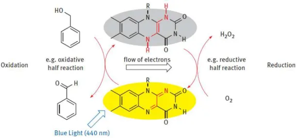
However, as mentioned before, flavin itself can also be used successfully in organic photochemical reactions as photocatalyst for redox reactions. One example for such a photocatalytic reaction is the oxidation of methoxybenzyl alcohol to an aldehyde.87 In Fig. 2.2 the scheme of the oxidation mechanism is depicted, which was proposed utilising transient absorption spectroscopy among other techniques [3, Chapter 15, p. 295 et seqq.].
Figure 2.2: Catalytic cycle of flavin redox reactions. Benzyl alcohol oxidation and reoxidation of the catalyst by air [3, Chapter 4, p. 47].
It was shown that after the excited state of flavin is quenched by an electron transfer step, the reaction proceeds via the triplet states of the occurring species of methoxybenzyl alcohol and its intermediates generating the desired aldehyd.
Furthermore, electron transfer on the singlet excited state side is a loss channel for the desired reaction.88
In order to diversify the catalyst, interest came to roseoflavin (RoF). RoF has in addition to the flavin skeleton a dimethylamino group (DMA) as modification (see also Fig. 2.1). This leads to a possible new chemical photocatalyst with different properties.
Coming back to proteins, replacing the FAD moiety by a roseoflavin-analog, the understanding of the wide and controversial discussed proposals, briefly discussed
before, about the mechanism for the signalling state formation in BLUF proteins could be verified. And indeed, Mathes et. al.89 replaced the FAD chromophore of wild type Slr1694 BLUF domain with a domain in the protein containing RoF to get a deeper general insight in the formation of the signalling state. The main observation from these experiments is the lack of the photocycle and with that the loss of the biological function of the protein by the flavin → RoF exchange.90 Additionally to that, the behaviour of RoF in different aqueous and organic sol- vents was also investigated by Zirak et. al.91 There is evidence that RoF might not work as a potential new photocatalyst.
2.2 Motivation and Results
Since there are many experimental studies, reliable results and proposed mecha- nisms for a photophysical deactivation by intramolecular charge transfer processes for RoF, the general procedure described in the introduction was used to investi- gate the photophysical properties more detailed on basis of theoretical calculations.
For the isolated RoF as well as for RoF solvated in water, the general usability as photocatalyst can be answered by theoretical methods using also the QM/MM scheme. Possible deactivation processes discussed in the literature can be con- firmed or rejected and give a new insight into this interesting theme. Also the loss of the biological function of the protein was studied by using QM/MM techniques.
Therefore this section is divided in three parts: (i) the study of RoF as isolated molecule, (ii) RoF surrounded by a water environment and (iii) RoF incorporated in the BlrB protein. Throughout this investigation, all QM calculations were done using the TURBOMOLE92 program package.
2.2.1 Isolated roseoflavin
The first important point to begin with was the determination of the GS geometry of the RoF molecule in gas phase. The orientation of the DMA group relative to the isoalloxzine ring system is crucial, since this is the main difference between
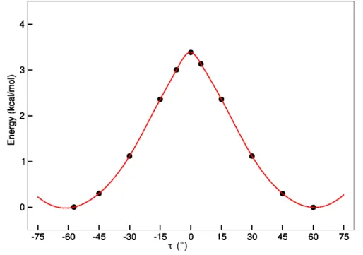
RoF and flavin and could also have some influence inserting this moiety in a protein environment. Therefore a relaxed energy path along the dihedral angle τ (illustrated in Fig. 2.5) was calculated. For the QM calculations of an isolated molecule DFT (using the BHLYP93 functional) and def-SVP basis94 was applied.
Figure 2.3: RoF in the gas phase : relaxed energy path along the dihedral coordinate τ (see Fig. 2.5) at the level of DFT (BHLYP functional/def-SVP basis)
As one can see in Fig. 2.3, a minimum energy is reached with a dihedral angle of τ ≈ ±60◦ between the DMA group and the isoalloxazine ring system. For the RoF molecule in gas phase the DMA group is kind of electronically decoupled to the ring system, because the DMA group is not in plane with the ring system.
For the gained minimum geometry in the ground state for τ ≈ −60◦, vertical excitation energies were calculated with different TD-DFT functionals (BP86,95 B3LYP22 and BHLYP) with def-SVP basis as well as TD-CC218, 96, 97 with stan- dard auxiliary basis sets,98RI approximation99and the def-SVP and aug-cc-pVDZ basis sets.100 The calculations did not aim only for the excitation properties of the molecule, but also for the quality of the different TD-DFT functionals and their applicability for further investigations, especially for the BLUF protein. The
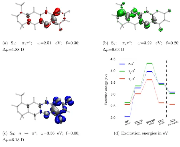
electronic density difference plots and the corresponding oscillator strengths for the first three states were also obtained by the calculations with TD-CC2/aug- cc-pVDZ. They are shown in Fig. 2.4, together with a schematic picture of the excitation energies for the different methods.
(a) S1; π1π∗; ω=2.51 eV; f=0.36;
∆µ=1.88 D
(b) S2; π2π∗; ω=3.22 eV; f=0.20;
∆µ=9.63 D
(c) S3; n → π∗; ω=3.36 eV; f=0.00;
∆µ=6.18 D
(d) Excitation energies in eV
Figure 2.4: (a)-(c) TD-CC2 density differences (w.r. to the ground state, aug-cc-pVDZ basis) of the first three excited states of RoF. The blue, red, and green isosurfaces at
−0.004 show the regions with loss, the grey ones at +0.004 the regions with gain of electron density upon photo-excitation. The corresponding oscillator strengths f (on length representation) and the change of the dipole moment ∆µ are denoted as well.
(d) Vertical excitation energies of RoF in the gas phase calculated with TD-DFT and TD-CC2 response, respectively.
With the corresponding electronic density difference plots and oscillator strengths,
calculated with TD-CC2, the character of the first three excited states were de- termined (see Fig. 2.4(a) to Fig. 2.4(b)). The S1 state is of (π1π∗) type, the S2
state of (π2π∗) type and the S3 state is a (nπ∗) state.
The methods per se predict different energetic orders for the (ππ∗) and (nπ∗) excitations, as is evident from Fig. 2.4(d). With the exception of the BP86 functional, the (π1π∗) state is the lowest state. The position of the (π2π∗) and (nπ∗) states differs from TD-DFT to TD-CC2. This is in dept to the inherent self interaction error26, 27 of TD-DFT’s local and semi-local functionals. From the dipole moment changes relative to the ground state (∆µ) it is obvious, that these states have a little charge transfer character.
The (π1π∗) state, which is the HOMO →LUMO excitation, features the highest oscillator strength and therefore is most likely populated after photo-excitation.
Further investigation of this state was done by optimising the geometry at TD- CC2 level. At the fully relaxed geometry, the S0 → S1 transition maintains its (ππ∗) character. The second and third excited states, with (π2π∗) and (nπ∗) char- acters respectively, switch their energetic order. The energy difference between the (π1π∗) and (nπ∗) state drops from 0.85 eV to 0.52 eV at the (π1π∗) minimum.
The major geometrical changes during the optimisation at the S1 PES correspond to particular bond distances in the RoF ring system. The orientation of the DMA group on the other hand is not affected by this relaxation process. The changes in the bond distances were starting point for a more accurate study of this issue. An appropriate linear combination of these bond distances was constructed as a reac- tion coordinate QR for this purpose (see Fig. 2.5 QR = α×b(O2-C2)−α×d(C2- N1)+α×d(N1-10a)−α×d(10a-4a)+α×d(4a-N5), whereas α = 0.4472). For sim- plicity the bond distances were not wighted at all. A free geometry optimisation with the constructed linear combination of the bond distances has shown that the global minimum of the S1 state corresponds to QR = 0.46 and the minimum geometry along the QR path, with QR = 0.45, are energetically 0.0001 eV and geometrically 0.01 a.u. (RMSD) apart.
A relaxed energy path on the PES of the lowest state was calculated at the TD- CC2 level with def-SVP basis along the reaction coordinate QR, starting at the
Figure 2.5: Reaction coordinate QR. Elongation of bond is denoted in green, con- traction in red. The used dihedral angles τ and τ’ correspond to (C7,C8,N8,C8L) and (C7,C8,N8,C8R), respectively.
FC-point. This path is displayed in Fig. 2.6.
One can see that the path along QR leads to a CI between the (π1π∗) and the (nπ∗) state. After the CI the (nπ∗) state becomes the lowest state. The step in the energies after this CI between (π1π∗) and the (nπ∗) state is due to the change in geometry of the optimised structure, since the restrained optimisation refers to the lowest state. Continuing the path along QR now on the (nπ∗) state surface, one can observe even a second CI with the ground state. The switching of the energetic order of the (π2π∗) and (nπ∗) states, noted at the S1-minimum, seems to derive from a third CI between theses states.
The conclusion of the investigation so far is (i) a twisted structure of RoF for the ground state minimum and (ii) a fast deactivation channel from the photo-excited (π1π∗) state to the ground state via two CIs in the gas phase occurring via changes in bond distances of the RoF ring system. The DMA group is not affected in the observed CI. This study of RoF also showed that the BHLYP functional seems to be feasible for geometry optimisations of excited states, if using the cheap TD- DFT method. However, energies and corresponding properties should at least be verified by application of the TD-CC2 method.
Figure 2.6: Energies (in eV) of the relevant excited states relative to the ground state minimum energy at the relaxed structures alongQR. The restrained geometry optimisa- tions were performed with TD-CC2 response in the def-SVP basis on the energy surface of the lowest state, i.e., on the (π1π∗) surface and on the (nπ∗) after the conical inter- section. The plotted energies correspond to TD-CC2 response single point calculations at these relaxed structures in the bigger aug-cc-pVDZ basis. The shaded points denote the S1-minimum.
2.2.2 Roseoflavin in water
To solvate the RoF in water a pre-equilibrated water droplet of 25 ˚A diameter containing 2142 water molecules was used. An extensive MD simulation was not carried out. This part of the study served as an investigation of the influence of the water molecules, represented by ”partial” charges in the one-electron part of the QM-Hamiltonian. A MM-minimised structure was used as starting point for the subsequent QM/MM geometry optimisations. A boundary of 2.5 ˚A thickness to the outer limit of the droplet was restraint by a quartic force of 24 kcal/mol/˚A2 us- ing the miscellaneous mean-field potential (MMFP) implemented in CHARMM.39 The potential parameters for the RoF chromophore were taken over from the flavin chromophore.84 Missing parameters were adopted from the CHARMM27 force field parameters for nucleic and amino acids.38, 101 The list of additional force field parameters and a figure with the corresponding atom numbers and types are given in the appendix (see Fig. A.1, Table A.1, Table A.2 and Table A.3). The parameter for the water molecules were also taken over from the CHARMM27 force field parameters. The QM region was restricted to RoF, while the MM region contained the surrounding water molecules. For the QM/MM calculations, employed by using the ChemShell interface,102 the coupling between QM and MM was done via the charge shift scheme. The DL-POLY molecular dynamics package103 incorporated in ChemShell with CHARMM force field parameters was used for the MM part. The implemented HDLCopt-optimiser104in ChemShell was chosen for the geometry optimisations. DFT with the BHLYP functional with def-SVP basis set was used combined with the CHARMM force field parameters (BHLYP/CHARMM).
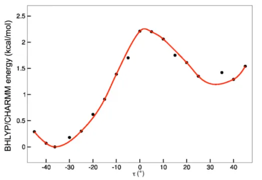
With the QM/MM technique a relaxed energy path (shown in Fig. 2.7) along the dihedral angle τ was calculated. As for the molecule in gas phase, the orientation of the DMA group of RoF embedded in the water environment is an important task to find out.
The stable conformation corresponds to two minima at τ ≈ ±35◦, which shows that the twisting is not that pronounced as in the free molecule. The asymmetry
Figure 2.7: BHLYP/CHARMM energies of RoF in water along the dihedral angle τ (defined in Fig. 2.1).
of the QM/MM energies with respect to τ for the two minima in Fig. 2.7 is due to a not fully relaxed solvent environment at the dihedral angleτ = +35◦. A sym- metric PES with respect to the dihedral angle τ would be obtained once the water environment is fully adapted to the restrained RoF residue. However, this exten- sive QM/MM MD simulations was avoided, due to the fact, that only the question about the general orientation of the DMA group should be answered qualitatively.
Fig. 2.7 clearly shows that the planar conformation has the highest possible en- ergy and thus is not stable in the chosen environment. Therefore it was useful to take the structure with τ = -35◦ for further investigations of the photophysics of RoF in water. The next step was the calculation of the electronically excited states and their properties for the obtained minimum with TD-CC2/CHARMM and aug-cc-pVDZ basis.
In Tab. 2.8(c) the vertical excitation energies of the two lowest excited states are compiled. The related density difference plots in Fig. 2.8(a) and Fig. 2.8(b) show in comparison with the electron density difference plots of the gas phase (see Fig. 2.4(b)), that the S1-state corresponds to the (π2π∗) state in the gas
phase which now is stabilised by the polar water environment. The S2 state with (π3π∗) character corresponds to yet another, higher lying state in gas phase, and is irrelevant for the deactivation of photo excited RoF in water (vide infra).
(a) Electron density difference plots of RoF in water for S1
(b) Electron density difference plots of RoF in water for S2
S0-minimum S∆Q=0.51 state type ω[eV] f [a.u.] ω[eV] f [a.u.]
S1 π2π∗ 2.49 0.613 0.31 0.091 S2 π3π∗ 3.08 0.132 2.20 0.016
(c)
Figure 2.8: TD-CC2/CHARMM (aug-cc-pVDZ basis) electron density difference plots for (a) S1 state ((π2π∗) type), (b) S2 state ((π3π∗) type) and (c) a table of the vertical excitation energies ω (in eV) for the S0-minimum and S∆Q=0.51 structures. The corre- sponding oscillator strengths, f (in length representation), are also tabulated. Gray and green/brown areas show the regions with gain and loss of electron density relative to the ground state, respectively. The isosurfaces correspond to values of±0.004.
Attempts were made to find the minimum on the S1 state surface. A prelimi- nary restraint-free geometry optimisation at the TD-CC2/CHARMM level leads to two interesting observations. Firstly, the main degree of freedom involved in the relaxation on the S1 surface is the rotation of the DMA group with respect to the ring system of the RoF moiety. Secondly, there is a large decrease in the S1-S0 energy gap along such a rotation, leading to a CI with the ground state for τ =−τ′ = 90◦, where the response theory breaks down due to the degeneracy of the reference wave function. One can conjecture that relaxation along this very coordinate is responsible for the deactivation of the first excited state.
Figure 2.9: TD-CC2/CHARMM energy (in eV) of the ground (S0) and first exited state (S1) plotted along the path obtained via constrained geometry optimisation on the S1 state. The dihedral angles τ and τ′ for both, the oscillator strength (f) and the electron density difference plots of some restrained optimised geometries, are shown.
To verify this, a relaxed energy path along τ on the excited state surface for the (π3π∗) state was computed. Unfortunately, taking the dihedral angle directly leads to a unstable path with metastable restrained geometries, caused by the out of plane angle of the DMA group. Instead, a bond difference coordinate, defined as
∆Q:= d(C8R-C7M) - d(C8L-C7M) was employed (for labels see Fig. 2.5). Such a forced rotation of the DMA group leads downhill from the FC-point on the S1
surface towards a CI with the ground state at perpendicular orientation of the DMA group (τ =−τ′ = 90◦). This rotation represents a fast deactivation channel for the S1 state of RoF solvated in water. The resulted relaxed energy path along the rotation is shown in Fig. 2.9.
The conclusion of the investigation of RoF embedded in a water droplet is that comparable to the isolated molecule, RoF exists as a twisted structure in the ground state minimum in the water environment and that a fast deactivation channel from the (π2π∗) state to the ground state via a CI, now the rotation of the DMA group, is observed.
2.2.3 Roseoflavin in protein environment
Due to the fact that there was no crystal structure available in the literature with RoF bound to a BLUF-domain protein, a monomer of a BLUF-domain protein containing FAD was used to get a starting point for the study. Linked to the study of Sadeghian et. al.84 a monomer of the BlrB protein (PDB code: 1BYC)69 was selected. The flavin moiety artificially was exchanged by a RoF manually, replacing the methyl group at the C8 position of flavin with the DMA group.
This artificial initial structure of the protein containing the RoF moiety was sol- vated in a pre-equilibrated water droplet with a radius of 20 ˚A containing 5187 water molecules. During the MD procedure done with the CHARMM program package, the boundary of the droplet (2.5˚A) was constrained with a quartic force of 24 kcal/mol/A2 using the Miscellaneous Mean-Field Potential (MMFP). All bonds to hydrogen atoms were held by SHAKE.105 For RoF the parameters used before were applied. Before the actual MD simulation the system was heated from 50K to 300K, using a 1 fs time step and 10 K temperature increase for every 25th time step. During this procedure the backbone was constrained in a harmonic potential. This constraint was then lifted gradually and the system was thereafter allowed to relax at 300K over 500000 time steps (≡500ps). The same procedure Sadeghian et. al.84 employed very successfully. The trajectory of the MD simula- tion along τ is depicted in Fig. 2.10. The structure can be denoted asplanar, if τ ≈ 0◦, otherwise as non-planar.
As one can see from the obtained MD simulation, the dihedral angle of the DMA group remains more or less planar. As is evident, the two dihedral angles fluctuate around -10◦ and 170◦ respectively. Due to the fact that the force field parameters