A Class of Stochastic Programs with Decision Dependent Uncertainty
Vikas Goel∗and Ignacio E. Grossmann†
Department of Chemical Engineering, Carnegie Mellon University, 5000 Forbes Avenue, Pittsburgh, Pennsylvania 15213
Abstract
The standard approach to formulating stochastic programs is based on the assumption that the stochastic process is independent of the optimization decisions. We address a class of problems where the optimization decisions influence the time of information discovery for a subset of the uncertain parameters. We extend the standard modeling approach by presenting a disjunctive programming formulation that accommodates stochastic programs for this class of problems. A set of theoretical properties that lead to reduction in the size of the model is identified. A Lagrangean duality based branch and bound algorithm is also presented.
1 Introduction
Stochastic programming deals with the problem of making optimal decisions in the presence of uncertainty. In stochastic programs, the uncertainty is represented by probability distributions and the interaction between the stochastic and decisions processes is modeled so that the decision- maker has the option of adjusting the decisions based on how the uncertainty unfolds. From the modeling perspective, most previous work in the stochastic programming literature deals with problems withexogenous uncertainty (Jonsbraten (1998)), where the optimization decisions cannot influence the stochastic process.
Pflug (1990) was the first to address the case with endogenous uncertainty, where the underlying stochastic process depends on the optimization decisions. Previous work on this class of uncertainty is limited to a few papers only. Since this paper deals with endogenous uncertainty, we only review
∗E-mail: vgoel@andrew.cmu.edu
†To whom all correspondence should be addressed. Tel.: (412) 268-3642. Fax: (412) 268-7139. E-mail: gross- mann@cmu.edu.
the previous work in the stochastic programming literature on this type of uncertainty. To motivate the need for this paper, we also present brief descriptions of some real world problems with this type of uncertainty. Reviews of previous work on problems with exogenous uncertainty can be found in Sahinidis (2004), Schultz (2003) and Birge (1997).
In general, project decisions can influence the stochastic process in at least two ways. On one hand, the decision-maker may cause alteration of the probability distribution by making one possibility more likely than the other. On the other hand, the decision-maker may not directly affect the probability distributions but could act to get more accurate information by resolving the uncertainty (partially). The difference is that while in the first case the decision-maker can force one possibility to become more probable, in the second case the decision-maker can only become more sure as to which possibility may occur in future.
Viswanath et al. (2004) address an instance of the first type of endogenous uncertainty where optimization decisions can influence the probability distribution. They consider a two-stage network traversal problem where each arc is associated with a probability that represents the probability that the arc will be available for traversal after some disaster. In the first stage, investments are made to increase the probabilities associated with some of the arcs. This is followed by a random event which renders some of the arcs unavailable for traversal. In the second stage, a path from the source to the destination has to be traversed using the available arcs. The aim is to choose the arcs for investment such that the expected shortest path length from the source to the destination is minimized. This problem arises in planning disaster relief between cities with the possibility that some of the inter-connecting routes may become unusable due to the disaster.
Ahmed (2000) presents more examples relating to network design, server selection and facility location where the decision-maker can influence the probability distributions. The author presents a 0-1 hyperbolic programming formulation and an exact solution algorithm for single stage problems with discrete decisions.
The gas field development planning problem is a real world example of the second type of endoge- nous uncertainty where the optimization decisions give more accurate information by resolving the uncertainty. In this problem, a set of fields (reservoirs of gas) are available for production. The size and quality of the reserves of these fields are uncertain. The uncertainty in a field will be resolved only when a facility is installed at the field. Thus, the investment decisions control when the uncertainty will be resolved. Therefore, apart from considering the large capital expenditures (over US $100 Million) and revenues associated with investment at a field, it is also important to consider the potential of obtaining valuable information as a result of the investment. This information could lead to “better” decisions in the future.
A similar problem is the capacity expansion of process networks under yield uncertainty where an
existing network of processing units can be expanded by installing units that are based on new technology. The yields (or productivities) of these units are uncertain and the uncertainty in a unit is resolved only after the unit is installed and operated in the existing conditions. Thus, the investment decisions determine when the uncertainty will be resolved. We use this problem in section 9 to illustrate that when the value of information is sufficiently high, it may be optimal for the decision-maker to first resolve the uncertainty by making small investments and then make higher investments based on the observations.
Another instance of this type of endogenous uncertainty arises in the multistage network interdiction problem. In each stage, the interdictor interdicts some of the nodes followed by which the operator tries to traverse the network along the shortest path. The exact network structure is unknown to the interdictor, but various possibilities are postulated through a set of scenarios. In each stage, the uncertainty is (partially) resolved based on the path taken by the operator, which is implicitly determined by the interdiction decisions. Thus, the aim of the interdictor is to interdict the nodes such that the most “valuable” information is obtained and the objective maximized.
Jonsbraten et al. (1998) first addressed problems with endogenous uncertainty where project deci- sions give more accurate information by resolving the uncertainty. The authors present an implicit enumeration based branch and bound algorithm for this class of problems. Results for two-stage problems are also presented. Held and Woodruff (2003) present heuristic solution methods for the multistage network interdiction problem. Both these papers assume that every resolution of uncertainty excludes at least one realization or scenario from the set of future possibilities. Jons- braten (1998) addresses a variant of the oil (or gas) field problem where investment decisions lead to resolution of uncertainty but none of the scenarios may be excluded from the set of future possi- bilities. The author proposes an implicit enumeration algorithm where the resolution of uncertainty is modeled using a Bayesian approach.
Goel and Grossmann (2004) used the gas field problem to illustrate an approach for formulating rigorous stochastic programs for problems where the decisions give more accurate information by resolving the uncertainty. In this approach, the interaction between the decisions and the resolution of uncertainty is captured through a disjunctive formulation of the non-anticipativity constraints.
The authors also present a heuristic algorithm to solve the gas field problem.
In this paper, we generalize the above approach to problems that have both exogenous and en- dogenous uncertainties. We consider the second type of endogenous uncertainty where the project decisions lead to resolution of uncertainty. This paper is organized as follows. In section 2 we present a brief background on stochastic programming formulations with exogenous uncertainty.
In section 3 we present the manufacturing related “sizes problem” to motivate the class of problems being considered. Next we present a generic description of the broad class of problems under con- sideration. Sections 5 and 6 explain the notation and the proposed stochastic program, respectively.
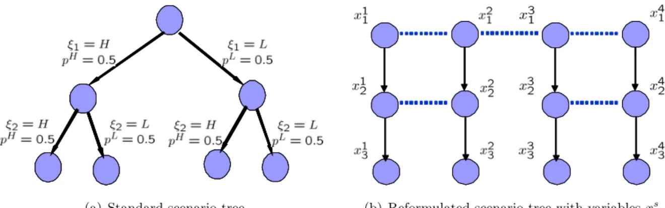
(a) Standard scenario tree (b) Reformulated scenario tree with variablesxst
Figure 1: Equivalent scenario trees
Section 7 presents theoretical properties that lead to reduction in the dimensionality of the model.
In section 8 we present a branch and bound algorithm based on Lagrangean duality to solve the proposed model. Finally, section 9 presents results to illustrate the advantages of our approach.
2 Background
We restrict the scope of this paper to problems where the uncertainty can be represented by discrete probability distributions and the time horizon is represented by a discrete set of time periods. For such problems, the stochastic process can be represented by a scenario tree, where each node represents a possible information state. An arc emanating from a node for time period t represents a possible transition to a node for time period t+ 1. The probability associated with an arc represents the probability of transition along that arc. Multiple arcs emanating from a node for time period trepresent multiple possibilities for transition and hence, that uncertainty in some parameter(s) will be resolved at the end of time period t. In a scenario tree, a path from the root node to a leaf node represents ascenario. Physically, a scenario represents one possible combination of values for all uncertain parameters. The probability of a scenario is the probability of reaching the corresponding leaf node from the root node.
Fig. 1(a) represents the scenario tree for a problem with two uncertain parametersξ1, ξ2 and three time periods. Possible realizations for both parameters includeH (“High”) and L (“Low”) where both realizations are equally probable. The uncertainties in ξ1 and ξ2 are resolved after the first and second time periods, respectively. The scenario tree has four scenarios, each with probability equal to 0.25.
Ruszczynski (1997) illustrates an alternative representation of scenario trees where each scenario is represented by a set of unique nodes (Fig. 1(b)). If the nodes for scenarios s, s0 in time period
t correspond to the same information state (represented by horizontal dotted lines linking the nodes in Fig. 1(b)), the two scenarios are said to be indistinguishable in time period t. In general, scenarioss, s0 are indistinguishable in time periodtif the two scenarios are identical in realizations for all uncertain parameters in which uncertainty has been resolved up till time t. The concept of indistinguishability is central to the non-anticipativity based approach to stochastic programming.
(SSP) is a “standard” stochastic program (Jonsbraten et al. (1998)) for a linear problem with T time periods and scenario treeS.
(SSP) min X
s
psX
t
cstxst (1a)
s.t. X
τ≤t
Asτ ,txsτ ≤ast ∀(t, s) (1b) xst ∈ Xts ∀(t, s) (1c) xst =xst0 ∀(s, s0, t)∈ NSe (1d) Parameterpsrepresents the probability of scenarioswhile variablesxst represent decision variables for time periodtin scenarios. (1a) represents the objective of minimizing the expectation of some economic criterion. Constraint (1b) represents single-period and period-linking constraints for a particular scenario which are characteristic of any multi-period model. Constraint (1c) represents integrality and bound restrictions on variablesxst. NSe represents the set of tuples (s, s0, t) such that scenariossand s0 are indistinguishable in time periodtfor scenario treeS. Thenon-anticipativity or implementability constraints (1d) link decisions for different scenarios. These constraints state that if scenarioss, s0 are indistinguishable in time periodtthen decisions fors, s0 intshould be the same. In other words, decisions cannot be based on knowledge that will be revealed in the future.
When the uncertainty is of exogenous nature, the probabilities ps and the set NSe are independent of the optimization variables. Thus, these are inputs to the optimization model. However, if the optimization decisions can influence the probability distribution, then probabilities ps have to be treated as optimization variables. On the other hand, if the optimization decisions influence the resolution of uncertainty, then the scenario tree and hence the set NSe depends on the decisions (Jonsbraten et al. (1998), Goel and Grossmann (2004)). We generalize the approach of Goel and Grossmann (2004) to problems with both exogenous and endogenous uncertainty by formulating the inter-dependence ofNSe and the optimization variables as a disjunctive program.
3 Motivating Example
The sizes problem (Jonsbraten et al. (1998), Jorjani et al. (1999)) is a specific example of the class of problems under consideration. In this problem, a production line has to meet the demand
for a product in a set of different sizes, I = {1,2, . . . , I}, in each time period of a time horizon T ={1,2, . . . , T}. If the demand for a size cannot be met, the deficit can be filled by the delivery of a bigger size. However, this involves a substitution cost. Other costs include fixed production costs for set-up of equipment for each size produced in each time period, variable inventory costs and variable production costs for each unit produced.
The demands, represented by ξt for time period t ∈ T, are uncertain. The variable costs of production, represented by θi for size i ∈ I, remain constant over the time horizon but are also uncertain. The demand in time periodtwill be observed automatically in that time period. On the other hand, the uncertainty in variable production cost for sizei,θi, will be resolved only when that size is produced for the first time. Thus, demand uncertainty is exogenous while the uncertainty in variable production costs is endogenous.
Decisions to be made in each time period include whether to produce sizeior not (binary variables bi,t), number of units of size ito be produced (variables yi,t) and number of units of size i to be used to satisfy demands of sizei0 (variablesxi,i0,t). Production decisions (bi,t, yt) are implemented at the beginning of time periodt. Then uncertainty is resolved in demands for time periodtand in variable production costs for sizes produced for the first time in time periodt. Finally, substitution decisions (xi,i0,t) are implemented to satisfy demands for time period t.
4 Generic problem description
In the class of problems under consideration, the time horizon is represented by the discrete set of time periods T = {1,2, . . . , T}. ξt represents the vector of exogenous uncertain parameters associated with time period t ∈ T. The uncertainty in ξt will be resolved automatically in time periodt. Ξ represents the discrete set of possible realizations for vectorξ = (ξ1, ξ2, . . . , ξT).
Set I ={1,2, . . . , I} represents the set of “sources” of endogenous uncertainty while θi represents the endogenous uncertain parameter associated with source i ∈ I. The discrete set of possible realizations for θi is represented by Θi. The resolution of uncertainty in θi depends on binary decision variablesbi,t. Specifically, the uncertainty inθi will be resolved in time period tif binary decisionbi,t= 1 andbi,τ = 0 ∀τ < t. Besides decisions represented by variablesbi,t, other decisions to be made in time periodt are represented by variables yt andxttogether.
The sequence of events in each time period is as follows. Decisions yt and bi,t are implemented at the beginning of time period t. This is followed by resolution of uncertainty in the exogenous parameters ξt and in the endogenous parameter θi for source i if bi,t = 1 and bi,τ = 0 ∀τ < t.
Finally, decisionsxt are implemented at the end of the time period.
In general, variables bi,t may represent investment or operation decisions associated with source i.
In the sizes problem, variables bi,t represent whether sizeiis produced in time period tor not. In the gas field problem considered by Goel and Grossmann (2004), these variables represent whether or not investment is made at field i in time period t. The uncertainty associated with a size or a field is resolved in time period tif the production of that size or the investment at that field is carried out for the first time in time period t.
Note that for ease of exposition, we assume that there is only one endogenous uncertain parameter associated with source i for all i ∈ I. Thus, we assume that θi is a scalar for all i ∈ I. At the end of section 7 we describe how our approach extends to the more general case where θi may be a vector for some i∈ I.
5 Notations and definitions
In order to make the following discussion more comprehensible, we first explain the notation and definitions used in this paper. Each scenario in this problem corresponds to one possible realization for the vector (ξ1, ξ2, . . . , ξT, θ1, θ2, . . . , θI). We assume that the set of scenarios corresponds to Ξ×(×i∈IΘi), i.e., for any realization of the vector of exogenous parameters,ξ = (ξ1, ξ2, . . . , ξT), the set of scenarios includes scenarios corresponding to all possible combinations of realizations for the endogenous parameters. Individual scenarios are indexed as s ∈ S, where S = {1,2, . . . , S}
represents the set of indices corresponding to all the scenarios. Note that we will use index s to refer to the corresponding scenario. Further, θsi and ξst will represent the realizations of θi and ξt respectively, in scenario s.
For scenarios s, s0 ∈ S, the set D(s, s0) = {i|i ∈ I, θsi 6= θsi0} represents the set of sources of endogenous uncertainty that distinguish scenarios sand s0. |D(s, s0)|represents the cardinality of this set. In general, 0 ≤ |D(s, s0)| ≤ I holds for all s, s0 ∈ S, where I is the number of sources of endogenous uncertainty. By definition,D(s, s0) =D(s0, s).
For scenarios s, s0 ∈ S, t(s, s0) is the latest time period t such that realizations of all exogenous parameters resolved up till and includingtare the same in scenarioss, s0. In other words,t(s, s0) is the last time period at the end of which scenariossands0 are indistinguishable based on exogenous uncertainty resolved. Mathematically,
t(s, s0) = max
t {t|t∈ T, ξsτ =ξsτ0 ∀τ ∈ T, τ ≤t}
If {t|t ∈ T, ξsτ = ξsτ0 ∀τ ∈ T, τ ≤ t} = ∅ , then we define t(s, s0) = 0. Note that there cannot be distinct scenarioss, s0 ∈ S such that|D(s, s0)|= 0 andt(s, s0) =T. This is because if s, s0 satisfied the above conditions then they would be completely identical. By definition, t(s, s0) =t(s0, s).
L0 = {(s, s0)|s, s0 ∈ S, s < s0,|D(s, s0)| = 0} represents the set of scenario pairs (s, s0) such that scenariossands0 are identical in terms of realizations for all endogenous parameters. The condition s < s0 prevents duplicate entries in L0 for the same pair of scenarios s, s0.
L1+ ={(s, s0)|s, s0 ∈ S, s < s0,|D(s, s0)| ≥1}represents the set of scenario pairs (s, s0) such thats, s0 differ in realizations of θi for at least one i∈ I. Also, L1 ={(s, s0)|s, s0 ∈ S, s < s0,|D(s, s0)|= 1}.
L1T = {(s, s0)|(s, s0) ∈ L1,t(s, s0) = T} is the set of scenario pairs (s, s0) such that scenarios s, s0 differ in the realization of only one endogenous parameter and are identical in realizations for all exogenous parameters.
6 Model
In this section we introduceP1, the declarative form of stochastic programs for the class of problems described in section 4.
(P1) φ= min X
s∈S
psX
t∈T
Ã
wcstwts+xcstxst +ycstyts+X
i∈I
bcsi,tbsi,t
!
(2)
s.t. X
τ∈T, τ≤t
Ã
wAsτ ,twτs+xAsτ ,txsτ+yAsτ ,tyτs+X
i∈I
bAsi,τ ,tbsi,τ
!
≤ast ∀s∈ S, t∈ T (3)
bsi,1 =bsi,10 ∀s, s0 ∈ S, s < s0, i∈ I (4a) y1s =y1s0 ∀s, s0 ∈ S, s < s0 (4b) xst =xst0 ∀(s, s0)∈ L0, t∈ T, t≤t(s, s0) (5a) bsi,t+1 =bsi,t+10 ∀(s, s0)∈ L0, t∈ T, t≤t(s, s0), i∈ I (5b) yt+1s =yt+1s0 ∀(s, s0)∈ L0, t∈ T, t≤t(s, s0) (5c)
Zts,s0 xst = xst0
bsi,t+1 = bsi,t+10 ∀i∈ I ift≤T −1 yt+1s = yst+10 ift≤T −1
∨h
¬Zts,s0i
∀(s, s0)∈ L1+, t∈ T, t≤t(s, s0) (6)
Zts,s0 ⇔ ^
i∈D(s,s0)
" t
^
τ=1
¡¬bsi,τ¢
#
∀(s, s0)∈ L1+, t∈ T, t≤t(s, s0) (7)
Zts,s0 ⇔ ^
i∈D(s,s0)
" t
^
τ=1
³¬bsi,τ0 ´
#
∀(s, s0)∈ L1+, t∈ T, t≤t(s, s0) (8)
wts∈ Wts, xst ∈ Xts, yts∈ Yts, bsi,t ∈ {0,1} ∀s∈ S, t∈ T, i∈ I
Zts,s0 ∈ {T rue, F alse} ∀(s, s0)∈ L1+, t∈ T, t≤t(s, s0)
In P1, variables bsi,t, xst and yts represent the decisions to be made in time period t of scenario s.
Vector wts represents the other variables associated with time period t in scenario s. In process control terminology, bsi,t, xst and yst are “control variables” whilewts are “state variables”. bsi,t are binary variables while xst and yts are variable vectors that may have both integer and continuous components. As explained in section 4, decisions yts and bsi,t are implemented at the beginning of time periodt, while decisionsxst are implemented at the end of the time period after the resolution of uncertainty in that time period.
The realizations of the cost coefficients of variablesb(·)i,t,x(·)t ,yt(·)andw(·)t in scenariosare represented by bcsi,t, xcst, ycst and wcst, respectively. Similarly, bAsi,τ ,t, xAsτ ,t, yAsτ ,t and wAsτ ,t represent the realizations of the constraint coefficient matrices (or vectors) of these variables in scenario s. (2) represents the objective of minimizing the expectation of an economic criterion. (3) represents single-period and period-linking constraints for a particular scenario. These include the square system of equality constraints which can be used to eliminate “state” variableswts.
Decisions for different scenarios are linked by non-anticipativity constraints, (4)-(8). The non- anticipativity rule requires that if scenarios s and s0 are indistinguishable at some time, then decisions in scenarios sand s0 should be the same at that time. Based on the sequence of events described in section 4, uncertainty is resolved in time periodtafter the implementation of decisions yts and bsi,t. Thus, if scenarios s, s0 are indistinguishable after resolution of uncertainty in time periodt, then decisions x(·)t ,b(·)i,t+1 andyt+1(·) should be the same for scenarioss, s0. Note that in this paper, we refer to the “indistinguishability of the two scenarios after the resolution of exogenous and endogenous uncertainty in time periodt” simply by the “indistinguishability of two scenarios in time periodt”.
Based on the sequence of events in each time period, all scenarios are indistinguishable before decisions bsi,t and yts are implemented in the first time period. Thus, decisionsb(·)i,1 and y(·)1 have to be the same for all scenarios (4). Note that the conditions < s0 is imposed to avoid duplication of constraints (4) for the same pair of scenarios s, s0.
(5) represents non-anticipativity constraints linking scenarios s, s0 such that (s, s0) ∈ L0; i.e., the realizations of all endogenous parameters in scenarios s and s0 are identical. In this case, scenarioss, s0 will be indistinguishable in time periodtif and only if these scenarios are identical in realizations of all exogenous parameters observed up till and including time period t. Accordingly, (5) applies non-anticipativity constraints on decisions x(·)t , y(·)t+1, b(·)i,t+1 for scenarios s, s0 only if t satisfiest≤t(s, s0).
(6)-(8) are non-anticipativity constraints linking scenarios s, s0 such that (s, s0) ∈ L1+; i.e., sce-
narios s and s0 differ in the realization of at least one endogenous parameter. In this case, the indistinguishability of scenarios s, s0 in time period t depends on both, endogenous and exoge- nous uncertainty resolved in the past. Boolean variable Zts,s0 is T rue if and only if scenarios s and s0 are indistinguishable (after the resolution of uncertainty) in time period t. Clearly, for t > t(s, s0) scenarios s, s0 can be distinguished simply based on realizations of the exogenous pa- rameters. Hence,Zts,s0 =F alse fort >t(s, s0). Therefore constraints (6)-(8) are applied only fort such that t≤t(s, s0), where (s, s0)∈ L1+.
Disjunction (6) imposes the non-anticipativity constraints on variablesx(·)t , yt+1(·) , b(·)i,t+1 for scenarios s, s0 only if Zts,s0 is T rue, i.e., if scenarios s and s0 are indistinguishable in time period t. By definition of t(s, s0), if t ≤ t(s, s0) then the indistinguishability of scenarios s, s0 in time period t depends purely on the endogenous uncertainty resolved through the decisions. Logic constraints (7) and (8) relate the indistinguishability of scenarios s, s0 in time period t with decisions bsi,τ and bsi,τ0 respectively. Scenarios s, s0 differ in realizations of a finite set of endogenous parameters.
Constraint (7) states1 thatZts,s0 is T rueif and only if uncertainty has not been resolved in any of these parameters up till (and including) time period tof scenarios. Similarly, (8) relates variables Zts,s0 to the corresponding decision variables for scenarios0.
Note that to account for the offset in the time index of these variables, the non-anticipativity constraints on variablesb(·)i,t+1, yt+1(·) for scenarioss, s0 are applied only ift≤T−1. Although it may seem that a similar restriction is needed in (5b)-(5c), however, as explained earlier in this section, we cannot have distinct scenarios s, s0 ∈ S such that (s, s0) ∈ L0 and t(s, s0) = T. Hence, the condition thatt≤T −1 is implicit in the conditiont≤t(s, s0) in (5b)-(5c).
Wts,Xtsand Yts represent the bounds and integrality restrictions on variableswst,xst andyts respec- tively, for allt∈ T, s∈ S.
7 Model properties
In this section, we present a set of properties that lead to reduction in the dimensionality of the proposed model. Note that we will use bs to represent the vector of variables bsi,t for all (i, t).
Similarly, vector b will represent the vector of bs for all s. The same convention will be used to represent vectors of variables wts, xst, yts, Zts,s0 and parameters introduced later in the paper.
The tuple (b, w, x, y, Z) will be used to represent a solution to the model under consideration.
Further, in all properties presented in this paper, it is assumed that variables bsi,t ∈ {0,1} and
1In theory, the logical operator “¬” should only be used with Boolean variables. Sincebsi,tare binary variables, therefore constraints (7) and (8) involve a slight inconsistency in notation. A more rigorous formulation can be obtained at the expense of additional notation by defining (7) and (8) in terms of Boolean variablesBi,ts and specifying an equivalence between variablesBsi,tandbsi,t.
Zts,s0 ∈ {T rue, F alse}. Similarly, solutions ˆbsi,t ∈ {0,1}and ˆZts,s0 ∈ {T rue, F alse}.
Proposition 1. Consider constraints (9)-(11) for given s, s0,ˆt where s, s0∈ S,tˆ∈ T,ˆt≤T −1.
bsi,1 =bsi,10 ∀i∈ I (9)
"
Zts,s0
bsi,t+1 = bsi,t+10 ∀i∈ I
#
∨h
¬Zts,s0i
∀t∈ T, t≤ˆt (10)
Zts,s0 ⇔ ^
i∈D(s,s0)
" t
^
τ=1
¡¬bsi,τ¢
#
∀t∈ T, t≤ˆt (11) If vectors ˆbs,ˆbs0,Zˆs,s0 satisfy (9)-(11) then,
(a) For t∈ T, t≤ˆt,
^
i∈D(s,s0)
" t
^
τ=1
³
¬ˆbsi,τ´
#
⇒h
ˆbsi,τ = ˆbsi,τ0 ∀i∈ I, τ ∈ T, τ ≤t+ 1i
(b) For t= ˆt+ 1,
^
i∈D(s,s0)
" t
^
τ=1
³
¬ˆbsi,τ´
#
⇒h
ˆbsi,τ = ˆbsi,τ0 ∀i∈ I, τ ∈ T, τ ≤ti
(c) For t∈ T, t≤ˆt+ 1,
^
i∈D(s,s0)
" t
^
τ=1
³¬ˆbsi,τ´
#
⇔ ^
i∈D(s,s0)
" t
^
τ=1
³¬ˆbsi,τ0 ´
#
(d) For t∈ T, t≤ˆt,
^
i∈D(s,s0)
" t
^
τ=1
³¬ˆbsi,τ0 ´
#
⇒h
ˆbsi,τ = ˆbsi,τ0 ∀i∈ I, τ ∈ T, τ ≤t+ 1.i
(e) For t= ˆt+ 1,
^
i∈D(s,s0)
" t
^
τ=1
³¬ˆbsi,τ0 ´
#
⇒h
ˆbsi,τ = ˆbsi,τ0 ∀i∈ I, τ ∈ T, τ ≤t.i
Note that the left hand sides of (a) and (b) involve variablesbsi,τ while the left hand sides of (d) and (e) involve variables bsi,τ0 .
Proof. See Appendix A.
We use Proposition 1 as a basis to prove the following theorem.
Theorem 1. If solution (ˆb,w,ˆ x,ˆ y,ˆ Zˆ) satisfies (4a), (6) and (7), then it also satisfies (8). Thus, constraint (8) is redundant in P1.
Proof. Suppose solution (ˆb,w,ˆ x,ˆ y,ˆ Zˆ) satisfies (4a), (6) and (7). Consider scenariossa, sb ∈ S such that (sa, sb)∈ L1+. We will prove that solution (ˆb,w,ˆ x,ˆ y,ˆ Z) satisfies (8) for (s, sˆ 0) = (sa, sb). The theorem follows as a result.
By definition, t(sa, sb) = max
t {t|t ∈ T, ξsτa = ξsτb ∀τ ∈ T, τ ≤ t}. If {t|t ∈ T, ξsτa = ξsτb ∀τ ∈ T, τ ≤ t} = ∅, then by convention t(sa, sb) = 0. Hence, (ˆb,w,ˆ x,ˆ y,ˆ Z) satisfies (8) vacuously forˆ (s, s0) = (sa, sb).
If {t|t∈ T, ξsτa =ξsτb ∀τ ∈ T, τ ≤t} 6=∅, then t(sa, sb)≥1. Since (ˆb,w,ˆ x,ˆ y,ˆ Zˆ) satisfies (4a), (6) and (7) and (sa, sb)∈ L1+, therefore sub-vectors ˆbsa,ˆbsb,Zˆsa,sb satisfy (9)-(11) for (s, s0) = (sa, sb), ˆt = min(T −1,t(sa, sb)). (The equality constraint on variablesb(·)i,t+1 inside (6) is applied only if t≤T−1. Hence, (ˆbsa,ˆbsb,Zˆsa,sb) is guaranteed to satisfy (10) only fort≤min(T−1,t(sa, sb))).
Using result (c) of Proposition 1, we get
^
i∈D(sa,sb)
" t
^
τ=1
³¬ˆbsi,τa´
#
⇔ ^
i∈D(sa,sb)
" t
^
τ=1
³¬ˆbsi,τb´
#
∀t∈ T, t≤min(T −1,t(sa, sb)) + 1
Since t(sa, sb)≤T, therefore min(T −1,t(sa, sb)) + 1 = min(T,t(sa, sb) + 1)≥t(sa, sb). Hence,
^
i∈D(sa,sb)
" t
^
τ=1
³¬ˆbsi,τa´
#
⇔ ^
i∈D(sa,sb)
" t
^
τ=1
³¬ˆbsi,τb´
#
∀t∈ T, t≤t(sa, sb) (12)
Since sub-vectors ˆbsa,ˆbsb,Zˆsa,sb satisfy (7) for (s, s0) = (sa, sb), we can combine (7) with (12) to infer that sub-vectors ˆbsa,ˆbsb,Zˆsa,sb satisfy (8). The result follows.
Proposition 2. Consider constraints (13)-(16)in variables b, x, y, Z defined over the tuple(s, s0, t)
bsi,t = bsi,t0 ∀i∈ I (13a)
yst = yst0 (13b)
xst = xst0 (14a)
bsi,t+1 = bsi,t+10 ∀i∈ I (14b)
yst+1 = yst+10 (14c)
Zts,s0 xst = xst0
bsi,t+1 = bsi,t+10 ∀i∈ I if t≤T −1 yt+1s = yst+10 if t≤T −1
∨h
¬Zts,s0i
(15)
Zts,s0 ⇔ ^
i∈D(s,s0)
" t
^
τ=1
¡¬bsi,τ¢
#
(16)
If vectors ˆb,x,ˆ y,ˆ Zˆ satisfy
(i) Constraints (13a)-(13b) for(s, s0, t) such thats, s0 ∈ S, s < s0, t= 1 (ii) Constraint (14) for (s, s0, t) such that (s, s0)∈ L0, t∈ T, t≤t(s, s0) (iii) Constraints (15)-(16) for (s, s0, t) such that(s, s0)∈ L1T, t∈ T
thenˆb,x,ˆ y,ˆ Zˆ satisfy constraints (15)-(16) for (s, s0, t) such that (s, s0)∈ L1+, t∈ T, t≤t(s, s0).
Proof. See Appendix C (Based on Lemma 1, Appendix B).
Based on the above proposition, we define modelP2 where (17) and (18) are applied instead of (6) and (7), respectively. Also, (8) has been dropped.
(P2) φ= min X
s∈S
psX
t∈T
Ã
wcstwst+xcstxst+ycstyts+X
i∈I
bcsi,tbsi,t
!
s.t. (3),(4),(5)
Zts,s0 xst = xst0
bsi,t+1 = bsi,t+10 ∀i∈ I ift≤T −1 yt+1s = yst+10 ift≤T −1
∨h
¬Zts,s0i
∀(s, s0)∈ L1T, t∈ T (17) Zts,s0 ⇔
" t
^
τ=1
¡¬bsi,τ¢
#
∀(s, s0)∈ L1T, t∈ T,{i}=D(s, s0) (18) wst ∈ Wts, xst ∈ Xts, yts∈ Yts, bsi,t ∈ {0,1} ∀s∈ S, t∈ T, i∈ I
Zts,s0 ∈ {T rue, F alse} ∀(s, s0)∈ L1T, t∈ T
Theorem 2. If (ˆb,w,ˆ x,ˆ y,ˆ Z)ˆ is an optimal solution P1 then it is also an optimal solution of P2, and vice versa.
Proof. Since the objective functions of P1 and P2 are the same, it is sufficient to show that the feasible regions ofP1 andP2 are the same.
Suppose (ˆb,w,ˆ x,ˆ y,ˆ Z) is a feasible solution ofˆ P1. Compare modelsP1 andP2. Constraints (3)-(5) are common to both models while disjunctions (17) and (6) differ only in the domain for (s, s0, t).
Constraint (18) differs from (7) in the domain for (s, s0, t) and in the right hand side of the logic relationship.
LetF1denote the domain of (s, s0, t) in (6)-(7) and letF2denote the domain of (s, s0, t) in (17)-(18).
Thus,
F1 ={(s, s0, t)|(s, s0)∈ L1+, t∈ T, t≤t(s, s0)}
F2 ={(s, s0, t)|(s, s0)∈ L1T, t∈ T }.
where,
L1T ={(s, s0)|(s, s0)∈ L1,t(s, s0) =T} By definition,
L1T ⊆ L1 ⊆ L1+. Now,
F2 = {(s, s0, t)|(s, s0)∈ L1T, t∈ T }
≡ {(s, s0, t)|(s, s0)∈ L1T, t∈ T, t≤t(s, s0)} (sincet(s, s0) =T for (s, s0)∈ L1T)
⊆ {(s, s0, t)|(s, s0)∈ L1+, t∈ T, t≤t(s, s0)} (sinceL1T ⊆ L1+)
= F1
Also, |D(s, s0)| = 1 for (s, s0, t) ∈ F2. Therefore, the right hand side of (7) reduces to the right hand side of (18). SinceF2⊆ F1, therefore P2 is a relaxation of P1. Thus (ˆb,w,ˆ x,ˆ y,ˆ Z) should beˆ a feasible solution ofP2.
Conversely, suppose (ˆb,w,ˆ x,ˆ y,ˆ Z) is a feasible solution ofˆ P2. Thus, (ˆb,w,ˆ x,ˆ y,ˆ Zˆ) satisfies (3), (4), (5), (17) and (18). Using Proposition 2 we can infer that (ˆb,w,ˆ x,ˆ y,ˆ Zˆ) satisfies (6) and (7).
Further, using Theorem 1 we can infer that (ˆb,w,ˆ x,ˆ y,ˆ Z) satisfies (8). Thus, (ˆˆ b,w,ˆ x,ˆ y,ˆ Z) is aˆ feasible solution of P1.
The following remarks can be made about the proposed model.
1. According to model P2, non-anticipativity constraints need to be applied for scenarios s and s0 only if the scenarios either differ exclusively in realizations for exogenous uncertain parameters, or differ exclusively in the realization of one endogenous uncertain parameter.
2. The “standard” stochastic programming formulation (1) is clearly a specific case of modelP2 when there is only exogenous uncertainty (L1+ =L1T =∅).
3. The proofs of Proposition 1, Theorem 1 and Theorem 2 are independent of the choice of the set of scenarios. To illustrate the dependence of Proposition 2 on the set of scenarios, consider indices sa, sb ∈ S such that the corresponding scenarios differ in the realizations of r endogenous parameters, where r = |D(sa, sb)| ≥ 1. Broadly, Proposition 2, which is used in Theorem 2, is based on the assumption that there exist indices s1, s2, . . . , sr ∈ S such that (sa, s1),(s1, s2),(s2, s3), . . . ,(sr−1, sr) ∈ L1T while (sr, sb) ∈ L0. Proposition 2 is then a result of the fact that the non-anticipativity constraints linkingsa withsb are implied by the
“chaining” of non-anticipativity constraints linking sa with s1, s1 with s2, s2 with s3, . . ., sr−1 with sr andsr with sb.
Since we choose the set of scenarios as Ξ×(×i∈IΘi), for any realization of the vector of exogenous parametersξ, the set of scenarios includes all possible combinations of realizations for the endogenous parameters. Thus, we can generate r “intermediate” scenarios from sce- nario sa by progressively changing the realization of one of ther distinguishing endogenous parameters to the corresponding realization in scenario sb. The realizations of all exogenous parameters in these r scenarios are identical to those in sa. Since sa ∈ S, these r scenar- ios also belong to the set of scenarios. Thus, we can choose indices s1, s2, . . . , sr ∈ S for these rscenarios. Hence, the non-anticipativity constraints for sa, sb follow by “chaining”, as explained above.
4. The models and proofs presented here are based on the assumption that the endogenous uncertainty associated with source i can be represented by one parameter. Thus, θi is a scalar. To consider the more general case, suppose θi is an ni×1 vector. For example, in the gas field problem, the uncertainty in a field is represented by uncertainty in the size and quality of the field. Therefore, in that problem ni= 2 for each fieldi.
If we choose the set of scenarios as Ξ ×(×i∈IΘi), where (×i∈IΘi) represents all possible combinations of realizations for vectors θi for all i, then we can again use the “chaining”
argument to prove that the solutions to models P1 and P2 are the same for L1T ={(s, s0)| s, s0∈ S, s < s0,t(s, s0) =T,
∃(i∗, l∗), i∗ ∈ I, l∗∈ {1,2, . . . , ni∗} such that θsl∗,i∗ 6=θsl∗0,i∗,
θsl,i=θsl,i0 ∀l∈ {1,2, . . . , ni}, i∈ I \ {i∗}}
However, stronger results may be obtained if the set of scenarios is chosen as Ξס
×i∈I
¡×nl=1i Θl,i
¢¢, where Θl,i represents the set of possible realizations for endogenous uncertain parameter θl,i associated with source i. The “chaining” argument can then be used to prove that the solu- tions to modelsP1 and P2 are the same for
L1T ={(s, s0)| s, s0∈ S, s < s0,t(s, s0) =T,
∃(i∗, l∗), i∗ ∈ I, l∗∈ {1,2, . . . , ni∗} such that θsl∗,i∗ 6=θsl∗0,i∗,
θsl,i∗ =θsl,i0∗ ∀l∈ {1,2, . . . , ni∗} \ {l∗}, θsl,i=θsl,i0 ∀l∈ {1,2, . . . , ni}, i∈ I \ {i∗}}
In other words, the disjunctive non-anticipativity constraints will need to be applied between scenarios s, s0 only if the two scenarios differ in the realization of exactly one endogenous scalar parameter,θl∗,i∗ for some source i∗ ∈ I.
5. In the present form, P2 has disjunctions and linear constraints linking Boolean, binary and continuous variables. The model can be reformulated as a mixed integer linear program by representing Boolean variables Zts,s0 as 0-1 variables zs,st 0 and reformulating the logic con- straints and disjunctions as linear constraints using big-M or convex hull reformulations (Balas (1985), Turkay and Grossmann (1996)). It should be noted that if (18) is reformulated as linear constraints, then variables zs,st 0 will satisfy the integrality condition even if they are represented by continuous variables with bounds 0≤zts,s0 ≤1.
However, solving the MILP reformulation of P2 may be an inefficient approach for large problems. In the next section, we present a specialized branch and bound algorithm motivated by the work of Caroe and Schultz (1999).
8 Branch and bound algorithm
Model P2 is coupled in scenarios through the non-anticipativity constraints. In the proposed branch and bound algorithm, lower bounds at each node are generated by solving a Lagrangean dual problem which is obtained by relaxing the non-anticipativity constraints. Each sub-problem in the Lagrangean dual problem corresponds to an MILP for one of the scenarios. An outline of the proposed algorithm is presented in Fig. 2. P denotes the list of current problems together with the associated lower bounds, φRLD, while φU B represents the objective value of the best feasible solution obtained. The steps of the algorithm are explained in more detail below. For simplicity, we assume that all integer components of variables xst and yts correspond to binary variables.