Time-Varying Uncertainty and the Credit Channel

IHS Economics Series Working Paper 118

July 2002

Time-Varying Uncertainty and the Credit Channel

Victor Dorofeenko

Gabriel S. Lee

Kevin D. Salyer

Impressum Author(s):

Victor Dorofeenko, Gabriel S. Lee, Kevin D. Salyer Title:

Time-Varying Uncertainty and the Credit Channel ISSN: Unspecified

2002 Institut für Höhere Studien - Institute for Advanced Studies (IHS) Josefstädter Straße 39, A-1080 Wien

E-Mail: o ce@ihs.ac.atffi Web: ww w .ihs.ac. a t

All IHS Working Papers are available online: http://irihs. ihs. ac.at/view/ihs_series/

This paper is available for download without charge at:

https://irihs.ihs.ac.at/id/eprint/1441/

Time-Varying Uncertainty and the Credit Channel

Victor Dorofeenko, Gabriel S. Lee, Kevin D. Salyer

118

Reihe Ökonomie

Economics Series

118 Reihe Ökonomie Economics Series

Time-Varying Uncertainty and the Credit Channel

Victor Dorofeenko, Gabrie l S. Lee, Kevin D. Salyer July 2002

Institut für Höhere Studien (IHS), Wien

Institute for Advanced Studies, Vienna

Contact:

Victor Dorofeenko

Department of Economics and Finance Institute for Advanced Studies

Stumpergasse 56, A-1060 Vienna, Austria (: +43/1/599 91-183

fax: +43/1/599-91-163 email: dorofeen@ihs.ac.at

Gabriel S. Lee

Department of Economics and Finance Institute for Advanced Studies

Stumpergasse 56, A-1060 Vienna, Austria (: +43/1/599 91-141

fax: +43/1/599-91-163 email: lee@ihs.ac.at

Kevin D. Salyer

Department of Economics University of California Davis, CA 95616, USA (: +1/530/752-8359 email: kdsalyer@ucdavis.edu

Founded in 1963 by two prominent Austrians living in exile – the sociologist Paul F. Lazarsfeld and the economist Oskar Morgenstern – with the financial support from the Ford Foundation, the Austrian Federal Ministry of Education and the City of Vienna, the Institute for Advanced Studies (IHS) is the first institution for postgraduate education and research in economics and the social sciences in Austria.

The Economics Series presents research done at the Department of Economics and Finance and aims to share “work in progress” in a timely way before formal publication. As usual, authors bear full responsibility for the content of their contributions.

Das Institut für Höhere Studien (IHS) wurde im Jahr 1963 von zwei prominenten Exilösterreichern – dem Soziologen Paul F. Lazarsfeld und dem Ökonomen Oskar Morgenstern – mit Hilfe der Ford- Stiftung, des Österreichischen Bundesministeriums für Unterricht und der Stadt Wien gegründet und ist somit die erste nachuniversitäre Lehr- und Forschungsstätte für die Sozial- und Wirtschafts - wissenschaften in Österreich. Die Reihe Ökonomie bietet Einblick in die Forschungs arbeit der Abteilung für Ökonomie und Finanzwirtschaft und verfolgt das Ziel, abteilungsinterne Diskussionsbeiträge einer breiteren fachinternen Öffentlichkeit zugänglich zu machen. Die inhaltliche Verantwortung für die veröffentlichten Beiträge liegt bei den Autoren und Autorinnen.

Abstract

We extend the Carlstrom and Fuerst (1997) agency cost model of business cycles by including time varying uncertainty in the technology shocks that affect capital production. We first demonstrate that standard linearization methods can be used to solve the model yet second moment effects still influence equilibrium characteristics. The effects of the persistence of uncertainty are then analyzed. Our primary findings fall into three broad categories. First, it is demonstrated that uncertainty affects the level of the steady-state of the economy so that welfare analyses of uncertainty that focus entirely on the variability of output (consumption) will understate the true costs of uncertainty. A second key result is that time varying uncertainty results in countercyclical bankruptcy rates – a finding which is consistent with the data and opposite the result in Carlstrom and Fuerst. Third, we show that persistence of uncertainty affects both quantitatively and qualitatively the behavior of the economy.

Keywords

Agency costs, credit channel, time-varying uncertainty

JEL Classifications

E2, E4, E5

Comments

We wish to thank the participants in the UC Davis Macroeconomic Seminar and CEF 2002 in Aix en Provence for helpful comments and suggestions.

Contents

1 Introduction 1

2 Model 3

2.1 Households ...4

2.2 Firms...5

2.3 Entrepreneurs ...6

2.4 Optimal Financial Contract...6

2.5 Entrepreneur’s Consumption Choice...9

2.6 Financial Intermediaries ... 11

2.7 Equilibrium ... 11

3 Equilibrium Characteristics 12

3.2 Cyclical Behavior... 16

Figures 20 4 Conclusion 23 References 24 5 Appendix: Steady-state conditions in the Carlstrom and Fuerst Agency Cost Model 25

5.1 Definition of Steady -state ... 28

1 Introduction

Business cycle research has long associated risk with cyclical movements in the economy.

It is therefore somewhat surprising that modern macroeconomics has, until quite recently, ignored the interaction between uncertainty and cyclical dynamics. This lack of study did not, however, reflect an inherent lack of interest, but was instead driven by primarily technological constraints: the typical solution method used in solving calibrated business cycle models imposes certainty equivalence so that the influence of uncertainty (i.e. second moment effects) are ruled out by construction.

One of the first models in which the variance of shocks played a prominent role was that developed by Obstfeld and Rogoff (2000). While this analysis provided important insights into the effects of uncertainty (identified with the variance of money growth and productivity shocks), the setting abstracted from capital accumulation so that the impact of risk on investment could not be studied. Only very recently, have solution methods for quantitative macroeconomic models (i.e. models in which the parameters can be calibrated to key features of the economy) been developed that do not impose certainty equivalence. In particular, Collard and Juillard (forthcoming), Sims (2001) and Grohe-Schmitt and Uribe (2001) present different solution techniques in which the second moments influence equilibrium dynamics.

The analysis presented here continues the emphasis on second moments but departs

from previous work by conducting the analysis within a setting in which information and

uncertainty play prominent roles in equilibrium characteristics. Specifically, we use the

business cycle model developed by Carlstrom and Fuerst (1997). This model is particularly

attractive for our purposes since it incorporates a lending channel (for investment) that is characterized by asymmetric information between lenders and borrowers. In addition, this model is a variant of a typical real business cycle model so that key parameters can be calibrated to the data. Within this setting, we model time varying uncertainty as a mean preserving spread in the distribution of the technology shocks affecting capital production and explore how changes in uncertainty affect equilibrium characteristics.

We first demonstrate that linearization solution methods can be employed yet this does

not eliminate the effects of second moments. That is, in solving for the linear equilibrium policy functions, the vector of state variables includes the variance of technology shocks buffeting the capital production sector. We then examine how the persistence of a change in the variance influences equilibrium characteristics. One of the primary findings is that time varying uncertainty produces countercyclical bankruptcy rates. In contrast, Carlstrom and Fuerst’s (1997) analysis of aggregate technology shocks produced the counterfactual prediction of procyclical bankruptcy rates. Hence, the analysis presented here demonstrates that second moment effects, not surprisingly, expand the set of equilibrium characteristics;

moreover, in some instances, first and second moment effects move in opposite directions.

This may have important consequences for understanding historical business cycles. That

is, historical business cycles can be differentiated by whether the shocks are predominantly to

aggregate supply or aggregate demand. Our analysis suggests that another useful distinction

may be the role of information; namely, is it the first or second moments of the shocks hitting

the economy that is dominant in influencing equilibrium characteristics.

The next section presents the model while the following section discusses equilibrium characteristics. The final section offers some concluding comments.

2 Model

We employ the agency cost business cycle model of Carlstrom and Fuerst (1997) to address the financial intermediaries’ role in the propagation of productivity shocks and extend their analysis by introducing time-varying uncertainty. Since, for the most part, the model is identical to that in Carlstrom and Fuerst, the exposition of the model will be brief.

The model is a variant of a standard RBC model in which an additional production sector is added. This sector produces capital using a technology which transforms investment into capital. In a standard RBC framework, this conversion is always one-to-one; in the Carlstrom and Fuerst framework, the production technology is subject to technology shocks.

(The aggregate production technology is also subject to technology shocks as is standard.)

This capital production sector is owned by entrepreneurs who finance their production via

loans from a risk neutral financial intermediation sector - this lending channel is characterized

by a loan contract with a fixed interest rate. (Both capital production and the loans are

intra-period.) If a capital producing firm realizes a low technology shock, it will declare

bankruptcy and the financial intermediary will take over production; this activity is subject

to monitoring costs. With this brief description, we now turn to an explicit characterization

of the economy.

2.1 Households

The representative household is infinitely lived and has expected utility over consumption c

and leisure 1 − l

with functional form given by:

E

P

β

[ln (c

) + ν (1 − l

)] (1) where E

denotes the conditional expectation operator on time zero information, β ∈ (0, 1) , ν > 0, and l

is time t labor. The household supplies labor, l

, and rents its accumulated capital stock, k

, to firms at the market clearing real wage, w

, and rental rate r

, respectively, thus earning a total income of w

l

+ r

k

. The household then purchases consumption good

from firms at price of one (i.e. consumption is the numeraire), and purchases new capital,

i

, at a price of q

. Consequently, his budget constraint is

w

l

+ r

k

≥ c

+ q

i

(2) The law of motion for households’ capital stock is standard:

k

= (1 − δ) k

+ i

(3)

where δ ∈ (0, 1) is the depreciation rate on capital.

The necessary conditions associated with the maximization problem include the standard labor-leisure condition and the intertemporal efficiency condition associated with investment.

Given the functional form for preferences, these are:

νc

= w

(4)

q

c

= βE

· q

(1 − δ) + r

c

¸

(5)

2.2 Firms

The economy’s output of the consumption good is produced by firms using Cobb-Douglas technology

Y

= θ

K

H

(H

)

(6) where Y

represents the aggregate output, θ

denotes the aggregate technology shock, K

denotes the aggregate capital stock, H

denotes the aggregate household labor supply, H

denotes the aggregate supply of entrepreneurial labor, and α

+ α

+ α

= 1.

The profit maximizing representative firm’s first order conditions are given by the fac- tor market’s condition that wage and rental rates are equal to their respective marginal productivities:

w

= θ

α

Y

H

(7) r

= θ

α

Y

K

(8) w

= θ

α

Y

H

(9)

where w

denotes the wage rate for entrepreneurial labor.

1 Note that we denote aggregate variables with upper case while lower case represents per-capita values.

Prices are also lower case.

2 As in Carlstrom and Fuerst, we assume that the entrepreneur’s labor share is small, in particular, α_H^e = 0.0001. The inclusion of entrepreneurs’ labor into the aggregate production function serves as a technical device so that entrepreneurs’ net worth is always positive, even when insolvent.

2.3 Entrepreneurs

A risk neutral representative entrepreneur’s course of action is as follows. To finance his project at period t, he borrows resources from the Capital Mutual Fund according to an optimal financial contract. The entire borrowed resources, along with his total net worth at period t, are then invested into his capital creation project. If the representative entrepreneur is solvent after observing his own technology shock, he then makes his consumption decision;

otherwise, he declares bankruptcy and production is monitored (at a cost) by the Capital Mutual Fund.

2.4 Optimal Financial Contract

The optimal financial contract between entrepreneur and the Capital Mutual Fund is de- scribed by Carlstrom and Fuerst (1997). But for expository purposes as well as to explain our approach in addressing the second moment effect on equilibrium conditions, we briefly outline the model.

The entrepreneur has access to a stochastic technology that transforms i

units of con- sumption into ω

i

units of capital. Unlike Carlstrom and Fuerst (1997), who let the tech- nology shock ω

to be i.i.d. with a c.d.f. of Φ (ω) and a p.d.f. of φ (ω) that has a mean of one with a constant standard deviation, we let the standard deviation vary over time. More specifically, we assume that the standard deviation of the capital production technology shock is governed by the following AR(1) process

σ

= ¯ σ

σ

µ

(10)

where ζ ∈ (0, 1) and µ

∼ i.i.d with a mean of unity. The unconditional mean of the standard deviation is given by σ ¯

. The realization of ω

is privately observed by entrepreneur — banks can observe the realization at a cost of µi

units of consumption.

The entrepreneur enters period t with one unit of labor endowment and z

units of capital.

Labor is supplied inelastically while capital is rented to firms, hence income in the period is w

+ r

z

. This income along with remaining capital determines net worth (denominated in units of consumption) at time t:

n

= w

+ z

(r

+ q

(1 − δ)) (11) With a positive net worth, the entrepreneur borrows (i

− n

) consumption goods and agrees to pay back ¡

1 + r

¢

(i

− n

) capital goods to the lender, where r

is the interest rate on loans. Thus, the entrepreneur defaults on the loan if his realization of output is less then the re-payment, i.e.

ω

<

¡ 1 + r

¢

(i

− n

)

i

≡ ω ¯

(12)

The optimal borrowing contract is given by the pair (i, ω) ¯ that maximizes entrepreneur’s return subject to the lender’s willingness to participate (all rents go to the entrepreneur)

:

max

qif (¯ ω) subject to qig (¯ ω) ≥ (i − n) where

f (¯ ω) =

·Z

¯ ω

ωφ (ω) dω − [1 − Φ (¯ ω)] ¯ ω

¸

3 For convenience, all time subscripts are ignored.

which can be interpreted as the fraction of the expected net capital output received by the entrepreneur

,

g (¯ ω) =

·Z

ωφ (ω) dω + [1 − Φ (¯ ω)] ¯ ω − Φ (¯ ω) µ

¸

which represents the lender’s fraction of expected capital output, Φ (¯ ω) is the bankruptcy rate so that Φ (¯ ω) µ denotes monitoring costs. Also note that f (¯ ω) + g (¯ ω) = 1 − Φ (¯ ω) µ : the RHS is the average amount of capital that is produced — this is split between entrepreneurs and lenders. Hence the presence of monitoring costs reduces net capital production.

The necessary conditions for the optimal contract problem are

∂ (.)

∂ ω ¯ : qif

(¯ ω) = − λig

(¯ ω)

⇒ λ = − f

(¯ ω) g

(¯ ω) λ = f

(¯ ω)

φ (¯ ω) µ + f

(¯ ω) λ = 1 − Φ (¯ ω)

1 − Φ (¯ ω) − φ (¯ ω) µ

where λ is the shadow price of capital,

and

∂ (.)

∂i : qf (¯ ω) = − λ [1 − qg (¯ ω)]

4 The deriviative of this function isf⁰(¯ω) =Φ(¯ω)−1. Thus, as Φ(¯ω)∈[0,1], we havef⁰(¯ω)≤0.That is, as the lower bound for the realization of the technology shock (or the cutoffbankruptcy rate) increases, the entrepreneur’s output share goes down.

5 This suggests that monitoring costs are akin to investment adjustment costs - in fact, Carlstrom and Fuerst demonstrate that this is the case. The important difference between this model and a model with adjustment costs is that entrepreneurs’ net worth is an endogenous state variable that affects the dynamics of the economy - this feature is not present in an adjustment cost model.

6 Note that in the absence of monitoring costs, λ= 1- the shadow price just covers the cost of capital production

Solving for q using the first order conditions, we have q =

·

(f (¯ ω) + g (¯ ω)) + φ (¯ ω) µf (¯ ω) f

(¯ ω)

¸

(13)

=

·

1 − Φ (¯ ω) µ + φ (¯ ω) µf (¯ ω) f

(¯ ω)

¸

≡ [1 − D (¯ ω)]

where D (¯ ω) can be thought of as the total default costs.

Equation (13) defines an implicit function ω ¯ (q) that is increasing in q, or the price of capital that incorporates the expected bankruptcy costs. The price of capital, q, differs from unity due to the presence of the credit market friction. That is, to compensate for the bankruptcy (monitoring) costs, there must be a premium on the price of capital. And this premium is set by the amount of monitoring costs and the probability of bankruptcy. (Note that f

(¯ ω) = Φ (¯ ω) − 1 < 0.)

Finally, the incentive compatibility constraint implies

i = 1

(1 − qg (¯ ω)) n (14)

Equation (14) implies that investment is linear in net worth and defines a function that represents the amount of consumption goods placed in to the capital technology: i (q, n).

The fact that the function is linear implies that the aggregate investment function is well defined.

2.5 Entrepreneur’s Consumption Choice

To rule out self-financing by the entrepreneur (i.e. which would eliminate the presence of

the household. Thus, is represented by entrepreneur maximizes following expected utility function

E

P

(βγ)

c

(15)

where c

denotes entrepreneur’s consumption at date t, and γ ∈ (0, 1) . This new parameter, γ, will be chosen so that it offsets the steady-state internal rate of return to entrepreneurs’

investment.

At the end of the period, the entrepreneur finances consumption out of the returns from the investment project implying that the law of motion for the entrepreneur’s capital stock is:

z

= n

½ f (¯ ω

) 1 − q

g (¯ ω

)

¾

− c

q

(16)

Note that the expected return to internal fund is

t

; that is, the net worth of size n

is leveraged into a project of size i

, entrepreneurs keep the share of the capital produced and capital is priced at q

consumption goods. Since these are intra-period loans, the opportunity cost is 1.

Consequently, the representative entrepreneur maximizes his expected utility function in equation (15) over consumption and capital subject to the law of motion for capital, equation (16), and the definition of net worth given in equation (11). The resulting Euler equation is as follows:

q

= βγE

½

[q

(1 − δ) + r

]

· q

f (¯ ω

) (1 − q

g (¯ ω

))

¸¾

7 As noted above, we require in steady-state1 =γ₍₁₋^qt_q^{f( ¯ωt)}

tg( ¯ωt)).

2.6 Financial Intermediaries

The Capital Mutual Funds (CMFs) act as financial intermediaries who earn no profit and produce neither consumption nor capital goods. There is a clear role for the CMF in this economy since, through pooling, all aggregate uncertainty of capital production can be elim- inated. The CMF receives capital from three sources: entrepreneurs sell undepreciated capital in advance of the loan, after the loan, the CMF receives the newly created capital through loan repayment and through monitoring of insolvent firms, and, finally, those en- trepreneur’s that are still solvent, sell some of their capital to the CMF to finance current period consumption. This capital is then sold at the price of q

units of consumption to households for their investment plans.

2.7 Equilibrium

There are four markets: labor markets for households and entrepreneurs, goods markets for consumption and capital.

H

= (1 − η) l

(17)

where η denotes the fraction of entrepreneurs in the economy.

H

= η (18)

C

+ I

= Y

(19)

where C

= (1 − η) c

+ ηc

and I

= ηi

.

A competitive equilibrium is defined by the decision rules for { K

, Z

, H

, H

, q

, n

, i

, ω ¯

, c

, c

} where these decision rules are stationary functions of { K

, Z

, θ

, σ

} and satisfy the follow-

ing equations

νc

= θ

α

Y

H

(21) q

c

= β E

· 1 c

µ

q

(1 − δ) + θ

α

Y

K

¶¸

(22) q

=

·

1 − Φ (¯ ω

) µ + φ (¯ ω) µf (¯ ω

) f

(¯ ω

)

¸

(23)

i

= 1

(1 − q

g (¯ ω

)) n

(24)

q

= βγ E

½·

q

(1 − δ) + θ

α

Y

K

¸ · q

f (¯ ω

) (1 − q

g (¯ ω

))

¸¾

(25) n

= θ

α

Y

H

+ z

·

q

(1 − δ) + θ

α

Y

K

¸

(26) Z

= ηn

½ f (¯ ω

) 1 − q

g (¯ ω

)

¾

− η c

q

(27) θ

= θ

ξ

where ξ

∼ i.i.d. with E (ξ

) = 1 (28) σ

= ¯ σ

σ

µ

where µ

∼ i.i.d. with E (µ

) = 1 (29)

3 Equilibrium Characteristics

3.1 Steady-state analysis

While our focus is primarily on the cyclical behavior of the economy, an examination of the steady-state properties of the economy is useful for two reasons. First, by studying the interaction between uncertainty (i.e. the variance of the technology shock affecting the cap- ital production sector) and the steady-state, the intuition for how time-varying uncertainty

8 A more thorough presentation of the equilibrium conditions are presented in the Appendix.

affects the cyclical characteristics of the economy will be improved. Second, it is important to point out that changes in the second moment of technology shocks affect the level of the economy - most notably consumption and output. That is, since the cyclical analysis presented in the following section is characterized in terms of deviations from steady-state, the impact of changes in uncertainty on the level of economic activity is lost.

For this analysis, we use, to a large extent, the parameters employed in Carlstrom and Fuerst’s (1997) analysis. Specifically, the following parameter values are used:

Table 1: Parameter Values

β α δ µ

0.99 0.36 0.02 0.25

Agents discount factor, the depreciation rate and capital’s share are fairly standard in RBC analysis.

The remaining parameter, µ, represents the monitoring costs associated with bankruptcy. This value, as noted by Carlstrom and Fuerst (1997) is relatively prudent given estimates of bankruptcy costs (which range from 20% (Altman (1984) to 36% (Alderson and Betker (1995) of firm assets).

The remaining parameters, (σ, γ), determine the steady-state bankruptcy rate (which we denote as br and is expressed in percentage terms) and the risk premium (denoted rp)

9 This statement is in reference to Lucas’s analysis of the cost of business cycles (Lucas (1987) in which the trend and cycle are treated as distinct. In contrast, our analysis demonstrates that the cyclical behavior of the economy has implications for the level of the steady-state. If one were using an endogenous growth model, cyclical behavior may well have implications for the trend.

10 The fraction of households in the economy,η, is purely a normalization and does not influence equilib- rium steady-state. See Appendix 1 for details.

associated with bank loans.

(Also, recall that γ is calibrated so that the rate of return to internal funds is equal to

.) While Carlstrom and Fuerst found it useful to use the observed bankruptcy rate to determine σ, for our analysis we treat σ and br as exogenous and examine the steady state behavior of the economy under different scenarios. In particular we consider the following four economies:

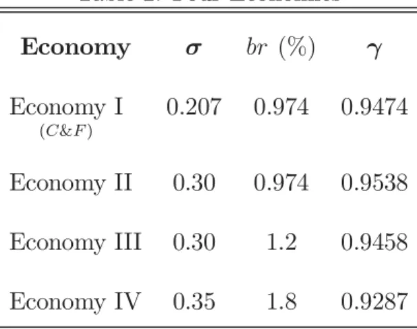
Table 2: Four Economies

Economy σ br (%) γ

Economy I

(C&F)

0.207 0.974 0.9474 Economy II 0.30 0.974 0.9538 Economy III 0.30 1.2 0.9458 Economy IV 0.35 1.8 0.9287

Hence Economy II departs from the Carlstrom and Fuerst economy by having greater uncertainty in the technology shock but holds the bankruptcy rate at the same level used by Carlstrom and Fuerst (note that this implies that the internal rate of return ³

1 γ

´ to en- trepreneurs falls). Economy III then permits the bankruptcy rate to increase by roughly a third. The final economy increases both the degree of technological uncertainty and the steady-state bankruptcy rate. To examine the effects of these changes, Table 3 reports the behavior of several key variables; for all but two variables, these are presented as percentage

11 The equations defining the steady-state are presented in the Appendix. This derivation also demon- strates that the parameterη(the fraction of entrepreneurs in the economy) is strictly a normalization and does not influence equilibrium characteristics.

12 In Table 2, the values of γ are reported strictly for comparison. That is, once the values ofσandbr are specified, the value ofγis determined endogenously.

deviations from the values in the Carlstrom and Fuerst economy. The risk premium differ- ential is reported as an absolute change while the minimum technology shock defined in the lending contract (i.e. ω) in the three modified economies is reported ¯

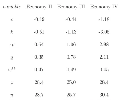
Table 3: Steady-state behavior

variable Economy II Economy III Economy IV

c -0.19 -0.44 -1.18

k -0.51 -1.13 -3.05

rp 0.54 1.06 2.98

q 0.35 0.78 2.11

¯

ω

0.47 0.49 0.45

z 28.4 25.0 28.4

n 28.7 25.7 30.4

Note that increases in uncertainty reduce the steady-state level of consumption and

the aggregate capital stock monotonically. For the high variance, high bankruptcy rate

economy (Economy IV), the reduction in consumption is greater than 1% - a non-trivial

amount and similar in magnitude to welfare losses reported by Lucas for moderate inflations

(Lucas (2000)). Clearly, more research is needed to examine the welfare consequences of

uncertainty - in particular, one of the lessons of the equity premium puzzle literature is

that logarithmic preferences are not consistent with agents’ treatment of aggregate risk;

introducing habit persistence or other preferences that more accurately represent agents’

risk tolerance would be a first step. We leave this to future research.

The risk premium associated with the lending contract as well as the price of capital are also monotonically increasing in the variance and the bankruptcy rate. However, note that this is not the case for the last three variables. In particular, the comparison between Economies II and III shows that holding the variance of the technology shock constant but increasing the steady-state bankruptcy rate results in a fall (again relative to Economy II) in both the entrepreneurs’ capital stock (z) and net worth (n). This occurs despite the fact that the price of capital is greater and reflects the impact that the greater bankruptcy rate has on the level of lending in the economy.

We now examine the cyclical behavior of the economy with time-varying uncertainty in the capital production sector.

3.2 Cyclical Behavior

As described in Section 2, eqs. (21)through (29) determine the equilibrium properties of the economy. To analyze the cyclical properties of the economy, we linearize (i.e. take a first-order Taylor series expansion) of these equations around the steady-state values. This

numerical approximation method is standard in quantitative macroeconomics. What is not

standard in this model is that the second moment of technology shocks hitting the capital

production sector will influence equilibrium behavior and, therefore, the equilibrium policy

rules. That is, linearizing the equilibrium conditions around the steady-state typically

imposes certainty equivalence so that variances do not matter. In this model, however, the

variance of the technology shock can be treated as an additional state variable through its role in determining lending activities and, in particular, the nature of the lending contract.

Linearizing the system of equilibrium conditions does not eliminate that role in this economy and, hence, we think that this is an attractive feature of the model.

While the previous section analyzed the steady-state behavior of four different economies, in this section we employ the same parameters as in the Carlstrom and Fuerst model (Econ- omy I in the previous section). We depart from Carlstrom and Fuerst by relaxing the i.i.d.

assumption for the capital sector technology shock. This is reflected in the law of motion for the standard deviation of the technology shock which is given in eq. (29); for convenience this is rewritten below:

σ

= ¯ σ

σ

µ

As in Carlstrom and Fuerst, the standard deviation of the technology shock ω

is, on average, equal to 0.207. That is, we set ¯ σ

= 0.207. We then examine two different economies characterized by the persistence in uncertainty, i.e. the parameter ζ. In the low persistence economy, we set ζ = 0.05 while in the high persistence economy we set ζ = 0.95.

The behavior of these two economies is analyzed by examining the impulse response functions of several key variables to a 1% innovation in σ

. These are presented in Figures 1-3.

We first turn to aggregate output and household consumption and investment. With

greater uncertainty, the bankruptcy rate increases in the economy (this is verified in Figure

2), which implies that agency costs increase. The rate of return on investment for the econ-

omy therefore falls. Households, in response, reduce investment and increase consumption

and leisure. The latter response causes output to fall. Note that the consumption and leisure response is increasing in the degree of persistence. This is not the case, however, for investment - this is due to the increase in the price of capital (see Figure 2) and reflects the behavior of entrepreneurs. This behavior is understood after first examining the lending channel.

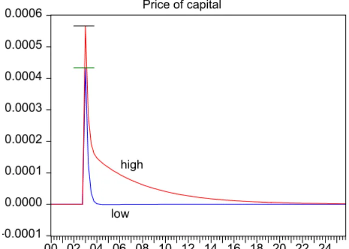
The increase in uncertainty affects, predictably, all three key variables in the lending channel: the price of capital, the risk premium associated with loans and the bankruptcy rate. As already mentioned, the bankruptcy rate increases and, in the high persistence economy, this increased rate of bankruptcy lasts for several quarters. This result implies that the bankruptcy rate is countercyclical in this economy; in contrast, in the analysis by Carlstrom and Fuerst the bankruptcy rate was, counterfactually, procyclical. Their focus was on the effects of innovation to the aggregate technology shock and, because of the assumed persistence in this shock, is driven by the change in the first moment of the aggregate production shock. Our analysis demonstrates that second moment effects may play a significant role in these correlations over the business cycle. Further research, both empirical and theoretical, in this area would be fruitful . Returning to the model, the increased bankruptcy rate implies that price of capital is greater and this increase lasts longer in the high persistence economy. The same is true for the risk premium on loans.

Figure 3 reports the consumption and net worth of entrepreneurs in the economies. In contrast to all other variables, persistence has a dramatic qualitative effect on entrepreneurs’

behavior. With low persistence, entrepreneur’s exploit the high price of capital to increase

consumption: the lack persistence provides no incentive to increase investment. Since the

price of capital quickly returns to its steady-state values, the increased consumption erodes

entrepreneurs’ net worth. To restore net worth to its steady-state value, consumption falls

temporarily. The behavior in the high persistence economy is quite different: the price

of capital is high and forecast to stay high so investment increases dramatically. Initially,

the investment is financed by lower consumption, but as entrepreneurs net worth increases

(due to greater capital and a higher price of capital) consumption also increases. This

endogenous response by entrepreneurs is why, in the high persistence economy, the initial

fall in aggregate investment is not as great in the high persistence economy.

Figure 1: Impulse Response Functions Output, Consumption, Investment

-0.0008 -0.0006 -0.0004 -0.0002 0.0000

00 02 04 06 08 10 12 14 16 18 20 22 24 Output

low high

-0.0001 0.0000 0.0001 0.0002 0.0003 0.0004 0.0005

00 02 04 06 08 10 12 14 16 18 20 22 24 Consumption

low

high

-0.005 -0.004 -0.003 -0.002 -0.001 0.000 0.001

00 02 04 06 08 10 12 14 16 18 20 22 24 high

low

Investment

Figure 2: Impulse Response Functions Price of Capital, Risk Premium, Bankruptcy Rate

-0.0001 0.0000 0.0001 0.0002 0.0003 0.0004 0.0005 0.0006

00 02 04 06 08 10 12 14 16 18 20 22 24 Price of capital

low high

-0.0002 0.0000 0.0002 0.0004 0.0006 0.0008

00 02 04 06 08 10 12 14 16 18 20 22 24 Risk Premium

low high

Bankruptcy Rate

-0.00005 0.00000 0.00005 0.00010 0.00015 0.00020 0.00025 0.00030

00 02 04 06 08 10 12 14 16 18 20 22 24 high

low

Figure 3: Impulse Response Functions Entrepreneurs’ Consumption, Net Worth

-0.002

00 02 04 06 08 10 12 14 16 18 20 22 24 0.000

0.002 0.004

0.006 Net Worth

high

low

-0.06 -0.04 -0.02

00 02 04 06 08 10 12 14 16 18 20 22 24 high

Entrepreneurs' Consumption low

0.00 0.02 0.04

4 Conclusion

The effect of uncertainty as characterized by second moment effects has been largely ignored in quantitative macroeconomics due to the numerical approximation methods typically em- ployed during the computational exercise. The analysis presented here uses standard solu- tion methods (i.e. linearizing around the steady-state) but exploits features of the Carlstrom and Fuerst (1997) agency cost model of business cycles so that time varying uncertainty can be analyzed. While development of more general solution methods that capture second moments effects is encouraged, we think that the intuitive nature of this model and its stan- dard solution method make it an attractive environment to study the effects of time-varying uncertainty.

Our primary findings fall into three broad categories. First, we demonstrate that un-

certainty affe cts the le ve l o f the ste ady-sta t e of t he e c ono my s o that wel f are ana ly se s of

uncertainty that focus entirely on the variability of output (or consumption) will understate

the true costs of uncertainty. Second, we demonstrate that time varying uncertainty results

in countercyclical bankruptcy rates - a finding which is consistent with the data and opposite

the re sult in C arl strom and Fu erst. Thi rd , we s how tha t p e rsi sten ce of unce rtai nty affects

both quantitatively and qualitatively the behavior of the economy. Together, these results

make a strong case for more research into the effects that uncertainty have on economic

behavior.

References

Alderson, M.J. and B.L. Betker (1995) “Liquidation Costs and Capital Structure,”

Journal of Financial Economics, 39, 45-69.

Altman, E. (1984) “A Further Investigation of the Bankruptcy Cost Question,” Journal of Finance, 39, 1067-89.

Carlstrom, C. and T. Fuerst (1997) “Agency Costs, Net Worth, and Business Fluctua- tions: A Computable General Equilibrium Analysis,” American Economic Review, 87, 893-910.

Collard, F. and M. Juillard, “A Higher-Order Taylor Expansion Approach to Simu- lation of Stochastic Forward—Looking Models with an Application to a Non—Linear Phillips Curve,” Computational Economics, forthcoming.

Lucas, R.E., Jr.(1987), “Models of business cycles ,” Oxford, OX, UK ; Cambridge, Mass., USA : B. Blackwell Publishers.

Lucas, R.E., Jr. (2000), “Inflation and Welfare,” Econometrica, 68(2), 247-274.

Obstfeld, M. and K. Rogoff (2000) “New Directions for Stochastic Open Economy Models,” Journal of International Economics, 50, 117-153.

Schmitt-Grohe, S. and M. Uribe (2001), “Solving Dynamic General Equilibrium Models Using a Second-Order Approximation to the Policy Function,” University of Pennsyl- vania Department of Economics Working Paper.

Sims, C. (2001), “Second Order Accurate Solution of Discrete Time Dynamic Equilib- rium Models,” Princeton University Department of Economics Working Paper.

Williamson, S. (1987) “Financial Intermediation, Business Failures, and Real Business

Cycles,” Journal of Political Economy, 95, 1196-1216.

5 Appendix: Steady-state conditions in the Carlstrom and Fuerst Agency Cost Model

We first present the equilibrium conditions and express these in scaled (by the fraction of entrepreneurs in the economy) terms. Then the equations are analyzed for steady-state implications. As in the text, upper case variables denote aggregate wide while lower case represent household variables. Preferences and technology are:

U (˜ c, 1 − l) = ln ˜ c + ν (1 − l)

Y = θK

[(1 − η) l]

η

Where η denotes the fraction of entrepreneurs in the economy and θ is the technology shock. Note that aggregate household labor is L = (1 − η) l while entrepreneurs inelastically supply one unit of labor. We assume that the share of entrepreneur’s labor is approximately zero so that the production function is simply

Y = θK

[(1 − η) l]

This assumption implies that entrepreneurs receive no wage income (see eq. (9) in C&F.

There are nine equilibrium conditions:

The resource constraint

(1 − η) ˜ c

+ ηc

+ ηi

= Y

= θ

K

[(1 − η) l

]

(30)

Let c =

and h =

l, then eq(30) can be written as:

c

+ c

+ i

= θ

k

h

(31)

Household’s intratemporal efficiency condition

˜

c

= (1 − α)

ν K

[(1 − η) l

]

Defining ν

=

ν, this can be expressed as:

ν

c

= (1 − α) k

h

(32)

Law of motion of aggregate capital stock

K

= (1 − δ) K

+ ηi

[1 − Φ (¯ ω

) µ]

Dividing by η yields the scaled version:

k

= (1 − δ) k

+ i

[1 − Φ (¯ ω

) µ] (33)

Household’s intertemporal efficiency condition

q

1

˜ c

= βE

½ 1

˜ c

£ q

(1 − δ) + θ

αK

[(1 − η) l

]

¤ ¾

Dividing both sides by

and scaling the inputs by η yields:

q

1 c

= βE

½ 1 c

£ q

(1 − δ) + θ

αk

h

¤ ¾

(34)

The conditions from the financial contract are already in scaled form:

Contract efficiency condition

q

= 1

1 − Φ (¯ ω

) µ + φ (¯ ω

) µ

t)

(35)

Contract incentive compatibility constraint

i

n

= 1

1 − q

g (¯ ω

) (36)

Where n

is entrepreneur’s net worth.

Determination of net worth

ηn

= Z

£ q

(1 − δ) + θ

K

[(1 − η) l

]

¤

or, in scaled terms:

n

= z

£

q

(1 − δ) + θ

k

h

¤

(37)

Note that z

denotes (scaled) entrepreneur’s capital.

Law of motion of entrepreneur’s capital

Z

= ηn

½ f (¯ ω

) 1 − q

g (¯ ω

)

¾

− η c

q

Or, dividing by η

z

= n

½ f (¯ ω

) 1 − q

g (¯ ω

)

¾

− c

q

(38)

Entrepreneur’s intertemporal efficiency condition

q

= γβE

½ £

q

(1 − δ) + θ

αK

[(1 − η) l

]

¤ µ

q

f (¯ ω

) 1 − q

g (¯ ω

)

¶¾

Or, in scaled terms:

q

= γβ E

½ £

q

(1 − δ) + θ

αk

h

¤ µ

q

f (¯ ω

) 1 − q

g (¯ ω

)

¶¾

(39)

5.1 Definition of Steady-state

Steady-state is defined by time-invariant quantities:

c

= ˆ c, c

= ˆ c

, k

= ˆ k, ω ¯

= ˆ ω, h

= ˆ h, q

= ˆ q, z

= ˆ z, n

= ˆ n, i

= ˆ ı

So there are nine unknowns. While we have nine equilibrium conditions, the two in- tertemporal efficiency conditions become identical in steady-state since C&F impose the condition that the internal rate of return to entrepreneur is offset by their additional dis- count factor:

γ

µ qf ˆ (ˆ ω) 1 − qg ˆ (ˆ ω)

¶

= 1 (40)

This results in an indeterminacy - but there is a block recursiveness of the model due to the calibration exercise. In particular, we demonstrate that the risk premium and bankruptcy rate determine (ˆ ω, σ) - these in turn determine the steady-state price of capital.

From eq.(34) we have:

ˆ

q = αβ

1 − β (1 − δ) k ˆ

ˆ h

= αβ 1 − β (1 − δ)

ˆ y

k ˆ (41)

From eq.(32) we have:

ˆ h = 1 − α ν

k ˆ

ˆ h

ˆ

c = 1 − α ν

ˆ y ˆ

c (42)

From eq.(33) we have:

ˆ k = 1 − Φ (ˆ ω) µ

δ ˆ ı (43)

Note that these three equations are normally (i.e. in a typical RBC framework) used to find steady-state ³

ˆ k, ˆ h, ˆ c ´

- because q ˆ = 1. Here since the price of capital is endogenous, we have four unknowns.

From eq. (37) and eq. (34) we have ˆ

n = ˆ z µ

ˆ

q (1 − δ) + α y ˆ k ˆ

¶

= ˆ z q ˆ

β (44)

From eq. (38) and the restriction on the entrepreneur’s additional discount factor (eq.

(40)), we have

ˆ z = ˆ n 1

ˆ qγ − ˆ c

ˆ

q (45)

Combining eqs. (44) and (45) yields:

ˆ c

= 1

− β (46)

We have the two conditions from the financial contract ˆ

q = 1

1 − Φ (ˆ ω) µ + φ (ˆ ω) µ

(47) And

ˆ ı = 1

1 − q ˆ (1 − Φ (ˆ ω) µ − f (ˆ ω)) n ˆ (48) Finally, we have the resource constraint:

ˆ

c + ˆ c

+ ˆ ı = ˆ k

ˆ h

(49) The eight equations (41) , (42) , (43) , (44) , (45) , (47) , (48) , (49) are insufficient to find the nine unknowns. However, the risk premium, denoted as ζ, is defined by the following

ˆ q ω ˆ ˆ ı

ˆ ı − ˆ n = ζ (50)

But we also know (from eq.(48) that ˆ

n

ˆ ı = 1 − q ˆ (1 − Φ (ˆ ω) µ − f (ˆ ω)) = 1 − qg ˆ (ˆ ω) Rearranging eq.(50) yields:

ˆ q ω ˆ

ζ = 1 − n ˆ ˆ ı

substituting from the previous expression yields ˆ

ω = ζg (ˆ ω) (51)

Let κ = bankruptcy rate — this observable also provides another condition on the distri- bution. That is, we require:

Φ (ˆ ω) = κ (52)

The two equations eq.(51) and eq. (52) can be solved for the two unknowns - (ˆ ω, σ).

By varying the bankruptcy rate and the risk premium, we can determine different levels of uncertainty (σ) and the cutoff point (ˆ ω).

Note that the price of capital in steady-state, is a function of (ˆ ω, σ) as determined by eq. (47). The other preference parameter, γ is then determined by eq. (40). Once this is determined, the remaining unknowns: ³

ˆ

c, ˆ c

, ˆ h, ˆ ı, k, ˆ z, ˆ n ˆ ´

are determined by eqs.

(41) , (42) , (43) , (44) , (46) , (48) , (49).

Authors: Victor Dorofeenko, Gabriel S. Lee, Kevin D. Salyer

Title: Time-Varying Uncertainty and the Credit Channel

Reihe Ökonomie / Economics Series 118

Editor: Robert M. Kunst (Econometrics)

Associate Editors: Walter Fisher (Macroeconomics), Klaus Ritzberger (Microeconom ics)

ISSN: 1605-7996

© 2002 by the Department of Economics and Finance, Institute for Advanced Studies (IHS),

Stumpergasse 56, A-1060 Vienna • ( +43 1 59991-0 • Fax +43 1 59991-555 • http://www.ihs.ac.at