Universit¨ at Regensburg Mathematik
A coupled surface-Cahn-Hilliard bulk-diffusion system modeling lipid raft formation in cell membranes
Harald Garcke, Johannes Kampmann, Andreas R¨ atz and Matthias R¨ oger
Preprint Nr. 16/2015
MODELING LIPID RAFT FORMATION IN CELL MEMBRANES
HARALD GARCKE, JOHANNES KAMPMANN, ANDREAS R ¨ATZ, AND MATTHIAS R ¨OGER
Abstract. We propose and investigate a model for lipid raft formation and dynamics in biolog- ical membranes. The model describes the lipid composition of the membrane and an interaction with cholesterol. To account for cholesterol exchange between cytosol and cell membrane we cou- ple a bulk-diffusion to an evolution equation on the membrane. The latter describes a relaxation dynamics for an energy taking lipid-phase separation and lipid-cholesterol interaction energy into account. It takes the form of an (extended) Cahn–Hilliard equation. Different laws for the ex- change term represent equilibrium and non-equilibrium models. We present a thermodynamic justification, analyze the respective qualitative behavior and derive asymptotic reductions of the model. In particular we present a formal asymptotic expansion near the sharp interface limit, where the membrane is separated into two pure phases of saturated and unsaturated lipids, re- spectively. Finally we perform numerical simulations and investigate the long-time behavior of the model and its parameter dependence. Both the mathematical analysis and the numerical simulations show the emergence of raft-like structures in the non-equilibrium case whereas in the equilibrium case only macrodomains survive in the long-time evolution.
1. Introduction
Phase separation processes that lead to microdomains of a well-defined length-scale below the system size arise in various physical and biological systems. A prominent example is the microphase separation in block-copolymers [7] or other soft materials, characterized by a fluid- like disorder on molecular scales and high degree of order at larger scales. Here micro-scale pattern arise by a competition between thermodynamic forces that drive (macro-)phase separation and entropic forces that limit phase separation. Different mathematical models for microphase separation in di-block copolymers have been developed, in particular built on self-consistent mean field theory (see for example [35] and the references therein) or density functional theory developed in [29, 39, 6] that leads to the so-called Ohta–Kawasaki free energy. Diblock-copolymer type models have also been studied on spheres and more general curved surfaces [32, 51, 10, 31]
and show a variety of different stripe- or spot-like patterns. In contrast to materials science microphase separation on biological membranes is much less understood, in particular in living cells. In this contribution we present and analyze a model for so-called lipid rafts, that represent microdomains of specific lipid compositions.
The outer (plasma) membrane of a biological cell consists of a bilayer formed by several sorts of lipid molecules and contains various other molecules like proteins and cholesterol. Besides being the physical boundary of the cell the plasma membrane also plays an active part in the functioning of the cell. Many studies over the past decades have shown that the structure of the outer membrane is heterogeneous with several microdomains of different lipid and/or protein composition. Such domains have been clearly observed in artificial membranes such as giant unilamellar vesicles [48, 49]. Here a ‘less fluidic’ (liquid-ordered) phase of saturated lipids and cholesterol separates from a ‘more fluidic’ (liquid-disordered) phase of unsaturated lipids. The nucleation of dispersed microdomains is followed by a classical coarsening process that leads to
Date: September 1, 2015.
2010Mathematics Subject Classification. 35K51, 35K71, 35Q92, 92C37, 35R37.
Key words and phrases. partial differential equations on surfaces, phase separation, Cahn–Hilliard equation, Ohta–Kawasaki energy, reaction-diffusion systems, singular limit.
1
coexisting domains with a length scale of the order of the system size. The situation is much more complex and much less understood for living cells. Their plasma membrane represents a heterogeneous structure with a complex and dynamic lipidic organization. The formation, maintenance and dynamics of intermediate-sized domains (10 - 200 nm on cells of µm size [30]) called ‘lipid rafts’ are of prime interest. These are characterized as liquid-ordered phases that consist of saturated lipids and are enriched of cholesterol and various proteins [44, 8]. These rafts contribute to various biological processes including signal transduction, membrane trafficking, and protein sorting [18]. It is therefore an interesting question to study the underlying process, by which these rafts are generated and maintained, and to understand the mechanism that allows for a dynamic distribution of intermediate-sized domains.
Several phenomenological mesoscale models have been proposed, see for example the review [18]. One class of models argues that raft formation is a result of a thermodynamic equilibrium process. Here one contribution is a phase separation energy that would induce a reduction of interfacial size between the raft and non-raft phases. The observation of nano-scale structures is then explained by including different additional energy contributions. One proposal is that thermal fluctuations near the critical temperature for the phase separation are responsible for the intermediate-sized structures. Other explanations consider interactions between lipids and membrane proteins that could act as a kind of surfactant or could ‘pin’ the interfaces due to their immobility [54, 46, 53]. Finally, raft formation could also be stabilized by induced changes of the membrane geometry and elasticity effects. However, as argued in [18], all such models are not able to reproduce key characteristics of raft dynamics; non-equilibrium effects essentially contribute to raft formation. Of particular importance are active transport processes of raft components that allow to maintain a non-equilibrium composition of the membrane. The competition between phase separation and recycling of raft components is argued to be of major importance for the dynamics and structure of lipid rafts.
Foret [20] proposed a simple mechanism of raft formation in a two-component fluid membrane.
This model includes a constant exchange of lipids between the membrane and a lipid reservoir as well as a typical phase separation energy. While relaxation of the latter tends to create large domains, the constant insertion and extraction of lipids in the membrane ensures indeed the formation of rafts. The emerging microdomains are static (in contrast to the lipid rafts on actual cell membranes) and the size distribution of these rafts is rather uniform, whereas in vivo cell membranes show a dynamic distribution of rafts of different sizes (see the concluding remarks in [20] and the discussion of Forets model in [18]). Moreover, as already noticed in [18], whereas Forets model is motivated by including non-equilibrium effects his model can be equivalently characterized as relaxation dynamics for an effective energy given by the Ohta–Kawasaki energy of block-copolymers [39] that is well-known to generate phase-separation in intermediate-sized structures.
A similar model by G´omez, Sagu´es and Reigada [22] considers a ternary mixture of saturated and unsaturated lipids together with cholesterol and studies the interplay of lipid phase sepa- ration and a continuous recycling of cholesterol. An energy that is determined by the relative concentration φ of saturated lipids and the relative cholesterol concentration c is proposed that in particular includes a phase separation energy of Ginzburg–Landau type for the lipid phases and a preference for cholesterol–saturated lipid interactions over cholesterol–unsaturated lipid interactions. The dynamics include an exchange term for cholesterol that is given by an in-/out- flux proportional to the difference from a constant equilibrium concentration of cholesterol at the membrane.
Our aim here is to propose an extended model and to present both a mathematical analysis and numerical simulations. Similar as in [22] one ingredient of our model are energetic contributions from lipid phase separation and lipid-cholesterol interaction. In addition, we include the dynam- ics of cholesterol inside the cytosol (the liquid matter inside the cell) and prescribe a detailed coupling between the processes in the cell and on the cell membrane. In particular, the outflow
of cholesterol from the cytosol appears as a source-term in the membrane-cholesterol dynamic and will be characterized by a constitutive relation. We will investigate different choices of this relation and will illustrate the implications on the emergence of microdomains.
1.1. A lipid raft model including cholesterol exchange and cytosolic diffusion. To give a detailed description of our model let us fix an open bounded setB ⊂R3 with smooth boundary Γ = ∂B representing the cell volume and cell membrane, respectively. Let ϕ denote a rescaled relative concentration of saturated lipid molecules on the membrane, with ϕ = 1 and ϕ = −1 representing the pure saturated-lipid and pure unsaturated-lipid phases, respectively. Moreover let v denote the relative concentration of membrane-bound cholesterol, where v = 1 indicates maximal saturation, and letudenote the relative concentration of cytosolic cholesterol. We then prescribe a phase-separation and interaction energy of the form
(1.1) F(v, ϕ) =
ˆ
Γ
ε
2|∇Γϕ|2+ε−1W(ϕ) + 1
2δ(2v−1−ϕ)2
dH2
with W a double-well potential that we choose as W(ϕ) = 14(1−ϕ2)2, constants ε, δ >0, and
∇Γ denoting the surface gradient. The first two terms represent a classical Ginzburg-Landau phase separation energy, whereas the third term models a preferential binding of cholesterol to the lipid-saturated phase. We define the chemical potentials
µ:= δF
δϕ =−ε∆Γϕ+ε−1W0(ϕ)−δ−1(2v−1−ϕ), (1.2)
θ:= δF δv = 2
δ(2v−1−ϕ), (1.3)
where ∆Γ denotes the Laplace–Beltrami operator on Γ, and prescribe for the dynamics of the concentrations over a time interval of observation (0, T) the following system of equations
∂tu=D∆u inB×(0, T],
(1.4)
−D∇u·ν =q on Γ×(0, T],
(1.5)
∂tϕ= ∆Γµ on Γ×(0, T],
(1.6)
∂tv= ∆Γθ+q= 4
δ∆Γv− 2
δ∆Γϕ+q on Γ×(0, T], (1.7)
where ν denotes the outer unit-normal field of B on Γ. The system is complemented with initial conditions u0, ϕ0, v0 for u, ϕ and v, respectively. The first equation represents a simple diffusion equation for the cholesterol in the bulk, the second equation characterizes the outflow of cholesterol. The third equation is a Cahn–Hilliard dynamics for the lipid concentration on the membrane, whereas the equation for the cholesterol on the membrane combines a mass-preserving relaxation of the interaction energy and an exchange with the bulk reservoir of cholesterol given by the flux from the cytosol. This combination yields a diffusion equation with cross-diffusion contributions and a source term.
To close the system it remains to characterize the exchange term q. We follow here two possibilities: First we prescribe a constitutive relation by considering the membrane attachment as an elementary ‘reaction’ between free sites on the membrane and cholesterol, and the detachment as proportional to the membrane cholesterol concentration, expressed by the choice
q = c1u(1−v)−c2v.
(1.8)
A similar coupling of bulk–surface equations has been investigated in a reaction-diffusion model for signaling networks [41, 42]. As a second possibility we consider choices of q that allow for a global free energy inequality for the coupled membrane/cytosol system. These two different cases could be considered as a distinction between open and closed systems and one important aspect of this work is to evaluate the consequences of these choices for the formation of complex phases.
We remark that the system conserves both the total cholesterol and the lipid concentrations since for arbitrary choices of q we obtain the relations
d dt
ˆ
B
u dx+ ˆ
Γ
v dH2
= 0, (1.9)
d dt
ˆ
Γ
ϕ dH2= 0.
(1.10)
Let us contrast the above model with the Ohta–Kawasaki model for phase separation in diblock copolymers mentioned above. Let Ω⊂Rn denote a spatial domain,ϕthe relative concentration of one of the two polymers and let m := ffl
ϕbe the prescribed average of ϕ over Ω. The mean field potential zis then given by
−∆z = ϕ−m in Ω, ∇z·νΩ = 0 on∂Ω, ˆ
Ω
z = 0.
Then a free energy is prescribed of the form FOK(ϕ) =
ˆ
Ω
ε
2|∇ϕ|2+ε−1W(ϕ)
dx+σ 2
ˆ
Ω
|∇z|2dx, (1.11)
where σ >0 is a fixed constant. Note that the last term can also be written as σ2kϕ−ffl
ϕk2H−1. A relaxation dynamics of Cahn–Hilliard type is then typically considered given as
∂tϕ = ∆µ, µ = δFOK
δϕ = −ε∆ϕ+ε−1W0(ϕ) +σz.
(1.12)
The energies F and FOK both contain a Cahn–Hilliard type energy contribution that favors macro-phase separation but are different in the additional terms. However we will see below that stationary patterns for our lipid raft model with the choice (1.8) are for smallδ >0 closely related to stationary points ofFOK. If on the other hand one considers simple choices forq that lead to a global free energy inequality, we will observe a macro-scale separation of all saturated lipids in one connected domain. This indicates that in fact non-equilibrium processes are responsible for lipid raft formation.
Several asymptotic regimes are interesting in view of the different parameters included in our model. We will investigate the limit ε → 0 that corresponds to a strong segregation limit and leads to a model where no mixing of the lipid phases is allowed and the domain splits into regions where ϕ = 1 and ϕ = −1 respectively. This limit corresponds to the sharp interface limit in phase-field models and connects to the analysis of the Ohta–Kawasaki model in [38]. Since the cytosolic diffusion in biological cells is known to be much faster than lateral diffusion on the cell membrane another natural reduction of the model appears in the limit D→ ∞ that leads to a non-local model defined solely on the cell membrane. Finally, assuming the effect of the lipid interaction with cholesterol to be large motivates to consider the asymptotic regime δ↓0.
1.2. Outline of the paper and main results. In the next section we will derive the model (1.4)-(1.7) from thermodynamic considerations. In particular we will show that for arbitrary choices of the exchange term q the surface equations and the bulk (cytosolic) equations are thermodynamically consistent when viewed as separate systems. Depending on the specific choice ofqwe may or may not have a global (that is with respect to the full model) free energy inequality.
We will present examples for both cases.
In Section 3 we will first derive a reduced raft model in the large cytosolic diffusion limit by formally taking D → ∞. We then analyze the qualitative behavior of the (reduced) system in terms of a characterization of stationary points and an investigation of their relation to stationary points of the Ohta–Kawasaki model. A formal asymptotic expansion for the sharp interface reduction ε → 0 of our raft model is presented in Section 4. Here we also briefly discuss the resulting limit problem that takes the form of a free boundary problem of Mullins–Sekerka type on the membrane with an additional coupling to a diffusion process in the bulk and including
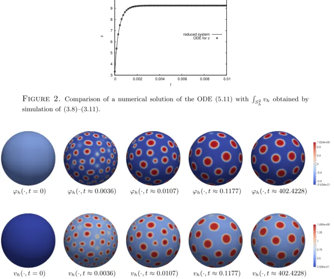
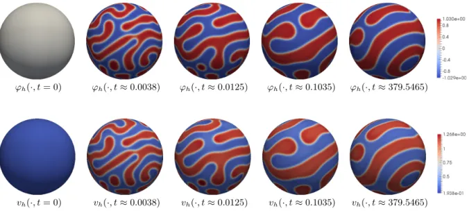
an interaction with the cholesterol concentration. In Section 5 we present numerical simulations of the full and reduced raft model. In particular, we study spinodal decomposition, coarsening scenarios and the possible appearance of raft-like structures as (almost) stationary states for different choices of the exchange term q and for different parameter regimes. Some conclusions are stated in the final section.
2. Thermodynamic justification of the lipid raft model
In this section we will derive the governing equations for the lipid raft model from basic thermodynamical conservation laws using a free energy inequality. Our arguments are similar to an approach used by Gurtin [24, 25], who derived the Cahn-Hilliard equation in the context of non-equilibrium thermodynamics. We first of all consider the equations which have to hold on the surface, will then consider the equations in the bulk and subsequently we will couple both systems.
The basic quantities on the membrane surface are the rescaled relative concentration of the saturated lipid molecules ϕ, the concentration v of the membrane-bound cholesterol, the mass fluxJϕ of the lipid molecules, the mass fluxJv of the cholesterol, the mass supply of cholesterolq, the surface free energy densityf and the chemical potential µrelated to the lipid molecules and the chemical potential θ related to the surface cholesterol. The underlying laws for any surface subdomain Σ⊂Γ are the mass balance for the lipids
(2.1) d
dt ˆ
Σ
ϕ dH2 =− ˆ
∂Σ
Jϕ·n dH1, the mass balance for the surface cholesterol
(2.2) d
dt ˆ
Σ
v dH2 =− ˆ
∂Σ
Jv·n dH1+ ˆ
Σ
q dH2
and the second law of thermodynamics, which in the isothermal situation has the form
(2.3) d
dt ˆ
Σ
f dH2 ≤ − ˆ
∂Σ
(µJϕ·n−(∂tϕf,∇Γϕ·n) +θJv·n)dH1+ ˆ
Σ
θq dH2
where f denotes the surface free energy density and where n is the outer unit conormal to ∂Σ in the tangent space of Γ. In addition, we denote by dHd the integration with respect to the d−dimensional surface measure and f,∇Γϕ denotes the partial derivatives off with respect to the variables related to ∇Γϕ in a constitutive relation f =f(...,∇Γϕ, ...). Similarly we will denote with a subscript comma partial derivatives with respect to other variables. For a discussion of these laws in cases in which source terms are present and at the same timef does not depend on
∇Γϕ we refer to [24], [26, Chapter 62], and [40]. Thermodynamical models of phase transitions with an order parameter typically involve a free energy density f which does depend on ∇Γϕ.
In this case the free energy flux does not only involve the classical terms µJϕ and θJv but also a term ∂tϕf,∇Γϕ. This is discussed in [25, 5, 2]. Gurtin [25] introduces a microforce balance involving a microstressξ in order to derive the Cahn-Hilliard equation. Here, we do not discuss the microforce balance and instead already use the form ξ = f,∇Γϕ which could be derived in our context in the same way as in [25]. However, in order to shorten the presentation we do not state the details. We hence obtain (2.3) as the relevant free energy inequality in cases where no external microforces are present.
Since the above (in-)equalities (2.1)–(2.3) hold for all Σ, we obtain with the help of the Gauß theorem on surfaces the local forms, compare [25],
∂tϕ+ divΓJϕ= 0 in Γ×(0, T], (2.4)
∂tv+ divΓJv=q in Γ×(0, T], (2.5)
∂tf + divΓ(µJϕ−∂tϕf,∇Γϕ+θJv)≤θq in Γ×(0, T].
(2.6)
With the constitutive relationf =f(v, ϕ,∇Γϕ) we obtain from the local form of the free energy inequality
f,ϕ∂tϕ+f,v∂tv+∇Γµ·Jϕ+∇Γθ·Jv+
(divΓJϕ)µ+ (divΓJv)θ−∂tϕdivΓf,∇Γϕ≤θq.
Using the conservation laws (2.4) and (2.5) we obtain
(f,ϕ−divΓ(f,∇Γϕ)−µ)∂tϕ+ (f,v−θ)∂tv+∇Γµ·Jϕ+∇Γθ·Jv ≤0.
The fact that solutions of the conservation laws with arbitrary values for∂tϕand∂tv can appear is used in the theory of rational thermodynamics to show that the factors multiplying∂tϕand∂tv have to disappear as they do not depend on∂tϕand ∂tv. We refer to Liu’s method of Lagrange multipliers [34] and to [26, 5] for a more precise discussion on how the free energy inequality can be used to restrict possible constitutive relations. We now choose the following constitutive relations which guarantee that the free energy inequality is fulfilled for arbitrary solutions of (2.4), (2.5). In fact, choosing
µ=f,ϕ−divΓ(f,∇Γϕ), (2.7)
θ=f,v, (2.8)
Jϕ=−Dϕ∇Γµ, (2.9)
Jv =−Dv∇Γθ (2.10)
withDϕ, Dv ≥0 ensures that the free energy inequality is fulfilled for all solutions of the conser- vation laws. More general models, e.g. taking cross diffusion into account, are possible and we refer to [5] for an approach which can be used to obtain more general models.
We now consider the governing physical laws in the bulk. As variables we choose u which is the relative concentration of the cytosolic cholesterol, the bulk chemical potential µu, the bulk free energy densityfb(u), the bulk fluxJu and the surface mass source termqu. We need to fulfill the following mass balance equation in integral form which has to hold for all openU ⊂B:
(2.11) d
dt ˆ
U
u dx=− ˆ
(∂U)\Γ
Ju·ν dH2+ ˆ
(∂U)∩Γ
qudH2 and the free energy inequality
(2.12) d
dt ˆ
U
fb(u)dx≤ − ˆ
(∂U)\Γ
µuJu·ν dH2+ ˆ
(∂U)∩Γ
µuqudH2
which also has to hold for all open U ⊂ B. Here we allowed for a source term qu on Γ and in accordance to our discussion above we introduced the free energy source µuqu in (2.12). As on the interface the free energy source term is given classically as a product of the mass source term and the chemical potential. If we use the fact that we can choose an arbitrary open setU which is compactly supported in B (which then implies (∂U)∩Γ = ∅) we obtain with the help of the Gauß theorem
∂tu+ divJu= 0 inB×(0, T], (2.13)
∂tfb(u) + div(µuJu)≤0 inB×(0, T].
(2.14) Choosing
µu =fb0(u), (2.15)
Ju =−M(u)∇(fb0(u)) (2.16)
makes sure that (2.14) is true for all solutions of (2.13). In the following we will often choose M(u) = fD00u
b(u) and this will lead to the linear diffusion equation (1.4)
∂tu−Du∆u= 0 inB×(0, T].
Choosing U such that∂U∩Γ6=∅ we obtain from (2.11) 0 =
ˆ
U
(∂tu+ divJu)dx= ˆ
∂U∩Γ
(qu+Ju·ν)dH2 which gives, since U is arbitrary,
qu =−Ju·ν (=Du∇u·ν) in Γ×(0, T],
and which yields (1.5) forq =−qu. We will now state global balance laws in the case where the mass supply for the interface stems from the bulk and vice versa.
Lemma 2.1. We assume that the above stated mass balance equations hold for the bulk and the surface and assume in addition thatqu=−q. Then it holds
d dt
ˆ
B
u dx+ ˆ
Γ
v dH2
= 0 d
dt ˆ
Γ
ϕ dH2 = 0.
If in addition, the free energy inequalities in the bulk and on the surface are true it also holds d
dt ˆ
Γ
f(v, ϕ,∇Γϕ)dH2+ ˆ
B
fb(u)dx
≤ ˆ
Γ
q(θ−µu)dH2.
Proof. The first two equations follow from (2.1), (2.2) with Σ = Γ and (2.11) with U =B since
∂U = Γ and since∂Γ =∅. The total free energy inequality follows similarly from (2.3) and (2.12).
Remark 2.2. (i) In the above lemma we chose qu = −q, that is the mass lost on the surface
generates a source of mass for the bulk.
(ii) Several constitutive laws for q make sense. It is possible to consider
(2.17) q=−c(θ−µu), c≥0
which leads to model for which the total free energy decreases. In this case we obtain d
dt ˆ
Γ
f(v, ϕ,∇Γϕ)dH2+ ˆ
B
fb(u)dx
≤ − ˆ
Γ
c(θ−µu)2dH2≤0.
(iii) We also consider the reaction type source term, compare (1.8), q =c1u(1−v) +c2v.
Also in this case we obtain a consistent model which fulfills the bulk and surface free energy inequalities with source terms as stated above. However, in this case the total free energy as the sum of the bulk and the surface free energy might increase which can be due to the fact that we neglect energy contributions generated by the detachment and attachment process.
(iv) One possible choice for the surface free energy density is, compare (1.1), f(v, ϕ,∇Γϕ) = γε
2 |∇Γϕ|2+ γ
εW(ϕ) + 1
2δ(2v−1−ϕ)2, ε, δ, γ >0.
Forfb(u) = 12u2,qu=−q and Du =D,γ =Dϕ=Dv = 1 we obtain the system (1.2)–(1.7).
With the above quadratic choice forfb and arguing as in the derivation of the energy inequality one can prove the identity
d dt
ˆ
Γ
ε
2|∇Γϕ|2+1
εW(ϕ) + 1
2δ(2v−1−ϕ)2dH2+ ˆ
B
1 2u2dx +
ˆ
Γ
(|∇Γµ|2+|∇Γθ|2)dH2+ ˆ
B
D|∇u|2 = ˆ
Γ
q(θ−u) (2.18)
where the last term is non-positive for the choice (2.17). Any other evolution that is based on a choice of q such that the right-hand side of (2.18) is always non-positive decreases the
total free energy. This is in particular the case for choices of q such that (1.2)-(1.7) can be characterized as a gradient flow.
In the following we are mainly interested in the dependence on the parameters ε, δ, Du and therefore as in (iv) above we always set Du = D, γ = Dϕ = Dv = 1, in which case the above choices of free energy densities and mass fluxes yield the system (1.2)–(1.7).
3. Qualitative behavior
In this section we will investigate qualitative properties of the model (1.2)-(1.7) and of the asymptotic reduction in the large cytosolic diffusion limit that we derive below. One key question here is whether or not our lipid raft model supports the formation of mesoscale patterns. We will distinguish different choices for the exchange termq and compare evolutions that reduce the total free energy with the evolution for the choice q given by the reaction-type law (1.8), which we consider as a prototype of a non-equilibrium model. We remark that most of the arguments in this section are purely formal; a rigorous justification is out of the scope of the present paper. In particular, we assume the existence of smooth solutions, their convergence to stationary states as times tends to infinity, and that the long-time behavior of the full system asymptotically agrees with that of the reduced system developed below.
We first observe that under an additional growth assumption on the exchange termqwe obtain energy bounds, even in the case that the system does not satisfy a global energy inequality.
Proposition 3.1. Assume thatq has at most linear growth, that is there exists Λ>0 such that
|q(ϕ, u, v)| ≤ Λ(1 +|ϕ|+|u|+|v|) for all ϕ, u, v∈R.
(3.1)
Then for all 0< t < T and all D≥D0 >0, 0 < ε≤ε0 any solution of (1.2)-(1.7) with initial dataϕ0, u0, v0 satisfies
F(v(·, t), ϕ(·, t)) + 1 2
ˆ
B
u(·, t)2+ ˆ t
0
ˆ
B
D
2|∇u|2 ≤ C(δ,Λ, T, D0, ε0, v0, ϕ0, u0).
(3.2)
Proof. From (2.18) we deduce that d
dt
F(v(·, t), ϕ(·, t)) + 1 2
ˆ
B
u(·, t)2 (3.3)
= − ˆ
B
D|∇u|2(·, t)− ˆ
Γ
|∇Γµ|2(·, t) +|∇Γθ|2(·, t)−(θ−u)(·, t)q(ϕ(·, t), u(·, t), v(·, t)) . For the last term we use the estimate
ˆ
Γ
(θ−u)q(ϕ, u, v) ≤
ˆ
Γ
θ2+u2+CΛ(1 +ϕ2+u2+v2)
= ˆ
Γ
θ2+CΛ
ˆ
Γ
(1 +ϕ2) + (CΛ+ 1) ˆ
Γ
u2+CΛ
ˆ
Γ
v2. (3.4)
For the second term on the right-hand side we obtain ˆ
Γ
(1 +ϕ2) ≤ C 1 + ˆ
Γ
W(ϕ)
≤ C(ε0) 1 +F(v(·, t), ϕ(·, t)) . (3.5)
Using [28, Chapter 2, (2.25)] the third term on the right-hand side of (3.4) can be estimated by bulk quantities,
ˆ
Γ
u2 ≤ D 2
ˆ
B
|∇u|2+C(D) ˆ
B
u2 for a suitable constant C(D), which in particular yields for all D≥D0
ˆ
Γ
u2 ≤ D 2
ˆ
B
|∇u|2+C(D0) ˆ
B
u2. (3.6)
To estimate the last integral on the right-hand side of (3.4) we first use Young’s inequality and (1.3) to obtain
16
δ2v2 = θ2+ 4
δθ(1 +ϕ) + 4
δ2(1 +ϕ)2 ≤ 2θ2+ 8
δ2(1 +ϕ)2, and further deduce that
v2 ≤ δ2
8 θ2+C(1 +W(ϕ)), ˆ
Γ
v2(·, t) ≤ C(δ, ε0)
1 +F(v(·, t), ϕ(·, t)) . (3.7)
We therefore obtain from (3.3)-(3.7) that d
dt
F(v(·, t), ϕ(·, t)) +1 2
ˆ
B
u(·, t)2 +D
2 ˆ
B
|∇u|2(·, t) + ˆ
Γ
|∇Γµ|2(·, t) +|∇Γθ|2(·, t)
≤C(δ,Λ, D0, ε0)
F(v(·, t), ϕ(·, t)) +1 2
ˆ
B
u(·, t)2
+C(δ,Λ).
By the Gronwall inequality we deduce the claim.
Note that for the choice (1.8) ofqassumption (3.1) is not satisfied. However, for any modification that coincides with that choice on a bounded domain in theu, vplane and that has at most linear growth outside the conclusion of Proposition 3.1 holds. For (2.17) or any other choice of q that implies a total free energy inequality we obtain an even better estimate, since now the right-hand side in (2.18) is non-positive.
3.1. A reduced model in the limit of large cytosolic diffusion. Since in the application to cell biology the bulk (cytosolic) diffusion is much higher than the lateral membrane diffusion a reasonable reduction of the model can be expected in the limit D→ ∞. In the case that the exchange term q satisfies assumption (3.1) we deduce by Proposition 3.1 that ´T
0
´
BD|∇u|2 is bounded uniformly in D. The same conclusion holds in the case of any free-energy decreasing evolution by (2.18). Therefore in the formal limitD→ ∞we conclude thatuis spatially constant and obtain the (non–local) system of surface PDEs
∂tϕ= ∆Γµ on Γ×(0, T],
(3.8)
µ=−ε∆Γϕ+ε−1W0(ϕ)−δ−1(2v−1−ϕ) on Γ×(0, T], (3.9)
∂tv= ∆Γθ+q= 4
δ∆Γv−2
δ∆Γϕ+q(ϕ, u, v) on Γ×(0, T].
(3.10)
This system is complemented by initial conditions for ϕ and v. The cholesterol concentration u=u(t) is determined by a mass conservation condition
(3.11)
ˆ
B
u(t) + ˆ
Γ
v(·, t) =M, whereM >0 is the total mass of cholesterol in the system.
Note that the transformation of the coupled bulk-surface system into a system only defined in the surface has the price of introducing a non-local term by the characterization ofuthrough the mass constraint. The reduction (3.8)-(3.11) is similar to the reduction to a shadow system for 2×2 reaction-diffusion systems introduced by Keener [27], see also the discussion in [37].
In the qualitative analysis below and the numerical simulations we will often restrict ourselves to the special choice q of the exchange function given in (1.8). For the reduced model it is then possible to compute the evolution of the total mass of u and v, which are related by (3.11). We
deduce, cf. (2.11), d
dt ˆ
B
u(t)dx = − ˆ
Γ
q(ϕ(·, t), u(t), v(·, t))dH2 = ˆ
Γ
−c1u(t)(1−v)(·, t) +c2v(·, t)dH2 (3.12)
= ˆ
Γ
(c1u(t) +c2)v(·, t)dH2−c1
|Γ|
|B|
ˆ
B
u(t)dx
= (c1u(t) +c2)
M− ˆ
B
u(t)dx
−c1|Γ|
|B|
ˆ
B
u(t)dx
= − c1
|B| ˆ
B
u(t)dx 2
+
c1
M− |Γ|
|B| −c2
ˆ
B
u(t)dx+c2M
and therefore we see that u(t) remains nonnegative if it was initially nonnegative (which is the relevant case) and converges fort→ ∞tou∞, which is the positive zero of
p(z) =−c1z2+ c1M− |Γ|
|B| −c2
z+c2M
|B| , thus
u∞ = 1 2
M − |Γ|
|B| −c2
c1 +
s 1 4
M− |Γ|
|B| −c2
c1 2
+ c2M c1|B|. (3.13)
Since p(0)>0 andp(|B|M )<0 we also obtain that ´
Γv(t) remains in [0, M] for all times.
We remark that ifq is given as in (1.8), then assumption (3.1) does not hold. Nevertheless we can obtain the reduced model for this particular choice of q if we start with a modified version:
Replace first q by
˜
q(u, v) = c1u−c1η(u)v−c2v,
where η : R → R is any smooth, monotone increasing and uniformly bounded function with η(r) =r for|r| ≤M|B|−1. Now the above arguments apply and we obtain the non-local model with exchange term ˜q. By analogous computations as above we then deduce
d dt
ˆ
B
u(t)dx= −c1|Γ|
|B| ˆ
B
u(t)dx+ c1η 1
|B|
ˆ
B
u(t)dx +c2
M− ˆ
B
u(t)dx , which yields 0 ≤ ´
Bu(t)dx ≤ M for all t ≥ 0 if this property holds for the initial data. But this implies ˜q(u(t), v(·, t)) =q(u(t), v(·, t)) for allt≥0. This justifies to consider in the following analysis and in the numerical simulations in Section 5 the exchange term q from (1.8) also for the non-local reduction.
3.2. Stationary points. We are in particular interested in the long-time behavior of solutions and will therefore next investigate stationary points of our lipid raft system. For the full system (1.2)-(1.7) stationary points (ϕ∞, u∞, v∞) are characterized by the equations
0 = ∆Γµ∞ on Γ,
0 = ∆Γθ∞+q(ϕ∞, u∞, v∞) on Γ, (3.14)
∆u∞= 0 inB, −D∇u∞·ν = q(ϕ∞, u∞, v∞) on Γ.
This implies thatµ∞ is constant and
−ε∆Γϕ∞+1
εW0(ϕ∞) = 1
δ(2v∞−1−ϕ∞) +µ∞ = θ∞
2 +µ∞, (3.15)
q(ϕ∞, u∞, v∞) = −2
δ∆(2v∞−1−ϕ∞), (3.16)
∆u∞= 0 in B, −D∇u∞·ν = q(ϕ∞, u∞, v∞) on Γ.
(3.17)
Alternatively, this system can be characterized by
−ε∆Γϕ∞+1
εW0(ϕ∞) = Q(ϕ∞) +µ∞, (3.18)
where Q(ϕ∞) = 12θ∞ is a nonlocal function of ϕ∞ as u∞, v∞ and hence θ∞ are determined by ϕ∞ through (3.16), (3.17).
3.3. The case of an energy-decreasing evolution. Let us in the following first consider the case that q is chosen such that the right-hand side in (2.18) is nonpositive, hence the total free energy is decreasing. For any stationary point u∞, v∞, ϕ∞ the energy inequality (2.18) yields that µ∞, θ∞ andu∞ are constant, in particular by (3.15)
−ε∆Γϕ∞+ 1
εW0(ϕ∞) = θ∞
2 +µ∞∈R, q(ϕ∞, u∞, v∞) = 0.
In addition, we fix the total lipid and cholesterol masses as they are for any evolution determined by the initial conditions. We therefore prescribe, forM, M1 given,
M = ˆ
B
u∞+ ˆ
Γ
v∞ = |B|u∞+ ˆ
Γ
v∞, M1 =
ˆ
Γ
ϕ∞.
In particular, the stationary stateϕ∞coincides with a critical point of the Cahn–Hilliard energy subject to a volume constraint. The conditionq = 0 provides an additional relation betweenϕ∞, u∞ and v∞. In the case of the exchange law (2.17) this determines´
Γv∞ and θ∞.
We can elaborate the connection with stationary points of the Cahn–Hilliard equation a bit more if we in addition assume that (u∞, v∞, ϕ∞) is a local minimizer of the energy (1.1). We represent the latter as
(3.19) F(v, ϕ) =F1(ϕ) +F2(v, ϕ),
where
F1(ϕ) :=
ˆ
Γ
ε
2|∇ϕ|2+ε−1W(ϕ), F2(v, ϕ) :=
ˆ
Γ
1
2δ(2v−1−ϕ)2. We also assume that both´
Γϕ∞and ´
Γv∞are fixed by the initial data and the conditionq = 0, which holds in particular in case of the exchange law (2.17).
For anyv, ϕwith ´
Γv=´
Γv∞ and ´
Γϕ=´
Γϕ∞ we then have ˆ
Γ
(2v−1−ϕ)2 = ˆ
Γ
2v−1−ϕ− − ˆ
(2v−1−ϕ) 2
+ ˆ
Γ
− ˆ
Γ
(2v−1−ϕ) 2
≥ ˆ
Γ
− ˆ
Γ
(2v∞−1−ϕ∞) 2
and deduce that under the respective mass constraints the minimizer of F2(v, ϕ) are given by those (v, ϕ) for which 2v−1−ϕis constant, and that the minimum only depends on ´
Γv and
´
Γϕ. Sinceθ∞ and thus 2v∞−1−ϕ∞ are constant, we see that u∞, v∞, ϕ∞minimizes F2. Moreover, for any ϕsatisfying the mass constraint the minimum ofF2 is attained byv= 12(1 + ϕ+ffl
(2v−1−ϕ)) and is independent ofϕ. Thereforeϕ∞as above needs to be a local minimizer of the Cahn–Hilliard energy F1 subject to a given mass constraint. In the case of the Cahn–
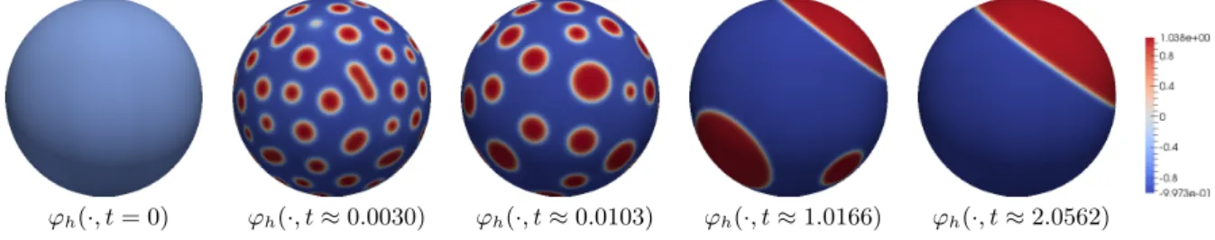
Hilliard dynamics in an open convex set in Rn, is is known [45] that stable stationary points converge in the sharp interface limitε→0 to configurations with one connected phase boundary of constant curvature. In analogy, one therefore might expect that for ε > 0 sufficiently small the only local minimizer in our lipid raft model for choices q that lead to an energy-decreasing evolution are given by configurations with one lipid phase concentrated in a single geodesic ball
on Γ. In particular, such local minimizer do not represent mesoscale pattern like lipid rafts. In Section 5.3.4 we present a numerical simulation for energy decreasing dynamics that confirms the expected behavior.
3.4. The case of the exchange term (1.8). Let us next discuss the choice of q as given in (1.8). The representation (3.18) shows some similarity to the equation for stationary points of the Ohta–Kawasaki model described above. We can make this more transparent in the case of the reduced system (3.8)-(3.11), at least if we presume that the long term behavior of the reduced systems captures the respective behavior of the full system (which means that the order of limits D→ ∞andt→ ∞can be interchanged). Sinceu∞is constant we obtain, writing ˜c1 =c1u∞for convenience, that
0 = ˆ
Γ
q(u∞, v∞) = |Γ|˜c1−(˜c1+c2) ˆ
Γ
v∞
(3.20) and further
q(u∞, v∞) = −c˜1+c2
2 (v∞−1−ϕ∞)− ˜c1+c2
2 (1 +ϕ∞) + ˜c1
= −δ(˜c1+c2)
4 θ∞−˜c1+c2
2 (1 +ϕ∞) + ˜c1
= −δ(˜c1+c2) 4
θ∞− θ∞
−δ(˜c1+c2) 4
2
δ (v∞−1−ϕ∞)−˜c1+c2
2 (1 +ϕ∞) + ˜c1
= −δ(˜c1+c2) 4
θ∞− θ∞
−˜c1+c2 2
ϕ∞− ϕ∞
, where we have used (3.20) in the third line. This implies by (3.14)
−∆Γ+δ(˜c1+c2) 4
θ∞− θ∞
= −˜c1+c2
2
ϕ∞− ϕ∞
. Since µ∞ is constant we deduce from equation (3.18)
−ε∆Γϕ∞+ε−1W0(ϕ∞) = µ∞+1
2 θ∞+ 1 2
θ∞− θ∞
= µ∞+1
2 θ∞− ˜c1+c2
4
−∆Γ+ δ(˜c1+c2) 4
−1
ϕ∞− ϕ∞
. Forδ 1 this can be approximated by
−ε∆Γϕ∞+ε−1W0(ϕ∞) +˜c1+c2
4 (−∆Γ)−1
ϕ∞− ϕ∞
= µ∞+1 2 θ∞. (3.21)
The latter equation corresponds to stationary points of the Ohta–Kawasaki functional FOK(ϕ) =
ˆ
Γ
ε
2|∇ϕ|2+ε−1W(ϕ)
+σ
2kϕ− ϕk2H−1
(3.22) with
(3.23) σ = ˜c1+c2
4 ,
where the constant on the right-hand side of (3.21) should be interpreted as a Lagrange multiplier associated to a mass constraint for ϕ.
The total lipid mass´
ϕis given by the initial data. We can also identify ˜c1+c2 as a function of the data. First its value is characterized byu∞ and using (3.13) we deduce
˜
c1+c2 = 1 2
c2+ M
|B|c1− |Γ|
|B|c1
+
s 1 4
c2+ M
|B|c1− |Γ|
|B|c1
2
+c1c2
|Γ|
|B|. (3.24)
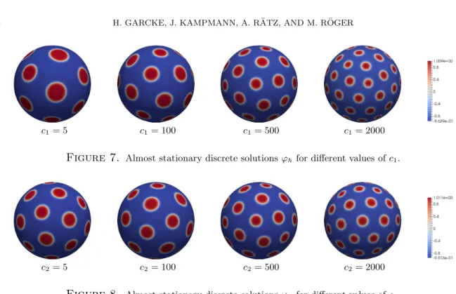
In Section 5.3.2 we will present simulations that confirm that the long-time behavior of the reduced system is for δ 1 in fact very close to that of the Ohta–Kawasaki dynamics. In particular, in contrast to any choice of q that induces an energy-decreasing evolution, in the case of the exchange term (1.8) we in fact see the occurrence of mesoscale patterns.
Remark 3.2. Let us highlight one key difference in the long-time behavior of our model in the different cases considered above. For a free-energy decreasing evolution stationary states are characterized by the properties thatθ∞ is constant andq∞=q(ϕ∞, u∞, v∞) zero. For the choice (1.8) of the exchange term on the other hand and the reduced system we have stationary states with non-vanishing q∞, which correspond to an persisting exchange of cholesterol between bulk and cell membrane. This process eventually allows for the formation of complex pattern on a mesoscopic scale.
4. Sharp interface limit ε→0 by formally matched asymptotic expansions In this section we formally derive the sharp interface limit of the diffuse interface model (1.2)–
(1.7) asε→0.We assume throughout this section that the tuple (uε, ϕε, vε, µε, θε) solves (1.2)–
(1.7) and converges formally asε→0 to a limit (u, ϕ, v, µ, θ). Furthermore, we suppose that the family of the zero level sets of the functions ϕε converges as ε → 0 to a sharp interface. This interface, at times t∈[0, T] is supposed to be given as a smooth curve γ(t)⊂Γ which separates the regions {ϕ(·, t) = 1} and {ϕ(·, t) =−1}. By a formal asymptotic analysis, we conclude that the limit functions (u, ϕ, v, µ, θ) can be characterized as the solutions of a free boundary problem on the surface Γ, which is again coupled to a diffusion equation in the bulkB. Other examples for this method and more details on formal asymptotic analysis can be found in [2, 4, 9, 19, 21]
which is by far not a comprehensive list of references.
The obtained limit problem describes a time-dependent partition of the surface Γ into different phase regions
Γ+(t) := {ϕ(·, t) = 1} and Γ−(t) := {ϕ(·, t) =−1}
(4.1)
and the dynamic of the interface γ(t) between these two regions. We denote the corresponding separation of the surface-time domain Γ×(0, T] by
Γ± := {(x, t)∈Γ×(0, T] : x∈Γ±(t)}.
The limit problem then takes the following form.
Sharp Interface Problem 4.1. The sharp interface model obtained from the formal asymptotic analysis is given by
ϕ=±1 on Γ±,
(4.2)
∂tu=D∆u in B×(0, T],
(4.3)
−D∇u·ν =q:=c1u(1−v)−c2v on Γ×(0, T], (4.4)
∆Γµ= 0 on Γ±,
(4.5)
∂tv= ∆Γθ+q on Γ±,
(4.6)
θ= 2
δ(2v−1∓1) on Γ±,
(4.7)
2µ+θ=c0κg on γ,
(4.8)
[µ]+− = 0 on γ,
(4.9)
[θ]+− = 0 on γ,
(4.10)
−2V = [∇Γµ]+−·νγ on γ, (4.11)
−V = [∇Γθ]+−·νγ on γ, (4.12)
where [·]+− is the jump across the interface γ and νγ(x0, t0) ∈ Tx0Γ denotes the unit normal to γ(t0) in x0 ∈ γ(t0), pointing inside Γ+(t0). The geodesic curvature of γ(t) in Γ is denoted by κg(·, t) and V(x0, t0) denotes the normal velocity of γ(t0) inx0 ∈γ(t0) in direction of νγ(x0, t0).
For its precise definition, letγt:U →γ(t)⊂Γ,t∈(t0−δ, t0+δ) be a smoothly evolving family of local parameterizations of the curves γ(t) by arc length over an open interval U ⊂ Rand let γt0(s0) =x0. Then the normal velocity in (x0, t0) is given by
V(x0, t0) = d dt t0
γt(s0)·νγ(x0, t0), see also [11].
We first deduce the existence of transition layers between the phase regions. By assuming that the functions (uε, ϕε, vε, µε, θε) admit suitable expansions with respect to the parameterεin the transitions layers and in the regions away from the interface respectively, we can then deduce that the limit functions at least formally need to fulfill (4.2)–(4.12).
4.1. Asymptotic analysis: Existence of transition layers and outer expansion. We start our analysis by expanding the solutions to the coupled model in the outer regions, whereϕε attains values away from zero. We assume that in these regions all functions in (1.2)–(1.7) have expansions of the form
fε=
∞
X
k=0
εkfk wherefε =ϕε, vε, . . . ,etc.
Since we postulated the existence of different phase regions characterized by the values of the limit function ϕ, we should first address the existence of these phase regions. To this end, we collect all terms of order ε−1 in (1.2) and obtain
W0(ϕ0) = 0
and as a consequence we obtainϕ0 =±1 as the only stable solutions. Sinceϕ0 is the dominant term in the assumed expansion as ε→ 0, we deduceϕε→ ±1 as ε→ 0 and the existence of the claimed transition layers. This justifies (4.1) and (4.2).
The discussion of equations (1.3) and (1.4)–(1.7) is then straightforward. Comparing the terms of order O(1) in their corresponding equations allows us to deduce (4.3)–(4.7).
Due to the (possibly steep) transition between the regions Γ+ and Γ− near the interface, the spatial derivatives occurring in the system might contribute terms which are not necessarily of order O(1) (with respect to ε) in a neighborhood of the interface. This motivates the need for a more detailed analysis of the functions in the neighborhood of the interface which we will address in Section 4.3.
4.2. Coordinates for a neighborhood of the interface. As stated above, we suppose that the zero level sets ofϕεconverge to some (smooth) curveγ(t) with inner (wrt. Γ+(t)) unit normal field νγ(·, t). We then introduce on a small tubular neighborhood N of γ(t) a new coordinate system which is more suitable for the analysis in the transition layer. We remark that the construction of these coordinates presented here is more complicated which is due to the fact that N is a neighborhood ofγ(t) in the manifold Γ.For a similar example, we refer the reader to [17].
As above, letγt:U →γ(t) be a local parametrization of the curve γ(t) by arc length over an open intervalU ⊂R.It is then possible to extendγtto a local parametrization ΨtofN by means of the exponential map from differential geometry.
While details on this map can be found in the literature [12, 13], it is sufficient for our purpose to quickly recall its definition. For a given point p ∈ Γ and a vector ~a ∈ TpΓ, there exists a unique geodesic curve c~a such that c~a(0) =p and c~0a(0) =~a. The exponential map expp in p is then defined for all~a∈TpΓ for whichc~a(1) exists and is given by expp(~a) =c~a(1). Note that for z∈[0,1] one can easily check expp(z~a) =c~a(z).
The distance between a point x∈Γ and the interfaceγ(t) is defined as d(x, t) := inf{l(c)|c:I →Γ, c connectsx and γ(t)} wherel(c) denotes the length of the curve c.Setting
Ψt(s, r) = expγt(s)(rνγ(γt(s), t)),
we obtain that Ψt is a parametrization of a neighborhood N(t) of γ(t). If we chooseN(t) small enough, the properties of the exponential map imply that r is the signed distance between the point Ψt(s, r) and γ(t),that is for (x, t) = Ψt(s, r)∈N(t) we have
r=d(x, t) :=b
(d(Ψt(s, r), t) ifr ∈Γ+(t)
−d(Ψt(s, r), t) ifr∈Γ−(t).
For the asymptotic analysis, it is necessary to adapt the parametrization to the length scale of the transition layers. We therefore use the rescaled parametrization
(4.13) Λ(s, z, t) = Ψt(s, εz)
of N(t),where z= rε.In particular, z can be written as a function ofx andt.
Let us remark that as γ(t) is the zero level set of the signed distance functiond,b the tangent space ofγ(t) is the subspace of the tangent space of Γ which is orthogonal to the surface gradient
∇Γdband thus the normal vector νγ ofγ(t) is given by ∇Γdb
k∇ΓdbkΓ.Because of 0 = d
dtd(γb t(s), t) =∇Γd(γb t(s), t)·∂tγt(s) +∂td(γb t(s), t) we can thus compute
∂tγt(s)·ν =− ∂td(γb t(s), t)
∇Γd(γb t(s), t) Γ
and therefore the time derivative∂tz on γ(t) fulfills
∂tz=−ε−1V.
Remark 4.2 (Gradient, Divergence and Laplace Operator in the new coordinates). From the definition of Λ in (4.13) we see
Λ(s,0, t) =γt(s), (4.14)
∂sΛ(s,0, t) =∂sγt(s) =γt0(s) and (4.15)
∂zΛ(s,0, t) =ενγ(γt(s)).
(4.16)
Furthermore, the curver 7→Ψt(s, r) is geodesic by definition and hence we have P∂zzΛ(s, z, t) = 0
whereP is the projection on the tangent spaceTΛ(s,z,t)Γ on Γ in Λ(s, z, t).
These observations allow us to calculate
∂z(∂sΛ(s, z, t)·∂zΛ(s, z, t)) =∂zsΛ(s, z, t)·∂zΛ(s, z, t) +∂sΛ(s, z, t)·∂zzΛ(s, z, t)
= 1
2∂s|∂zΛ(s, z, t)|2 = 0
since |∂zΛ(s, z, t)|2 = ε2 by definition. The equations (4.15) and (4.16) imply ∂sΛ(s,0, t) ·
∂zΛ(s,0, t) = 0,which yields
(4.17) ∂sΛ(s, z, t)·∂zΛ(s, z, t) = 0.
For simplification of the following calculations, we denote the variables s and z by s1 and s2
respectively. Given the arguments above, the metric tensor with respect to Λ is given by g11=gss=∂sΛ·∂sΛ,
g12=g21=gsz =gzs=∂sΛ·∂zΛ = 0 and g22=gzz =∂zΛ·∂zΛ =ε2.
The matrix
G:=
g11 g12 g21 g22
is thus diagonal and as usual we denote the entries of its inverse G−1 by gij.
For a scalar functionh(x, t) =bh(s(t, x), z(t, x), t) onN, the surface gradient onN ⊂Γ is hence expressed by
∇Γh=
2
X
i,j=1
gij∂sibh∂sjΛ =g11∂s1bh∂s1Λ + 1
ε2∂s2bh∂s2Λ =∇γεbh+1
ε∂zbh∂zΛ (4.18)
where∇γε is the surface gradient onγε={Λ(s, z, t)|s∈U} for a fixedz∈[0,1].Similarly,
∇Γ·a=∇γε·ba+ 1
ε∂zba·∂zΛ (4.19)
for some vector valued function a(x, t) =ba(s(x, t), z(x, t), t).
In analogy to the appendix in [2], we calculate the Laplace-Beltrami operator ∆Γ in the new coordinates. Due to the properties of the parametrization Λ(s, z, t) which already lead to the diagonal structure of the metric tensor above, we find∇γεbh·∂zΛ = 0 and∇γεbh·∂zzΛ = 0.Hence
∂z∇γεbh
·∂zΛ =
∂z∇γεbh
·∂zΛ +∇γεbh·∂zzΛ =∂z
∇γεbh·∂zΛ
= 0 and substituting (4.18) in (4.19) we thus compute
∆Γh=∆γεbh+1 ε
∇γε∂zbh
·∂zΛ +1
ε∂zbh∇γε·∂zΛ +1
ε
∇∂zγεbh
·∂zΛ + 1
ε2∂zzbh·∂zΛ + 1
ε2∂zbh∂zzΛ·∂zΛ
=∆γεbh+1
ε∂zbh∇γε·∂zΛ + 1
ε2∂zzbh·∂zΛ (4.20)
where we have used the identities above. Since
∂ssΛ·∂sΛ = 1
2∂s(∂sΛ·∂sΛ) = 0,
the curvature vector∂ssΛ ofγ(t) (seen as a curve in R3) is an element in span (∂zΛ, νΓ) whereνΓ denotes the direction normal to the surface Γ.The geodesic curvatureκg ofγ(t) in Γ is therefore given by
κg =∂ssΛ·∂zΛ =∂s(∂sΛ·∂zΛ)−∂sΛ·∂szΛ =−∇γε·∂zΛ.
As in [2], one can derive
∇γεbh=∇γbh+Rε
∇γε·bh=∇γ·bh+Rε
∆γεbh= ∆γbh+Rε