Universit¨ at Regensburg Mathematik
A stable numerical method for
the dynamics of fluidic membranes
John W. Barrett, Harald Garcke and Robert N¨ urnberg
Preprint Nr. 18/2014
A Stable Numerical Method for the Dynamics of Fluidic Membranes
John W. Barrett
†Harald Garcke
‡Robert N¨ urnberg
†Abstract
We develop a finite element scheme to approximate the dynamics of two and three dimensional fluidic membranes in Navier–Stokes flow. Local inextensibility of the membrane is ensured by solving a tangential Navier–Stokes equation, taking surface viscosity effects of Boussinesq–Scriven type into account. In our approach the bulk and surface degrees of freedom are discretized independently, which leads to an unfitted finite element approximation of the underlying free boundary problem.
Bending elastic forces resulting from an elastic membrane energy are discretized us- ing an approximation introduced by Dziuk (2008). The obtained numerical scheme can be shown to be stable and to have good mesh properties. Finally, the evolution of membrane shapes is studied numerically in different flow situations in two and three space dimensions. The numerical results demonstrate the robustness of the method, and it is observed that the conservation properties are fulfilled to a high precision.
Key words. fluidic membranes, incompressible two-phase flow, parametric finite elements, virtual element method, Helfrich energy, Boussinesq–Scriven surface fluid, local surface area conservation
AMS subject classifications. 65M60, 65M12, 76M10, 76Z99, 92C05, 35Q35, 76D05
1 Introduction
The evolution of lipid bilayer membranes is driven by the bending energy, which involves the curvature of the membrane, and hydrodynamics. Lipid membranes typically form vesicles, i.e. bag-like structures containing fluid, which are surrounded by a possibly dif- ferent fluid. The omnipresence of membranes in biological systems has led to a growing
†Department of Mathematics, Imperial College London, London, SW7 2AZ, UK
‡Fakult¨at f¨ur Mathematik, Universit¨at Regensburg, 93040 Regensburg, Germany
interest in vesicles over the past decades. Much of the work on vesicles was motivated by the fact that their shape at rest resembles the biconcave forms of red blood cells. It is the goal of this paper to introduce, and analyze, a finite element method of a model for the evolution of lipid membranes, which was introduced by Arroyo and DeSimone (2009).
The bending energy for a lipid membrane used in this paper is Eα(Γ) =α E(Γ), with E(Γ) = 12
Z
Γ
κ2 dHd−1,
where the bilayer is modelled as a closed hypersurface Γ inRd,d= 2 or 3. Byκ we denote the mean curvature (the sum of the principal curvatures) of Γ, α ∈ R>0 is the bending rigidity and dHd−1 indicates integration with respect to the (d−1)-dimensional surface measure. In the simplest energetical model for vesicles one minimizes the energy Eα(Γ) under the constraints that the area of Γ is fixed and that Γ encloses a fixed volume.
The latter is due to the fact that the osmotic conditions of the fluids surrounding the membrane lead to a fixed volume. Furthermore, the vesicle can be considered as locally incompressible, which leads to a fixed total surface area. For a deeper physical discussion of these conditions we refer to the overview article of Seifert (1997), where also other aspects of fluidic membranes and vesicles are thoroughly discussed.
In the fluid regions, Ω− and Ω+, inside and outside of the membrane, one requires the incompressible Navier–Stokes equations, i.e.
ρ(~ut+ (~u .∇)~u)− ∇. σ =ρ ~f , ∇. ~u= 0.
At typical temperatures the membrane itself is in a fluidic state, which leads to the fact that on the membrane the incompressible surface Navier–Stokes equations
ρΓ∂t•~u− ∇s. σΓ = [σ ~ν]+−+α fΓ~ν, ∇s. ~u= 0
have to hold. Here σΓ is the surface stress tensor, ~ν is the unit normal on Γ and [σ ~ν]+− describes stresses acting on the membrane via the normal stresses σ ~ν from both sides of the membrane (see Section 2 for precise definitions). The operator ∇s. is the surface divergence and ∇s. ~u= 0 models the fact that the membrane is locally incompressible.
Interfacial fluid mechanics was first thoroughly discussed by Scriven (1960), general- izing earlier ideas of Boussinesq. In this context the surface stress tensor σΓ was first introduced, and is hence called the Boussinesq–Scriven tensor. In addition,α fΓ~ν models forces acting on the membrane, which result from the curvature elasticity Eα(Γ). The forces act in a direction normal to the membrane and fΓ is given as minus the first variation of E(Γ), i.e.
fΓ =−∆sκ−κ|∇s~ν|2+ 12κ3, (1.1) where ∆s is the surface Laplacian and∇s is the surface gradient.
In recent years, many papers have appeared which numerically approximate the L2- gradient flow equation related to the Willmore energy E(Γ), i.e.
V =−∆sκ−κ|∇s~ν|2+12κ3, (1.2)
where V is the normal velocity of the evolving membrane Γ. This geometric evolution equation is called Willmore flow, and we refer to Mayer and Simonett (2002); Clarenzet al.
(2004); Dziuk (2008); Barrettet al.(2008b); Deckelnick and Dziuk (2009); Deckelnick and Schieweck (2010); Barrettet al. (2012); Franken et al.(2013) for different computational approaches to Willmore flow. Since the enclosed volume and the total surface area are preserved for lipid membranes, the volume and area preserving variant of (1.2), which is called Helfrich flow, is of particular interest. Helfrich flow has been considered numeri- cally in e.g. Barrettet al.(2008b); Bonitoet al.(2010). Other authors included additional physical effects in the geometrical model, such as lateral inhomogeneity and line tension effects, see Elliott and Stinner (2010); Mercker et al. (2013). Bonito et al. (2011) con- sidered a fluid-membrane system in which forces resulting from the Willmore energy act on an interior flow. In their model surface area is maintained with the help of a global Lagrange multiplier.
As pointed out above, the membrane is locally incompressible and hence the condi- tion ∇s. ~u = 0 should be enforced on the flow. This condition has been dealt with in numerical simulations by Salac and Miksis (2011, 2012); Laadhari et al. (2014) within a level set context, by Jamet and Misbah (2007); Aland et al. (2014) with the help of a phase field approach and by Hu et al. (2014) using an immersed boundary method. In these approaches the local incompressibility constraint on the membrane is enforced by a Lagrange multiplier leading to an inhomogeneous surface pressure. However, in the computations in the latter paper the constraint is relaxed by a spring-like elastic force.
In addition, there exists work on the surface Stokes system without taking the bulk fluid flow into account. There the volume conservation is enforced by a global Lagrange multi- plier. We refer to Rahimi and Arroyo (2012); Rodrigueset al.(2014) for numerical results using this modelling variant. The only numerical work taking simultaneously surface and bulk viscosity effects in the fluidic membrane evolution into account is by Arroyo et al.
(2010). However, their results are restricted to the axisymmetric situation. In addition, their numerical method cannot be shown to be stable, as is the case for all of the above numerical methods.
We also refer to numerical work by McWhirter et al. (2009); Franke et al. (2011);
Kr¨ugeret al.(2013); Shiet al.(2014) on the evolution of red blood cells, which study the influence of the elastic effects resulting from the cytoskeleton on the membrane evolution.
Finally, we mention that analytical well-posedness issues for the model considered in this paper are currently being addressed by K¨ohne and Lengeler (2014); Lengeler (2014).
Building on earlier work by the present authors on two-phase flow and by Dziuk (2008) on Willmore flow, it is the main goal of this paper to introduce and analyze a numerical method for the full membrane evolution problem. Our numerical approach has the following features:
• The bulk and surface degrees of freedom are discretized with standard bulk and surface finite elements leading to an unfitted finite element method.
• The effects of the bulk fluid and of the fluidic membrane are taken into account
simultaneously. In particular, surface viscous effects are accounted for through the Boussinesq–Scriven law.
• Local volume and local membrane area conservation result naturally from the vol- ume and surface incompressibility conditions. Local area conservation can be shown for a continuous-in-time semidiscrete variant of our proposed scheme. In addition, for a simple modification of our scheme, which can be interpreted as a virtual ele- ment method, see e.g. Beir˜ao da Veiga et al.(2013), volume conservation properties can also be shown.
• Elastic forcing from the curvature energy E(Γ) is taken into account, and this is discretized with the help of a weak formulation due to Dziuk (2008).
• Stability of a semidiscrete version can be shown. To our knowledge, this is the first stability result in the literature for a numerical approximation of the dynamics of fluidic membranes.
• The interface is advected with the help of the fluid velocity. In other fluid flow problems with a free boundary this typically leads to distortions of the paramet- ric surface mesh, see the discussion in B¨ansch (2001). However, in our case the local surface area conservation ∇s. ~u = 0 guarantees that the surface mesh quality remains good during the evolution, see Remark 4.2 and the numerical simulations in Section 7. We also refer to Mikula et al. (2014), who designed a strategy for the tangential redistribution of mesh points by conserving the relative surface area during the evolution.
• Fully three dimensional simulations, without making any symmetry assumptions, have been performed, and to the knowledge of the authors this paper presents the first such numerical computations for the full fluidic membrane problem, i.e. taking the bulk viscosity, the surface viscosity and the local incompressibility of the bulk and surface fluid into account.
The outline of the paper is as follows. After introducing the governing equations in Section 2, we present a weak formulation in Section 3. This weak formulation is the basis for our semidiscrete and fully discrete finite element approximations, which are formulated and analyzed in Sections 4 and 5. After stating the solutions methods in Section 6, we present numerical simulations in Section 7.
2 Governing equations
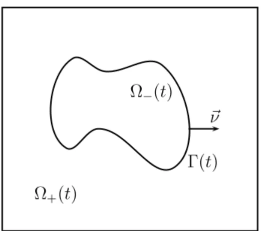
In this section we state the equations governing the evolution of fluidic membranes, as introduced by Arroyo and DeSimone (2009). Let Ω ⊂ Rd be a given domain, where d = 2 or d= 3. We seek a time dependent interface (Γ(t))t∈[0,T], Γ(t)⊂ Ω, which for all t ∈ [0, T] separates Ω into a domain Ω+(t), occupied by the outer phase, and a domain
~ν
Γ(t) Ω−(t)
Ω+(t)
Figure 1: The domain Ω in the case d= 2.
Ω−(t) := Ω\Ω+(t), which is occupied by the inner phase, see Figure 1 for an illustration.
For later use, we assume that (Γ(t))t∈[0,T] is a sufficiently smooth evolving hypersurface without boundary that is parameterized by ~x(·, t) : Υ → Rd, where Υ ⊂ Rd is a given reference manifold, i.e. Γ(t) =~x(Υ, t). Then
V(~z, t) :=~ ~xt(~q, t) ∀ ~z=~x(~q, t)∈Γ(t) (2.1) defines the velocity of Γ(t), andV :=V~ . ~νis the normal velocity of the evolving hypersur- face Γ(t), where~ν(t) is the unit normal on Γ(t) pointing into Ω+(t). Moreover, we define the space-time surface GT :=S
t∈[0,T]Γ(t)× {t}.
Let ρ(t) = ρ+XΩ+(t) +ρ−XΩ−(t), with ρ± ∈ R≥0, denote the fluid densities, where here and throughout XA defines the characteristic function for a set A. Denoting by
~u: Ω×[0, T]→Rd the fluid velocity, by σ : Ω×[0, T]→Rd×d the stress tensor, and by f~: Ω×[0, T]→Rd a possible volume force, the incompressible Navier–Stokes equations in the two phases are given by
ρ(~ut+ (~u .∇)~u)− ∇. σ=ρ ~f in Ω±(t), (2.2a)
∇. ~u= 0 in Ω±(t), (2.2b)
~u=~g on∂1Ω, (2.2c)
σ ~n =~0 on∂2Ω, (2.2d) where ∂Ω =∂1Ω∪∂2Ω, with ∂1Ω∩∂2Ω =∅, denotes the boundary of Ω with outer unit normal~n. Hence (2.2c) prescribes a possibly inhomogeneous Dirichlet condition for the velocity on ∂1Ω, which collapses to the standard no-slip condition when ~g = ~0, while (2.2d) prescribes a stress-free condition on ∂2Ω. Throughout this paper we assume that Hd−1(∂1Ω) > 0. We will also assume w.l.o.g. that ~g is extended so that~g : Ω → Rd. In addition, the stress tensor in (2.2a) is defined by
σ=µ(∇~u+ (∇~u)T)−pId = 2µ D(~u)−pId, , (2.3)
where Id∈Rd×d denotes the identity matrix andD(~u) := 12(∇~u+ (∇~u)T) is the rate-of- deformation tensor, with ∇~u= ∂xjui
d
i,j=1. Moreover, p: Ω×[0, T]→Ris the pressure and µ(t) =µ+XΩ+(t)+µ−XΩ−(t), with µ± ∈R>0, denotes the dynamic viscosities in the two phases. On the free surface Γ(t), the following conditions need to hold:
[~u]+− =~0 on Γ(t), (2.4a)
ρΓ∂t•~u− ∇s. σΓ = [σ ~ν]+−+α ~fΓ on Γ(t), (2.4b)
∇s. ~u= 0 on Γ(t), (2.4c)
V~. ~ν =~u . ~ν on Γ(t), (2.4d)
whereρΓ ∈R≥0 denotes the surface material density, α∈R>0 is the bending rigidity and f~Γ := fΓ~ν is defined by (1.1). In addition, ∇s. denotes the surface divergence on Γ(t), and the surface stress tensor is given by
σΓ= 2µΓDs(~u)−pΓPΓ on Γ(t), (2.5) where µΓ ∈ R>0 is the interfacial shear viscosity and pΓ denotes the surface pressure, which acts as a Lagrange multiplier for the incompressibility condition (2.4c). Here
PΓ= Id−~ν⊗~ν on Γ(t) (2.6a)
and
Ds(~u) = 12PΓ(∇s~u+ (∇s~u)T)PΓ on Γ(t), (2.6b) where ∇s = PΓ∇ = (∂s1, . . . , ∂sd) denotes the surface gradient on Γ(t), and ∇s~u =
∂sjui
d
i,j=1. Moreover, as usual, [~u]+− := ~u+−~u− and [σ ~ν]+− := σ+~ν−σ−~ν denote the jumps in velocity and normal stress across the interface Γ(t). Here and throughout, we employ the shorthand notation~b± :=~b |Ω±(t) for a function ~b : Ω× [0, T] → Rd; and similarly for scalar and matrix-valued functions. In addition,
∂t•ζ =ζt+~u .∇ζ ∀ ζ ∈H1(GT) (2.7) denotes the material time derivative of ζ on Γ(t). We compute ∂t•ζ with the help of an extension of ζ to a neighborhood of GT. Here we stress that the derivative in (2.7) is well-defined, and depends only on the values of ζ on GT, even though ζt and ∇ζ do not make sense separately for a function defined on GT; see e.g. Dziuk and Elliott (2013, p.
324). The system (2.2a–d), (2.3), (2.4a–d), (2.5) is closed with the initial conditions Γ(0) = Γ0, ρ ~u(·,0) =ρ ~u0 in Ω, ρΓ~u(·,0) =ρΓ~u0 on Γ0, (2.8) where Γ0 ⊂ Ω and ~u0 : Ω → Rd are given initial data satisfying ρ∇. ~u0 = 0 in Ω, ρΓ∇s. ~u0 = 0 on Γ0 and ρ+~u0 = ρ+~g on ∂1Ω. Of course, in the case ρ− =ρ+ =ρΓ = 0 the initial data~u0 is not needed. Similarly, in the case ρ−=ρ+= 0 andρΓ >0 the initial data~u0 is only needed on Γ0. However, for ease of exposition, and in view of the unfitted nature of our numerical method, we will always assume that ~u0, if required, is given on all of Ω.
It is not difficult to show that the conditions (2.2b) enforce volume preservation for the phases, while (2.4c) leads to the conservation of the total surface area Hd−1(Γ(t)), see Section 3 below for the relevant proofs. As an immediate consequence we obtain that spheres remain spheres, and that spheres with a zero bulk velocity are stationary solutions.
Furthermore, we note that
∇s. σΓ= 2µΓ∇s. Ds(~u)− ∇s.[pΓPΓ] = 2µΓ∇s. Ds(~u)− ∇spΓ−κpΓ~ν . (2.9) Here κ denotes the mean curvature of Γ(t), i.e. the sum of the principal curvatures κi, i = 1, . . . , d−1, of Γ(t), where we have adopted the sign convention that κ is negative where Ω−(t) is locally convex. In particular, it holds that
∆sid =~ κ~ν =:~κ on Γ(t), (2.10) where ∆s =∇s.∇s is the Laplace–Beltrami operator on Γ(t).
Assuming there are two solutions {(Γ(t), ~u(·, t), p(i)(·, t), p(i)Γ (·, t))}t∈[0,T], i = 1,2, to the problem (2.2a–d), (2.3), (2.4a–d), (2.5) and (2.8), then it follows from (2.3) and (2.9) that
∇p¯±=~0 in Ω±(t), (2.11a)
∇sp¯Γ+κp¯Γ~ν = [¯p ~ν]+− on Γ(t), (2.11b) where ¯p=p(1)−p(2) and ¯pΓ =p(1)Γ −p(2)Γ . Therefore ¯p± is constant on Ω±(t). In addition, since∇sp¯Γ is tangential, we obtain that∇sp¯Γ =~0, and hence ¯pΓ is a constant. Moreover, (2.11b) implies that κp¯Γ = ¯p+−p¯−. So if κ is not constant, which is the case if Γ(t) is not a sphere, then ¯pΓ = 0 and ¯p+ = ¯p−. Hence pΓ in this case is unique, and p is unique in Ω up to an additive constant. If κ is constant, however, i.e. if Γ(t) is a sphere, thenpΓ is only unique up to an additive constant, which is fixed by the two additive constants in the bulk phases. For more details see the discussion around (3.13) below.
Finally, we recall that the source term f~Γ =fΓ~ν in (2.4b), with fΓ defined in (1.1), is the first variation of E(Γ(t)), i.e.
1 2
d
dthκ,κiΓ(t) =− hfΓ,ViΓ(t)=−D f~Γ, ~VE
Γ(t) ,
where h·,·iΓ(t) denotes the L2–inner product on Γ(t). It does not appear possible to derive a stable discretization of the system (2.2a–d), (2.3), (2.4a–d), (2.5) based on the formulation (1.1). Hence in this paper we will make use of the stable approximation of Willmore flow introduced in Dziuk (2008), which is based on a discretization of the curvature vector κ~ =κ~ν, and on the identity
1 2
d
dth~κ, ~κiΓ(t) =−D
∇s~κ,∇sV~E
Γ(t)−D
∇s. ~κ,∇s. ~VE
Γ(t)−12 D
|~κ|2∇sid,~ ∇sV~E
Γ(t)
+ 2D
∇sκ~, Ds(V)~ ∇sid~E
Γ(t). (2.12)
3 Weak formulation
Before introducing our finite element approximation, we will state an appropriate weak formulation. With this in mind, we introduce the following function spaces for a given
~b∈[H1(Ω)]d:
U(~b) := {~ϕ∈[H1(Ω)]d :ϕ~ =~b on∂1Ω}, V(~b) :=L2(0, T;U(~b))∩H1(0, T; [L2(Ω)]d), VΓ(~b) :={~ϕ∈V(~b) :ϕ~|GT∈[H1(GT)]d}.
In addition, we let P:=L2(Ω) and define b
P:=
({η∈P:R
Ωη dLd= 0} if Hd−1(∂2Ω) = 0, P if Hd−1(∂2Ω) >0.
Letting (·,·) andh·,·i∂2Ω denote the L2–inner products on Ω and∂2Ω, respectively, we recall from Barrettet al. (2014c) that it follows from (2.2a–d) and (2.3) that
(ρ[~ut+ (~u .∇)~u], ~ξ)
= 12 d
dt(ρ ~u, ~ξ) + (ρ ~ut, ~ξ)−(ρ ~u, ~ξt) + (ρ,[(~u .∇)~u]. ~ξ−[(~u .∇)ξ]~ . ~u)
+12 ρ+
D~u . ~n, ~u . ~ξE
∂2Ω ∀ ~ξ∈V(~0) (3.1)
and Z
Ω+(t)∪Ω−(t)
(∇. σ). ~ξdLd=−2 (µ D(~u), D(~ξ)) + (p,∇. ~ξ)−D
[σ ~ν]+−, ~ξE
Γ(t) ∀ ξ~∈U(~0), (3.2) where we have also noted for symmetric matrices A∈Rd×d that A :B =A: 12(B+BT) for allB ∈Rd×d. Only slip or free-slip conditions were considered in Barrettet al.(2014c), and so the boundary integral over ∂2Ω did not appear there. But it is easily established that the more general (3.1) also holds, on noting Barrett et al. (2014c, (3.2)).
Similarly to (2.7) we define the following time derivative that follows the parameteri- zation~x(·, t) of Γ(t), rather than ~u. In particular, we let
∂t◦ζ =ζt+V~ .∇ζ ∀ζ ∈H1(GT) ; (3.3) where we stress once again that this definition is well-defined, even though ζt and ∇ζ do not make sense separately for a function ζ ∈ H1(GT). On recalling (2.7) we obtain that
∂t◦ =∂t• if V~ =~u on Γ(t). Moreover, for later use we note that
hζ,∇s. ~ηiΓ(t)+h∇sζ, ~ηiΓ(t) =−hζ ~η, ~κiΓ(t) ∀ζ ∈H1(Γ(t)), ~η ∈[H1(Γ(t))]d (3.4)
and d
dthχ, ζiΓ(t) =h∂t◦χ, ζiΓ(t)+hχ, ∂t◦ζiΓ(t)+D
χ ζ,∇s. ~VE
Γ(t) ∀χ, ζ ∈H1(GT), (3.5) see Definition 2.11 and Lemma 5.2 in Dziuk and Elliott (2013), respectively.
The most natural weak formulation of the system (2.2a–d), (2.3), (2.4a–d), (2.5) uses the fluidic tangential velocity for the evolution of Γ(t), and so (2.4d) is replaced byV~ =~u on Γ(t). It then follows from (2.4b), (2.9), and (3.4) that
ρΓ
D∂t•~u, ~ξE
Γ(t)+ 2µΓ
DDs(~u), Ds(~ξ)E
Γ(t)−D
pΓ,∇s. ~ξE
Γ(t)
=D
[σ ~ν]+−, ~ξE
Γ(t)+αD f~Γ, ~ξE
Γ(t) ∀ξ~∈H1(GT), (3.6) where we have noted for symmetric matrices A ∈ Rd×d that PΓAPΓ : B = PΓAPΓ :
1
2PΓ(B + BT)PΓ for all B ∈ Rd×d. This weak formulation of the system (2.2a–d), (2.3), (2.4a–d), (2.5) is then given as follows. Find Γ(t) = ~x(Υ, t) for t ∈ [0, T] with V ∈~ [L2(GT)]d, and functions~u ∈VΓ(~g), p∈L2(0, T;bP), pΓ∈L2(GT),κ~ ∈[H1(GT)]d and f~Γ∈[L2(GT)]d such that for almost all t∈(0, T) it holds that
1 2
d
dt(ρ ~u, ~ξ) + (ρ ~ut, ~ξ)−(ρ ~u, ~ξt) + (ρ,[(~u .∇)~u]. ~ξ−[(~u .∇)ξ]~ . ~u) +ρ+
D~u . ~n, ~u . ~ξE
∂2Ω
+ 2 (µ D(~u), D(~ξ))−(p,∇. ~ξ) +ρΓD
∂t◦~u, ~ξE
Γ(t)+ 2µΓD
Ds(~u), Ds(~ξ)E
Γ(t)
−D
pΓ,∇s. ~ξE
Γ(t) = (ρ ~f , ~ξ) +αD f~Γ, ~ξE
Γ(t) ∀ξ~∈VΓ(~0), (3.7a)
(∇. ~u, ϕ) = 0 ∀ϕ ∈bP, (3.7b)
h∇s. ~u, ηiΓ(t) = 0 ∀ η∈L2(Γ(t)), (3.7c)
DV −~ ~u, ~χE
Γ(t) = 0 ∀ χ~ ∈[L2(Γ(t))]d, (3.7d)
h~κ, ~ηiΓ(t)+D
∇sid,~ ∇s~ηE
Γ(t)= 0 ∀ ~η∈[H1(Γ(t))]d, (3.7e)
Df~Γ, ~χE
Γ(t)=h∇sκ~,∇s~χiΓ(t)+h∇s. ~κ,∇s. ~χiΓ(t)+12D
|~κ|2∇sid,~ ∇sχ~E
Γ(t)
−2D
∇sκ~, Ds(~χ)∇sid~E
Γ(t) ∀ χ~ ∈[H1(Γ(t))]d, (3.7f) as well as the initial conditions (2.8), where in (3.7d) we have recalled (2.1). Here (3.7a–e) can be derived analogously to the weak formulation presented in Barrett et al.(2014c,a), recall (3.1), (3.2), (3.6) and (2.10). In addition, (3.7f) is based on (2.12).
In what follows we would like to derive an energy bound for a solution of (3.7a–f), where for ease of exposition we consider only the case~g=~0. All of the following considerations are formal, in the sense that we make the appropriate assumptions about the existence, boundedness and regularity of a solution to (3.7a–f). Firstly, it follows from (3.5), (3.7d)
and (3.7c) with η=|~u|Γ(t) |2 that
1 2ρΓ d
dth~u, ~uiΓ(t) = 12ρΓ
∂t◦|~u|2,1
Γ(t)+12 ρΓD
∇s. ~V,|~u|2E
Γ(t)
=ρΓh∂t◦~u, ~uiΓ(t)+ 12ρΓ
∇s. ~u,|~u|2
Γ(t) =ρΓh∂t◦~u, ~uiΓ(t). (3.8) Now choosing ξ~=~u in (3.7a), recall that~g =~0, ϕ = p(·, t) in (3.7b) and η = pΓ(·, t) in (3.7c) yields, on combining with (3.8), that
1 2
d dt
kρ12 ~uk20+ρΓh~u, ~uiΓ(t)
+ 2kµ12 D(~u)k20+ 2µΓ
Ds(~u), Ds(~u)
Γ(t)
+ 12ρ+
~u . ~n,|~u|2
∂2Ω = (ρ ~f , ~u) +αD f~Γ, ~uE
Γ(t). (3.9)
Combining (3.9) with (2.12), on choosing χ~ = f~Γ in (3.7d) and χ~ = V~ in (3.7f), yields that
1 2
d dt
kρ12 ~uk20+ρΓh~u, ~uiΓ(t)+αh~κ, ~κiΓ(t)
+ 2kµ12 D(~u)k20+ 2µΓ
Ds(~u), Ds(~u)
Γ(t)
+ 12ρ+
~u . ~n,|~u|2
∂2Ω = (ρ ~f , ~u). (3.10)
Moreover, we note that it immediately follows from (3.5) and (3.7c,d) that d
dtHd−1(Γ(t)) = d
dth1,1iΓ(t) =D
1,∇s. ~VE
Γ(t) =h1,∇s. ~uiΓ(t) = 0. (3.11) In addition, the volume of Ω−(t) is preserved in time, i.e. the mass of each phase is conserved. To see this, choose ~χ =~ν in (3.7d) and ϕ = (XΩ−(t)− LdL(Ωd(Ω)−(t))) in (3.7b) to obtain
d
dtLd(Ω−(t)) = D V, ~ν~ E
Γ(t) =h~u, ~νiΓ(t) = Z
Ω−(t)
∇. ~udLd= 0. (3.12) Recalling the argument on the uniqueness of the pressures p and pΓ below (2.11a,b), we note the following LBB-type condition, provided that Γ(t) is not a sphere:
(ϕ,η)∈bPinf×L2(Γ(t))
sup
~ξ∈UΓ(~0)
(ϕ,∇. ~ξ) +D
η,∇s. ~ξE
Γ(t)
(kϕk0+kηk0,Γ(t)) (k~ξk1+kPΓξ~|Γ(t) k1,Γ(t)) ≥C > 0. (3.13) Here we have defined the space UΓ(~0) := {~ξ ∈ U(~0) : PΓξ~|Γ(t)∈H1(Γ(t))}. In addition, kηk20,Γ(t) := hη, ηiΓ(t) and k~ηk21,Γ(t) := h~η, ~ηiΓ(t) +h∇s~η,∇s~ηiΓ(t) for ~η ∈ H1(Γ(t)) This can be deduced from the pressure reconstruction result in Lengeler (2014) in the case
∂1Ω = ∂Ω.
4 Semidiscrete finite element approximation
For simplicity we consider Ω to be a polyhedral domain. Then let Th be a regular partitioning of Ω into disjoint open simplices ohj, j = 1, . . . , JΩh. Associated with Th are the finite element spaces
Skh :={χ∈C(Ω) :χ|o∈ Pk(o) ∀ o∈ Th} ⊂H1(Ω), k∈N,
where Pk(o) denotes the space of polynomials of degree k on o. We also introduce S0h, the space of piecewise constant functions on Th. Let {ϕhk,j}Kj=1kh be the standard basis functions for Skh, k ≥ 0. We introduce I~kh : [C(Ω)]d → [Skh]d, k ≥ 1, the standard interpolation operators, such that (I~kh~η)(~phk,j) =~η(~phk,j) for j = 1, . . . , Kkh; where{~phk,j}Kj=1kh denotes the coordinates of the degrees of freedom ofSkh, k ≥1. In addition we define the standard projection operatorI0h :L1(Ω) →S0h, such that
(I0hη)|o= 1 Ld(o)
Z
o
ηdLd ∀ o∈ Th.
Our approximation to the velocity and pressure on Th will be finite element spaces Uh(~g) ⊂ U(I~kh~g), for some k ≥ 2, and Ph(t) ⊂ P. For the former we assume from now on that ~g ∈ [C(Ω)]d, while for the latter we assume that S1h ⊂ Ph(t). We require also the space Pbh(t) := Ph(t)∩Pb. For the finite element spaces (Uh,Ph) we may choose, for example, the lowest order Taylor–Hood element P2–P1, the P2–P0 element or the P2–(P1+P0) element on setting Uh = [S2h]d ∩U(I~2h~g), and Ph = S1h, S0h or S1h +S0h, respectively. We refer to Barrettet al. (2013, 2014c) for more details.
For the numerical approximation of the evolution of fluidic membranes it is desirable to maintain the surface area of the interface, recall (3.11), as well as the volume of the two phases, recall (3.12). In Barrett et al.(2013, 2014c) the present authors augmented the pressure space by the characteristic function of the inner phase in order to obtain discretizations that maintain the volume of the two phases. This enrichment of the pres- sure space is an example of an XFEM approach, and we refer to this particular approach as XFEMΓ. Unfortunately, it does not appear possible to prove a discrete analogue of (3.11) for the XFEMΓ approach from Barrett et al. (2013, 2014c). Hence in this paper we will modify the XFEMΓ approach so that we obtain numerical approximations that satisfy discrete analogues of both (3.12) and (3.11). From a practical point of view, this approach is very close to the procedure in Barrettet al.(2013, 2014c). But the introduced modifications mean that the adjustments to the finite element approximations no longer have an interpretation within the XFEM framework. However, the new approach may be interpreted as an example of the recently proposed virtual element method, see below for further details.
The parametric finite element spaces in order to approximate e.g.~κandpΓare defined as follows, see also Barrett et al. (2008a). Let Γh(t) ⊂ Rd be a (d − 1)-dimensional polyhedral surface, i.e. a union of non-degenerate (d−1)-simplices with no hanging vertices (see Deckelnick et al.(2005, p. 164) for d= 3), approximating the closed surface Γ(t). In
particular, let Γh(t) =SJΓ
j=1σjh(t), where {σjh(t)}Jj=1Γ is a family of mutually disjoint open (d−1)-simplices with vertices {~qkh(t)}Kk=1Γ . Then let
V(Γh(t)) := {~χ∈[C(Γh(t))]d:~χ|σh
j is linear ∀j = 1, . . . , JΓ}
=: [W(Γh(t))]d⊂[H1(Γh(t))]d,
where W(Γh(t))⊂ H1(Γh(t)) is the space of scalar continuous piecewise linear functions on Γh(t), with{χhk(·, t)}Kk=1Γ denoting the standard basis of W(Γh(t)), i.e.
χhk(~qhl(t), t) =δkl ∀k, l∈ {1, . . . , KΓ}, t∈[0, T]. (4.1) For later purposes, we also introduce πh(t) : C(Γh(t)) → W(Γh(t)), the standard inter- polation operator at the nodes {~qkh(t)}Kk=1Γ , and similarly ~πh(t) : [C(Γh(t))]d → V(Γh(t)).
For scalar and vector functions η, ζ on Γh(t) we introduce the L2–inner product h·,·iΓh(t) over the polyhedral surface Γh(t) as follows
hη, ζiΓh(t) :=
Z
Γh(t)
η . ζ dHd−1.
If v, w are piecewise continuous, with possible jumps across the edges of {σjh}Jj=1Γ , we introduce the mass lumped inner product h·,·ihΓh(t) as
hη, ζihΓh(t) := 1d
JΓ
X
j=1
Hd−1(σjh) Xd k=1
(η . ζ)((~qjhk)−),
where {~qhjk}dk=1 are the vertices of σjh, and where we define η((~qhjk)−) := lim
σjh∋~p→~qjkh η(~p).
Following Dziuk and Elliott (2013, (5.23)), we define the discrete material velocity for
~z∈Γh(t) by
V~h(~z, t) :=
KΓ
X
k=1
d dt~qkh(t)
χhk(~z, t). (4.2)
Then, similarly to (3.3), we define
∂◦,ht ζ =ζt+V~h.∇ζ ∀ ζ ∈H1(GTh), where GTh := [
t∈[0,T]
Γh(t)× {t}. (4.3) For later use, we also introduce the finite element spaces
W(GTh) := {χ∈C(GTh) :χ(·, t)∈W(Γh(t)) ∀ t ∈[0, T]}, WT(GTh) := {χ∈W(GTh) :∂t◦,hχ∈C(GTh)},
as well as Vh
Γh(~g) :={φ~∈H1(0, T;Uh(~g)) :~χ∈[WT(GT)]d, where ~χ(·, t) =~πh[φ~|Γh(t)] ∀ t∈[0, T]}.
On differentiating (4.1) with respect to t, it immediately follows that
∂t◦,hχhk = 0 ∀k ∈ {1, . . . , KΓ}, (4.4) see Dziuk and Elliott (2013, Lem. 5.5). It follows directly from (4.4) that
∂t◦,hζ(·, t) =
KΓ
X
k=1
χhk(·, t) d
dtζk(t) on Γh(t) for ζ(·, t) =PKΓ
k=1ζk(t)χhk(·, t)∈W(Γh(t)), and hence ∂t◦,hid =~ V~h on Γh(t).
We recall from Dziuk and Elliott (2013, Lem. 5.6) that d
dt Z
σjh(t)
ζ dHd−1 = Z
σjh(t)
∂t◦,hζ+ζ∇s. ~Vh dHd−1 ∀ ζ ∈H1(σh(t)), j ∈ {1, . . . , JΓ}, (4.5) which immediately implies that
d
dthη, ζiΓh(t) =h∂t◦,hη, ζiΓh(t)+hη, ∂t◦,hζiΓh(t)+hη ζ,∇s. ~VhiΓh(t) ∀ η, ζ ∈WT(GTh). (4.6) Similarly, we recall from Barrettet al. (2014a, Lem. 2.1) that
d
dthη, ζihΓh(t) =h∂t◦,hη, ζihΓh(t)+hη, ∂◦,ht ζihΓh(t)+hη ζ,∇s. ~VhihΓh(t) ∀η, ζ ∈WT(GTh). (4.7) Similarly to (2.6a,b), we introduce
PΓh = Id−~νh⊗~νh on Γh(t), (4.8a) and
Dhs(~η) = 12PΓh(∇s~η+ (∇s~η)T)PΓh on Γh(t), (4.8b) where here ∇s=PΓh∇ denotes the surface gradient on Γh(t).
Given Γh(t), we let Ωh+(t) denote the exterior of Γh(t) and let Ωh−(t) denote the interior of Γh(t), so that Γh(t) =∂Ωh−(t) = Ωh−(t)∩Ωh+(t). We then partition the elements of the bulk mesh Th into interior, exterior and interfacial elements as follows. Let
T−h(t) :={o ∈ Th :o⊂Ωh−(t)}, T+h(t) :={o ∈ Th :o⊂Ωh+(t)}, TΓhh(t) :={o ∈ Th :o∩Γh(t)6=∅}.
Clearly Th = T−h(t)∪ T+h(t)∪ TΓh(t) is a disjoint partition. In addition, we define the piecewise constant unit normal~νh(t) to Γh(t) such that~νh(t) points into Ωh+(t). Moreover, we introduce the discrete density ρh(t)∈S0h and the discrete viscosity µh(t)∈S0h as
ρh(t)|o=
ρ− o∈ T−h(t), ρ+ o∈ T+h(t),
1
2 (ρ−+ρ+) o∈ TΓhh(t),
and µh(t)|o=
µ− o ∈ T−h(t), µ+ o ∈ T+h(t),
1
2(µ−+µ+) o ∈ TΓhh(t).
In what follows we will introduce a finite element approximation for the free boundary problem (2.2a–d), (2.3), (2.4a–d), (2.5). Here U~h(·, t)∈ Uh(~g) will be an approximation to~u(·, t), while Ph(·, t)∈Pbh(t) approximatesp(·, t) andPΓh(·, t)∈W(Γh(t)) approximates pΓ(·, t). When designing such a finite element approximation, a careful decision has to be made about the discrete tangential velocity of Γh(t). The most natural choice is to select the velocity of the fluid, i.e. (3.7d) is appropriately discretized, and that is the approach we adopt in this paper. Overall, we then obtain the following semidiscrete continuous-in-time finite element approximation, which is the semidiscrete analogue of the weak formulation (3.7a–f).
Given Γh(0) andU~h(·,0)∈Uh(~g), find Γh(t) such thatid~ |Γh(t)∈V(Γh(t)) fort∈[0, T], and functions U~h ∈ Vh
Γh(~g), Ph ∈ PhT := {ϕ ∈ L2(0, T;bP) : ϕ(t) ∈ Pbh(t) for a.e. t ∈ (0, T)},PΓh ∈W(GTh),~κh ∈[W(GTh)]dandF~Γh ∈[W(GTh)]dsuch that for almost allt∈(0, T) it holds that
1 2
d dt
ρhU~h, ~ξ +
ρhU~th, ~ξ
−(ρhU~h, ~ξt) +ρ+
DU~h. ~n, ~Uh. ~ξE
∂2Ω
+ 2
µhD(U~h), D(ξ)~ + 12
ρh,[(U~h.∇)U~h]. ~ξ−[(U~h.∇)ξ]~ . ~Uh
−
Ph,∇. ~ξ +ρΓ
D∂t◦,h~πhU~h, ~ξEh
Γh(t)+ 2µΓ
DDhs(~πhU~h), Dhs(~πhξ)~ E
Γh(t)
−D
PΓh,∇s.(~πh~ξ)E
Γh(t) =
ρhf~h, ~ξ +αD
F~Γh, ~ξEh
Γh(t) ∀ ~ξ ∈H1(0, T;Uh(~0)), (4.9a) ∇. ~Uh, ϕ
= 0 ∀ ϕ∈Pbh(t), (4.9b)
D∇s.(~πhU~h), ηE
Γh(t) = 0 ∀η ∈W(Γh(t)), (4.9c)
DV~h, ~χEh
Γh(t) =D
U~h, ~χEh
Γh(t) ∀χ~ ∈V(Γh(t)), (4.9d)
~κh, ~η(h) Γh(t)+D
∇sid,~ ∇s~ηE
Γh(t)= 0 ∀ ~η∈V(Γh(t)), (4.9e) DF~Γh, ~χEh
Γh(t) =
∇s~κh,∇sχ~
Γh(t)+
∇s. ~κh,∇s. ~χ
Γh(t)+12D
|~κh|2∇sid,~ ∇s~χE(h) Γh(t)
−2D
∇s~κh, Dhs(~χ)∇sid~E
Γh(t) ∀ χ~ ∈V(Γh(t)), (4.9f) where we recall (4.2). Here we have defined f~h(·, t) :=I~2hf~(·, t), where here and through- out we assume that f~ ∈ L2(0, T; [C(Ω)]d). We observe that (4.9d) collapses to V~h =
~πhU~h |Γh(t)∈ V(Γh(t)), which on recalling (4.3) turns out to be crucial for the stability analysis for (4.9a–f). It is for this reason that we use mass lumping in (4.9d). The su- perscript ·(h) in (4.9e,f) means that we can consider the corresponding terms either with or without mass lumping. Here we note that the scheme (4.9d–f), with true integration used throughout, and with U~h in (4.9d) replaced by F~h, is the stable approximation of Willmore flow from Dziuk (2008), see also Deckelnick and Dziuk (2009) for the cased= 2.
In fact, for d= 2 we observe that ∇s~κh,∇sχ~
Γh(t)+
∇s. ~κh,∇s. ~χ
Γh(t)−2D
∇s~κh, Dhs(~χ)∇sid~E
Γh(t)
=
∇s~κh,∇s~χ
Γh(t)−
∇s. ~κh,∇s. ~χ
Γh(t)=
~κhs. ~νh, ~χs. ~νh
Γh(t),
where ·s denotes differentiation with respect to arclength; compare also Barrett et al.
(2012, (3.12a,b)).
In the following theorem we derive discrete analogues of (3.10) and (3.11) for the scheme (4.9a–f).
Theorem. 4.1. Let {(Γh, ~Uh, Ph, PΓh, ~κh, ~FΓh)(t)}t∈[0,T] be a solution to (4.9a–f). Then, in the case~g =~0, it holds that
1 2
d dt
k[ρh]12 U~hk20+ρΓ
DU~h, ~UhEh
Γh(t)+α
~κh, ~κh(h) Γh(t)
+ 2k[µh]12 D(U~h)k20 + 2µΓ
DDhs(~πhU~h), Dhs(~πhU~h)E
Γh(t)+12 ρ+
DU~h. ~n,|U~h|2E
∂2Ω = (ρhf~h, ~Uh). (4.10) Moreover, it holds that
d dt
χhk,1
Γh(t) = 0 ∀ k ∈ {1, . . . , KΓ} (4.11) and hence that
d
dtHd−1(Γh(t)) = 0. (4.12)
Proof. Choosing ξ~=U~h in (4.9a), recall that~g =~0, ϕ =Ph in (4.9b) and η=PΓh in (4.9c) yields that
1 2
d
dtk[ρh]12 U~hk20+ 2k[µh]12 D(U~h)k20+ρΓD
∂t◦,h~πhU~h, ~UhEh
Γh(t)+12 ρ+D
U~h. ~n,|U~h|2E
∂2Ω
+ 2µΓ
DDhs(~πhU~h), Dhs(~πhU~h)E
Γh(t) = (ρhf~h, ~Uh) +αD
F~Γh, ~UhEh
Γh(t). (4.13) Moreover, similarly to (3.8), we note that (4.7), (4.9d) and (4.9c) with η = πh[|U~h|Γh(t) |2] imply that
1 2ρΓ
d dt
DU~h, ~UhEh
Γh(t) = 12ρΓ
D∂t◦,h~πh[|U~h|2],1Eh
Γh(t)+ 12ρΓ
D∇s. ~Vh,|U~h|2Eh Γh(t)
=ρΓD
∂t◦,h~πhU~h, ~UhEh
Γh(t)+12ρΓD
∇s.(~πhU~h),|U~h|2Eh
Γh(t)
=ρΓ
D∂t◦,h~πhU~h, ~UhEh
Γh(t). (4.14)
Similarly to (2.12), it is possible to show that
1 2
d dt
~κh, ~κh(h)
Γh(t)=−D
∇s~κh,∇sV~hE
Γh(t)−D
∇s. ~κh,∇s. ~VhE
Γh(t)
− 12D
|~κh|2∇sid,~ ∇sV~hE(h)
Γh(t)+ 2D
∇s~κh, Dhs(V~h)∇sid~E
Γh(t), see Dziuk (2008). Hence choosing χ~ =F~Γh in (4.9d) and χ~ =V~h in (4.9f) yields that
DF~Γh, ~UhEh
Γh(t)=D
F~Γh, ~VhEh
Γh(t) =−12 d dt
~κh, ~κh(h)
Γh(t). (4.15) The desired result (4.10) now directly follows from combining (4.13), (4.14) and (4.15).
Similarly to (3.11), it immediately follows from (4.6) and (4.4), on choosing η=χhk in (4.9c), and on recalling from (4.9d) that V~h =~πhU~h, that
d dt
χhk,1
Γh(t) =D
χhk,∇s. ~VhE
Γh(t) = 0, (4.16)
which proves the desired result (4.11). Summing (4.11) for all k = 1, . . . , KΓ then yields the desired result (4.12).
Remark. 4.2. We remark that (4.11) ensures that the area of the support of each basis function on Γh(t) is conserved. In the cased= 2, and forJΓ being odd, this is equivalent to each element σhj maintaining its length. In particular, if Γh(0) is equidistributed, then Γh(t) will remain equidistributed throughout.
The same result, for arbitrary JΓ ≥ 2 and for d = 2 and d = 3, can be obtained on replacing the space of continuous piecewise linear finite elements W(Γh(t))for the surface pressure functions PΓh, and for the test functions in (4.9c), with the space of discontinuous piecewise constant functions. Then (4.5), similarly to (4.16), immediately yields that
d
dtHd−1(σhj(t)) = 0 ∀ j ∈ {1, . . . , JΓ}. (4.17) While this property may appear desirable at first, our numerical experience for the fully discrete variant of this modified (4.9a–f) indicates that in the case d = 3 the constraint (4.17) is too severe. Here we note that for typical triangulations of Γh(t) it holds that JΓ≈2KΓ. It is for this reason that we prefer the scheme (4.9a–f) as stated.
We observe that it does not appear possible to prove a discrete analogue of (3.12) for the scheme (4.9a–f). The reason is that χ~ = ~νh is not a valid test function in (4.9d).
However, a procedure similarly to the XFEMΓ approach introduced by the authors in Barrett et al. (2013, 2014c) ensures that a modified variant of (4.9a–f) conserves the enclosed volumes. To this end, we introduce the vertex normal function~ωh(·, t)∈V(Γh(t)) with
~ωh(~qhk(t), t) := 1 Hd−1(Λhk(t))
X
j∈Θhk
Hd−1(σjh(t))~νjh|σh
j(t),


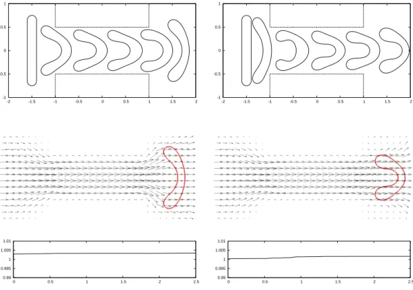
![Figure 5: Flow for a smooth letter “C” for ρ Γ = 0. The plots show the interface Γ m , together with the discrete velocity U~ m on [−1, 1]× [−0.5, 0.5], at times t = 0, 0.05, 0.1, 1.](https://thumb-eu.123doks.com/thumbv2/1library_info/5624410.1692377/32.892.143.759.225.878/figure-flow-smooth-letter-plots-interface-discrete-velocity.webp)
![Figure 6: Flow for a smooth letter “C” for ρ Γ = 1. The plots show the inter- inter-face Γ m , together with the discrete velocity U~ m on [−1, 1] × [−0.5, 0.5], at times t = 0, 0.05, 0.1, 0.3, 0.6, 1](https://thumb-eu.123doks.com/thumbv2/1library_info/5624410.1692377/33.892.144.755.139.1023/figure-flow-smooth-letter-plots-inter-discrete-velocity.webp)