Universit¨ at Regensburg Mathematik
Numerical computations of the dynamics of fluidic membranes and vesicles
John W. Barrett, Harald Garcke and Robert N¨ urnberg
Preprint Nr. 05/2015
John W. Barrett
Department of Mathematics, Imperial College London, London SW7 2AZ, UK Harald Garcke∗
Fakult¨at f¨ur Mathematik, Universit¨at Regensburg, 93040 Regensburg, Germany Robert N¨urnberg
Department of Mathematics, Imperial College London, London SW7 2AZ, UK
Vesicles and many biological membranes are made of two monolayers of lipid molecules and form closed lipid bilayers. The dynamical behaviour of vesicles is very complex and a variety of forms and shapes appear. Lipid bilayers can be considered as a surface fluid and hence the governing equations for the evolution include the surface (Navier–)Stokes equations, which in particular take the membrane viscosity into account. The evolution is driven by forces stemming from the cur- vature elasticity of the membrane. In addition, the surface fluid equations are coupled to bulk (Navier–)Stokes equations.
We introduce a parametric finite element method to solve this complex free boundary problem, and present the first three dimensional numerical computations based on the full (Navier–)Stokes system for several different scenarios. For example, the effects of the membrane viscosity, spontaneous curvature and area difference elasticity (ADE) are studied. In particular, it turns out, that even in the case of no viscosity contrast between the bulk fluids, the tank treading to tumbling transition can be obtained by increasing the membrane viscosity. In addition, we study the tank treading, tumbling and trembling behaviour for different spontaneous curvatures. We also study how features of equilibrium shapes in the ADE and spontaneous curvature models, like budding behaviour or starfish forms, behave in a shear flow.
PACS numbers: 87.16.dm, 87.16.ad, 87.16.dj
I. INTRODUCTION
Lipid membranes consist of a bilayer of molecules, which have a hydrophilic head and two hydrophobic chains. These bilayers typically spontaneously form closed bag-like structures, which are called vesicles. It is observed that vesicles can attain a huge variety of shapes and some of them are similar to the biconcave shape of red blood cells. Since membranes play a fundamental role in many living systems, the study of vesicles is a very ac- tive research field in different scientific disciplines, see e.g. [1–4]. It is the goal of this paper to present a numer- ical approach to study the evolution of lipid membranes.
We present several computations showing quite different shapes, and the influence of fluid flow on the membrane evolution.
Since the classical papers of Canham [5] and Helfrich [6], there has been a lot of work with the aim of de- scribing equilibrium membrane shapes with the help of elastic membrane energies. Canham [5] and Helfrich [6]
introduced a bending energy for a non-flat membrane, which is formulated with the help of the curvature of the membrane. In the class of fixed topologies the rele- vant energy density, in the simplest situation, is propor- tional to the square of the mean curvature κ. The re- sulting energy functional is called the Willmore energy.
∗harald.garcke@ur.de
When computing equilibrium membrane shapes one has to take constraints into account. Lipid membranes have a very small compressibility, and hence can safely be mod- elled as locally incompressible. In addition, the presence of certain molecules in the surrounding fluid, for which the membrane is impermeable, leads to an osmotic pres- sure, which results in a constraint for the volume en- closed by the membrane. The minimal energetic model for lipid membranes consists of the Willmore mean cur- vature functional together with enclosed volume and sur- face area constraints. Already this simple model leads to quite different shapes including the biconcave red blood cell shapes, see [1].
Helfrich [6] introduced a variant of the Willmore en- ergy, with the aim of modelling a possible asymmetry of the bilayer membrane. Helfrich [6] studied the functional R(κ −κ)2, where κ is a fixed constant, the so-called spontaneous curvature. It is argued that the origin of the spontaneous curvature is e.g. a different chemical en- vironment on both sides of the membrane. We refer to [7] and [8] for a recent discussion, and for experiments in situations which lead to spontaneous curvature effects due to the chemical structure of the bilayer.
Typically there is yet another asymmetry in the bilayer leading to a signature in the membrane architecture.
This results from the fact that the two membrane layers have a different number of molecules. Since the exchange of molecules between the layers is difficult, an imbalance is conserved during a possible shape change. The total
area difference between the two layers is proportional to M = R
κ. Several models have been proposed, which describe the difference in the total number of molecules in the two layers with the help of the integrated mean curvature. The bilayer coupling model, introduced by Svetina and coworkers [9–11], assumes that the area per lipid molecule is fixed and assumes that there is no ex- change of molecules between the two layers. Hence the total areas of the two layers are fixed, and on assum- ing that the two layers are separated by a fixed distance, one obtains, to the order of this distance, that the area difference can be approximated by the integrated mean curvature, see [9–11]. We note that a spontaneous cur- vature contribution is irrelevant in the bilayer coupling model as this would only add a constant to the energy as the area and integrated mean curvature are fixed.
Miaoet al.[12] noted that in the bilayer coupling model budding always occurs continuously which is inconsistent with experiments. They hence studied a model in which the area of the two layers are not fixed but can expand or compress under stress. Given a relaxed initial area dif- ference ∆A0, the total area difference ∆A, which is pro- portional to the integrated mean curvature, can deviate from ∆A0. However, the total energy now has a contri- bution that is proportional to (∆A−∆A0)2. This term describes the elastic area difference stretching energy, see [1, 12], and hence one has to pay a price energetically to deviate from the relaxed area difference.
It is also possible to combine the area difference elas- ticity model (ADE-model) with a spontaneous curvature assumption, see Miaoet al.[12] and Seifert [1]. However, the resulting energetical model is equivalent to an area difference elasticity model with a modified ∆A0, see [1]
for a more detailed discussion.
It has been shown that the bilayer coupling model (BC- model) and the area difference elasticity model (ADE- model) lead to a multitude of shapes, which also have been observed in experiments with vesicles. Beside oth- ers, the familiar discocyte shapes (including the “shape”
of a red blood cell), stomatocyte shapes, prolate shapes and pear-like shapes have been observed. In addition, the budding of membranes can be described, as well as more exotic shapes, like starfish vesicles. Moreover, higher genus shapes appear as global or local minima of the energies discussed above. We refer to [1, 12–15] for more details on the possible shapes appearing, when minimiz- ing the energies in the ADE- and BC-models.
Configurational changes of vesicles and membranes cannot be described by energetical considerations alone, but have to be modelled with the help of appropriate evo- lution laws. Several authors considered an L2–gradient flow dynamics of the curvature energies discussed above.
Pure Willmore flow has been studied in [16–21], where the last two papers use a phase field formulation of the Willmore problem. Some authors also took other aspects, such as constraints on volume and area [19, 22, 23], as well as a constraint on the integrated mean curvature [19, 20], into account. The effect of different lipid com-
ponents in anL2–gradient flow approach of the curvature energy has been studied in [24–30].
The above mentioned works considered a global con- straint on the surface area. The membrane, however, is locally incompressible and hence a local constraint on the evolution of the membrane molecules should be taken into account. Several authors included the local inexten- sibility constraint by introducing an inhomogeneous La- grange multiplier for this constraint on the membrane.
This approach has been used within the context of dif- ferent modelling and computational strategies such as the level set approach [31–34], the phase field approach [35–
37], the immersed boundary method [38–40], the inter- facial spectral boundary element method [41] and the boundary integral method [42].
The physically most natural way to consider the local incompressibility constraint makes use of the fact that the membrane itself can be considered as an incompress- ible surface fluid. This implies that a surface Navier–
Stokes system has to be solved on the membrane. The resulting set of equations has to take forces stemming from the surrounding fluid and from the membrane elas- ticity into account. In total, bulk Navier–Stokes equa- tions coupled to surface Navier–Stokes equations have to be solved. As the involved Reynolds numbers for vesicles are typically small one can often replace the full Navier–
Stokes equations by the Stokes systems on the surface and in the bulk. The incompressibility condition in the bulk (Navier–)Stokes equations naturally leads to conser- vation of the volume enclosed by the membrane and the incompressibility condition on the surface leads a conser- vation of the membrane’s surface area. A model involving coupled bulk-surface (Navier–)Stokes equations has been proposed by Arroyo and DeSimone [43], and it is this model that we want to study numerically in this paper.
Introducing forces resulting from membrane energies in fluid flow models has been studied numerically before by different authors, [31–33, 36, 37, 40]. However, typi- cally these authors studied simplified models, and either volume or surface constraints were enforced by Lagrange multipliers. In addition, either just the bulk or just the surface (Navier–)Stokes equations have been solved. The only work considering simultaneously bulk and surface Navier–Stokes equations are Arroyoet al. [44] and Bar- rett et al. [45, 46], where the former work is restricted to axisymmetric situations. In the present paper we are going to make use of the numerical method introduced in [45, 46].
The paper is organized as follows. In the next section we precisely state the mathematical model, consisting of the curvature elasticity model together with a cou- pled bulk-surface (Navier–)Stokes system. In Section III we introduce our numerical method which consists of an unfitted parametric finite element method for the mem- brane evolution. The curvature forcing is discretized and coupled to the Navier–Stokes system in a stable way us- ing the finite element method for the fluid unknowns.
Numerical computations in Section IV demonstrate that
we can deal with a variety of different membrane shapes and flow scenarios. In particular, we will study what in- fluence the membrane viscosity, the area difference elas- ticity (ADE) and the spontaneous curvature have on the evolution of bilayer membranes in shear flow. We finish with some conclusions.
II. A CONTINUUM MODEL FOR FLUIDIC MEMBRANES
We consider a continuum model for the evolution of biomembranes and vesicles, which consists of a curvature elasticity model for the membrane and the Navier–Stokes equations in the bulk and on the surface. The model is based on a paper by Arroyo and DeSimone [43], where in addition we also allow the curvature energy model to be an area difference elasticity model. We first introduce the curvature elasticity model and then describe the coupling to the surface and bulk Navier–Stokes equations.
The thickness of the lipid bilayer in a vesicle is typi- cally three to four orders of magnitude smaller than the typical size of the vesicle. Hence the membrane can be modelled as a two dimensional surface Γ in R3. Given the principal curvatures κ1 andκ2 of Γ, one can define the mean curvature
κ=κ1+κ2 and the Gauß curvature
K=κ1κ2
(as often in differential geometry we choose to take the sum of the principal curvatures as the mean curvature, instead of its mean value). The classical works of Can- ham [5] and Helfrich [6] derive a local bending energy, with the help of an expansion in the curvature, and they obtain
Z
Γ
α
2κ2+αGK
ds (1)
as the total energy of a symmetric membrane. The pa- rameters α, αG have the dimension of energy and are called the bending rigidity αand the Gaussian bending rigidityαG. If we consider closed membranes with a fixed topology, the termR
ΓKdsis constant and hence we will neglect the Gaussian curvature term in what follows.
As discussed above, the total area difference ∆Aof the two lipid layers is, to first order, proportional to
M(Γ) = Z
Γ
κds .
Taking now into account that there is an optimal area difference ∆A0, the authors in [47–49] added a term pro- portional to
(M(Γ)−M0)2
to the curvature energy, where M0 is a fixed constant which is proportional to the optimal area difference.
For non-symmetric membranes a certain mean curva- tureκcan be energetically favourable. Then the elastic- ity energy (1) is modified to
Z
Γ
α
2(κ−κ)2+αGK ds .
The constant κ is called spontaneous curvature. Tak- ing into account that R
ΓαGK ds does not change for a evolution within a fixed topology class, the most gen- eral bending energy that we use in this paper is given by α E(Γ) with the dimensionless energy
E(Γ) = 1 2
Z
Γ
(κ−κ)2ds+β
2 (M(Γ)−M0)2, (2) whereβ has the dimension (length1 )2.
We now consider a continuum model for the fluid flow on the membrane and in the bulk, inside and outside of the membrane. We assume that the closed, time dependent membrane (Γ(t))t≥0 lies inside a spatial do- main Ω ⊂ R3. For all times the membrane separates Ω into an inner domain Ω−(t) and an outer domain Ω+(t) = Ω\Ω−(t). Denoting by ~u the fluid velocity and bypthe pressure, the bulk stress tensor is given by σ= 2µ D(~u)−pId, with D(~u) = 12(∇~u+ (∇~u)T) be- ing the bulk rate-of-strain tensor. We assume that the Navier–Stokes system
ρ(~ut+ (~u .∇)~u)− ∇. σ= 0, ∇. ~u= 0
holds in Ω−(t) and Ω+(t). Hereρandµ are the density and dynamic viscosity of the fluid, which can take differ- ent (constant) valuesρ±,µ±in Ω±(t). Arroyo and DeS- imone [43] used the theory of interfacial fluid dynamics, which goes back to Scriven [50], to introduce a relaxation dynamics for fluidic membranes. In this model the fluid velocity is assumed to be continuous across the mem- brane, the membrane is moved in the normal direction with the normal velocity of the bulk fluid and, in addi- tion, the surface Navier–Stokes equations
ρΓ∂t•~u− ∇s. σΓ = [σ]+−~ν+α ~fΓ, ∇s. ~u= 0 have to hold on Γ(t). Here ρΓ is the surface material density,∂t•is the material derivative and∇s,∇s.are the gradient and divergence operators on the surface. The surface stress tensor is given by
σΓ= 2µΓDs(~u)−pΓPΓ,
wherepΓ is the surface pressure,µΓ is the surface shear viscosity,PΓis the projection onto the tangent space and
Ds(~u) = 12PΓ(∇s~u+ (∇s~u)T)PΓ
is the surface rate-of-strain tensor. Furthermore, the term [σ]+−~ν = σ+~ν−σ−~ν is the force exerted by the
bulk on the membrane, where~νdenotes the exterior unit normal to Ω−(t). The remaining term α ~fΓ denotes the forces stemming from the elastic bending energy. These forces are given by the first variation of the bending en- ergyα E(Γ(t)), see [1, 43]. It turns out thatf~Γpoints in the normal direction, i.e. f~Γ =fΓ~ν, and we obtain, see [1, 51],
fΓ=−∆sκ−(κ−κ)|∇s~ν|2+12(κ−κ)2κ
+β(M(Γ)−M0) (|∇s~ν|2−κ2) on Γ(t). (3) Here ∆sis the surface Laplace operator,∇s~νis the Wein- garten map and|∇s~ν|2=κ12+κ22. Assuming e.g. no-slip boundary conditions on ∂Ω, the boundary of Ω, we ob- tain that the total energy can only decrease, i.e.
d dt
Z
Ω
ρ
2|~u|2dx+ρΓ
2 Z
Γ
|~u|2ds+α E(Γ)
=−2 Z
Ω
µ|D(~u)|2dx+µΓ
Z
Γ
|Ds(~u)|2ds
≤0. (4) We now non-dimensionalize the problem. We choose a time scale ˜t, a length scale ˜xand the resulting velocity scale ˜u = ˜x/˜t. Then we define the bulk and surface Reynolds numbers
Re = ˜x ρ+u/µ˜ + and ReΓ= ˜x ρΓu/µ˜ Γ, the bulk and surface pressure scales
˜
p=µ+/˜t and p˜Γ=µ+x/˜ ˜t=µ+u ,˜ and
˜
ρ=ρ/ρ+=
(1 in Ω+
ρ−/ρ+ in Ω−
,
˜
µ=µ/µ+=
(1 in Ω+
µ−/µ+ in Ω−
,
˜
µΓ=µΓ/(µ+x)˜ ,
as well as the new independent variablesxb=x/˜x,bt=t/˜t.
For the unknowns
~b
u=~u/˜u , pb=p/˜p , pbΓ =pΓ/p˜Γ
we now obtain the following set of equations (on dropping the b-notation for the new variables for ease of exposi- tion)
Re ˜ρ(~ut+ (~u .∇)~u)−µ˜∆~u+∇p= 0 in Ω±(t), ReΓµ˜Γ∂t•~u− ∇s. 2 ˜µΓDs(~u)−pΓPΓ
=
2 ˜µ D(~u)−pId+
−~ν+αnewf~Γnew on Γ(t), (5) withf~Γnew=fΓnew~ν,
fΓnew=−∆sκ−(κ−κnew)|∇s~ν|2+12(κ−κnew)2κ +βnew(M(Γ)−M0new) (|∇s~ν|2−κ2),
αnew = α/(µ+u˜x˜2) and κnew = ˜xκ, M0new = M0/˜x, βnew= ˜x2β. We remark that the Reynolds numbers for the two regions in the bulk are given by Re and Re ˜ρ/˜µ, respectively, and that they will in general differ in the case of a viscosity contrast between the inner and outer fluid. In addition to the above equations, we of course also require that ~uhas zero divergence in the bulk and that the surface divergence of~uvanishes on Γ.
Typical values for the bulk dynamic viscosity µ are around 10−3−10−2 kgs m, see [4, 43, 52], whereas the surface shear viscosity typically is about 10−9−10−8 kgs, see [4, 30, 53]. The bending modulus α is typically 10−20 − 10−19 kg ms22, see [30, 52, 53].
The term ˜µΓ=µΓ/(µ+x) in (5) suggests to choose the˜ length scale
˜
x=µΓ/µ+ ⇐⇒ µ˜Γ= 1.
Asαnew=α/(µ+u˜x˜2) =α˜t/(µ+x˜3) appears in (5), we choose the time scale
˜t=µ+x˜3/α . Choosing
µΓ= 5·10−9kg
s , µ+= 10−3kg
s m , α= 10−19kg m2 s2 , see e.g. [43], we obtain the length scale 5·10−6m and the time scale 1.25s, which are typical scales in experiments.
With these scales for length and time together with val- ues of∼103kg/m3for the bulk density and∼10−6kg/m2 for the surface densities, we obtain for the bulk and sur- face Reynolds numbers
Re≈10−5 and ReΓ≈10−8,
and hence we will set the Reynolds numbers to zero in this paper. We note that it is straightforward to also consider positive Reynolds numbers in our numerical al- gorithm, see [45, 46] for details. Together with the other observations above, we then obtain the following reduced set of equations (on dropping the·new superscripts).
−µ˜∆~u+∇p= 0 in Ω±(t),
−2∇s. Ds(~u) +∇s.(pΓPΓ)
=
2 ˜µ D(~u)−pId+
−~ν+α ~fΓ on Γ(t). (6) A downside of the scaling used to obtain (6) is that the surface viscosity no longer appears as an independent pa- rameter. However, studying the effect of the surface vis- cosity, e.g. on the tank treading to tumbling transition in shearing experiments, is one of the main focuses of this paper. It is for this reason that we also consider the following alternative scaling, when suitable length and velocity scales are at hand. For example, we may choose the length scale ˜xbased on the (fixed) size of the mem- brane and a velocity scale ˜ubased on appropriate bound- ary velocity values. In this case we obtain from (5), for
small Reynolds numbers, the following set of equations (on dropping the·newsuperscripts)
−µ˜∆~u+∇p= 0 in Ω±(t),
− ∇s. 2 ˜µΓDs(~u)−pΓPΓ
=
2 ˜µ D(~u)−pId+
−~ν+α ~fΓ on Γ(t). (7) Note that here three non-dimensional parameters remain:
˜
µΓ, ˜µandα. Here ˜µΓ compares the surface shear viscos- ity to the bulk shear viscosity, ˜µis the bulk viscosity ra- tio andαis an inverse capillary number, which describes the ratio of characteristic membrane stresses to viscous stresses. Clearly, the system (6) corresponds to (7) with
˜
µΓ = 1. Hence from now on, we will only consider the scaling (7) in detail.
Of course, the system (7) needs to be supplemented with a boundary condition for~u or σ, and with an ini- tial condition for Γ(0). For the former we partition the boundary ∂Ω of Ω into∂1Ω, where we prescribe a fixed velocity ~u=~g, and ∂2Ω, where we prescribe the stress- free conditionσ ~n =~0, with~n denoting the outer normal to Ω.
III. NUMERICAL APPROXIMATION
The numerical computations in this paper have been performed with a finite element approximation intro- duced by the authors in [45, 46]. The approach discretizes the bulk and surface degrees of freedom independently.
In particular, the surface mesh is not a restriction of the bulk mesh. The bulk degrees of freedoms ~u and p are discretized with the lowest order Taylor–Hood element, P2–P1, in our numerical computations. The evolution of the membrane is tracked with the help of paramet- ric meshes Γh, which are updated by the fluid velocity.
Since the membrane surface is locally incompressible, it turns out that the surface mesh has good mesh proper- ties during the evolution. This is in contrast to other fluid problems with interfaces in which the mesh often deteriorates during the evolution when updated with the fluid velocity, see e.g. [54].
The elastic forcing by the membrane curvature energy, f~Γ, is discretized with the help of a weak formulation by Dziuk [18], which is generalized by Barrettet al. [46] to take spontaneous curvature and area difference elasticity effects into account. A main ingredient of the numerical approach is the fact that one can use a weak formulation of (3) that can be discretized in a stable way. In fact, defining A = β(M(Γ)−M0) and ~y = ~κ+ (A−κ)~ν the following identity, which has to hold for all ~χ on Γ,
characterizesf~Γ: Df~Γ, ~χE
=h∇s~y,∇sχi~ +h∇s. ~y,∇s. ~χi
−2D
∇s~y, Ds(~χ)∇sid~E
+ (A−κ)
~
κ,[∇sχ]~ T~ν
−12D
[|~κ−κ~ν|2−2 (~y . ~κ)]∇sid,~ ∇sχ~E
−AD
(~κ. ~ν)∇sid,~ ∇sχ~E .
Hereh·,·iis theL2–inner product on Γ. Roughly speak- ing the above identity shows that f~Γ has a divergence structure. We remark here that similar divergence struc- tures have been derived with the help of Noether’s theo- rem, see [55, 56].
The numerical method of Barrett et al. [46] has the feature that a semi-discrete, i.e. continuous in time and discrete in space, version of the method obeys a discrete analog of the energy inequality (4). In addition, this semi-discrete version has the property that the volume enclosed by the vesicle and the membrane’s surface area are conserved exactly. After discretization in time these properties are approximately fulfilled to a high accuracy, see Section IV. The fully discrete system is linear and fully coupled in the unknowns. The overall system is reduced by a Schur complement approach to obtain a reduced system in just velocity and pressure unknowns.
For this resulting linear system well-known solution tech- niques for finite element discretizations for the standard Navier–Stokes equations can be used, see Barrettet al.
[57].
IV. NUMERICAL COMPUTATIONS In shearing experiments the tilt angle of the vesicle in the shear flow direction is often of interest. Here we will always consider shear flow in the x1 direction with x3 being the flow gradient direction. Let (~p, ~q) ∈ arg max(~p,~q)∈Γh×Γh{(p1−q1)2+ (p3−q3)2}, and setθb= arg(p1−q1+ i (p3−q3)), where arg :C→(−π, π]. Then we define the tilt angleθ∈(π/2, π/2] as
θ=
bθ+π θb∈(−π,−π/2], bθ θb∈(−π/2, π/2], bθ−π θb∈(π/2, π].
The tilt angleθis important for the classification of dif- ferent types of dynamics in the shear flow experiments that we will present. The classical deformation dynamics for vesicles are the tank treading (TT) and the tumbling (TU) motions. In the tank treading motion the vesicle adopts a constant tilt angle in the flow, while the surface fluid rotates on the membrane surface. This motion is observed for small viscosity contrasts between the inner and the outer fluid and, as we will see later, at low surface membrane viscosity. At large viscosity contrasts or large membrane viscosity the tumbling motion occurs. In the
tumbling regime the membrane rotates as a whole, and the tilt angle oscillates in the whole interval (−π/2, π/2].
In the last ten years new dynamic regimes for vesicles in shear flow have been identified. In all these regimes the tilt angle is neither constant nor does it oscillate in the whole interval (−π/2, π/2]. This regime was first ob- served experimentally in [58], and subsequently has been studied by different groups, see e.g. [53, 59–63] for more details. Following [62] we will refer to these new regimes as the transition (TR) mode.
Depending on how irregular the evolution in this tran- sition regime is, different types of motion have been clas- sified. In a vacillating-breathing motion the tilt angle oscillates around the flow direction in a regular way, and the vesicle undergoes periodic shape deformations. An- other transition regime is called trembling. Here strongly asymmetric shape perturbations can occur, and quite ir- regular evolutions of the vesicle orientation are possible.
Farutin and Misbah [63] also called such an irregular motion the squaring mode and identified that the incli- nation angle undergoes discontinuous jumps during the time evolution. Different notions for similar motions ap- pear in the literature, and hence we will give a precise definition of the regimes we consider. We separate the different types of evolutions into tank treading (TT, tilt angle is constant), tumbling (TU, tilt angle oscillates in the full interval (−π/2, π/2]) and the transition regime (TR, tilt angle is non-constant and takes values in an in- terval strictly smaller than the interval (−π/2, π/2]). The transition motions (TR) we subdivide further into (TRc), where the tilt angle evolves continuously, and (TRdc), where the tilt angle evolves discontinuously. (TRc) would be called vacillating-breathing by most authors, and the trembling and squaring motions discussed above fall into the class (TRdc).
In our numerical simulations we will only consider the scaling (7). For all the presented simulations we will state the reduced volume as a characteristic invariant. It is de- fined asvr= 6π12v(0)/a32(0), see e.g. [15]. Herev(t) and a(t) denote the volume of the discrete inner phase and the discrete surface area, respectively, at timet. Moreover, if nothing else is specified, then our numerical simulations are for no-slip boundary conditions, i.e. ∂1Ω = ∂Ω and
~g =~0. Moreover, in all our experiments it holds that κβ = 0, and we will only report the values ofκ andβ for simulations where they are nonzero. Here we recall that, as stated in the introduction, the energyE(Γ(t)) in (2) forκβ6= 0 is equivalent to (2) withκ= 0, the same value ofβ > 0, and a modified value ofM0. Finally, we stress that our sign convention for curvature is such that spheres have negative mean curvature.
A. Effect of area difference elasticity We consider Ω = [−4,4]3and set ˜µ= ˜µΓ =α= 1. The parameters forf~Γ areβ = 0.053 andM0=−48.24. For the vesicle we use a cup-like stomatocyte initial shape
with vr = 0.65 and a(0) = 82.31. See Figure 1 for a numerical simulation. As a comparison, we show the same simulation withβ= 0 in Figure 2.
In Figure 3 we show the evolutions of the discrete vol- ume of the inner phase and the discrete surface area over time. Clearly these two quantities are preserved al- most exactly for our numerical scheme. This behaviour is generic for all the simulations presented in this paper.
In our next simulation, we let Ω = [−2.5,2.5]3and set
˜
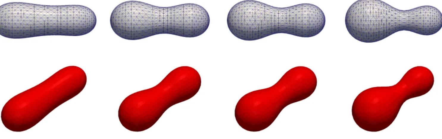
µ = α = 1, as well asβ = 0.46 and M0 = −33.5. As initial vesicle we take a varying-diameter cigar-like shape that hasvr= 0.75 anda(0) = 9.65. A simulation can be seen in Figure 4. As a comparison, we show the simula- tion withβ = 0 in Figure 5. Similarly to previous stud- ies, where an energy involving area difference elasticity terms was minimized, we also observe in our hydrody- namic model that less symmetric shapes occur when the ADE-energy contributions are taken into account.
B. Flow through a constriction
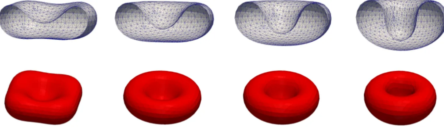
The numerical simulation of a vesicle flowing through a constriction can be seen in Figure 6. This example shows that membranes can drastically deform in order to pass through a constriction. This resembles the remarkable properties of red blood cells, which show a similar be- haviour when flowing through capillaries. Here we choose the initial shape of the interface to be a biconcave disco- cyte surface resembling a human red blood cell, with a reduced volume ofvr= 0.568 and a surface area ofa(0) = 2.24. As the computational domain we choose Ω = [−2,−1]×[−1,1]2∪[−1,1]×[−0.5,0.5]2∪[1,2]×[−1,1]2. We define∂2Ω ={2}×(−1,1)2and on∂1Ω we set no-slip conditions, except on the left hand part{−2} ×[−1,1]2, where we prescribe the inhomogeneous boundary condi- tions~g(~z) = ([1−z22−z23]+,0,0)T in order to model a Poiseuille-type flow. The remaining parameters are cho- sen as ˜µ= ˜µΓ = 1 andα= 0.1. In the larger domain Ω = [−3,−1]×[−1,1]2∪[−1,1]×[−0.5,0.5]2∪[1,4]×[−1,1]2, with the analogous boundary conditions, we also show the flow of four vesicles through a constriction, see Fig- ure 7.
C. Shearing for elliptical shapes
We conducted the following shearing experiments in Ω = [−2,2]3for an initial shape that is convex, with re- duced volume vr = 0.83 and a(0) = 6.95. The initial shape represents a local minimizer of the curvature en- ergyR
Γκ2 ds among all shapes with the same reduced volume and surface area. In order to model shear flow, we prescribe the inhomogeneous Dirichlet boundary con- dition~g(~z) = (z3,0,0)T on the top and bottom bound- aries∂1Ω = [−2,2]2× {±2}. The remaining parameters are given by ˜µ = 1, α = 0.05, and either ˜µΓ = 0.05
FIG. 1. Flow for a cup-like stomatocyte shape with vr = 0.65. The triangulations of Γh at times t = 0, 5, 10, 20. Here M0=−48.24 andβ= 0.053.
FIG. 2. Same as Figure 1 withβ= 0.
0.99998 1.00000 1.00002
0 5 10 15 20
v(t) / v(0) a(t) / a(0)
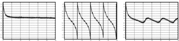
FIG. 3. The evolutions of the relative discrete volume v(t)/v(0), and the relative discrete surface areaa(t)/a(0) over time.
or ˜µΓ = 10. See Figures 8 and 9, where we observe tank treading (TT) for ˜µΓ = 0.05, and tumbling (TU) for ˜µΓ = 10. We stress that the tumbling occurs for a viscosity contrast of µ−/µ+ = 1, and so is only due to the chosen high surface viscosity ˜µΓ. The transition mo- tion TRc can be seen in Figure 10, where we have chosen
˜
µΓ = 1. A plot of the tilt angleθ for the simulations in Figures 8–10 can be seen in Figure 11.
In Table I we display the behaviour of the tilt angleθ for various values ofκ and ˜µΓ. Here the initial shapes of the vesicles, for a reduced volume of vr = 0.83 and surface area a(0) = 6.95, were chosen to be numerical approximations of local minimizers for the curvature en- ergyR
(κ−κ)2ds. These discrete local minimizers were obtained with the help of the gradient flow scheme from [19], and for the choices κ = ±5 they are displayed in Figure 12. The vesicle is then put in the same shear flow as in Figures 8–10. In fact, these three simulations cor- respond to the choiceκ= 0 in Table I. In the table we distinguish between tank treading (TT), the transition motions (TRc), (TRdc) and tumbling (TU), depending
FIG. 4. Flow for a varying-diameter cigar-like shape withvr= 0.75. The triangulations of Γhat timest= 0, 1, 10, 50. Here M0=−33.5 andβ= 0.46.
FIG. 5. Same as Figure 4 withβ= 0.
FIG. 6. Flow through a constriction. The plots show the interface Γhat timest= 0, 0.3, 0.5, 1, 1.4, 1.8.
FIG. 7. Flow through a constriction. The plots show the interface Γhat timest= 0, 0.4, 0.8, 1.2, 1.6, 2.2.4, 2.8.
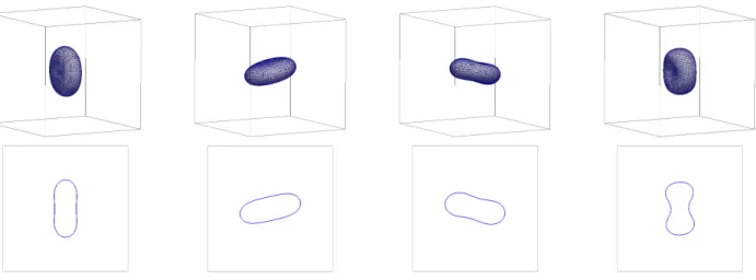
FIG. 8. Shear flow with ˜µ= 1 and ˜µΓ= 0.05 resulting in a tank treading (TT) motion. The plots show the interface Γhwithin Ω, as well as cuts through thex1-x3 plane, at timest= 0, 2.5, 5, 7.5.
on the behaviour of the tilt angleθ.
The results in Table I indicate that the values of the surface viscosity, at which the transitions between TT, TRc, TRdc and TU take place, strongly depend on the spontaneous curvature. For completeness, we visualize two tumbling motions forκ=±5 in Figures 13 and 14.
D. Shearing for biconcave discocyte shapes Here we use a scaled variant of the initial interface in Figure 6. In particular,vr = 0.568 and a(0) = 8.95.
For the remaining parameters we choose the values from §IV C. In particular, we let α = 0.05, and either
˜
µΓ = 0.05 or ˜µΓ = 10. The results can be seen in Figures 15 and 16. In both cases we observe a tumbling
FIG. 9. Shear flow with ˜µ= 1 and ˜µΓ= 10 resulting in a tumbling (TU) motion. The plots show the interface Γhwithin Ω, as well as cuts through thex1-x3 plane, at timest= 0, 2.5, 5, 7.5. The interface att= 10 is very close to the plot att= 2.5.
FIG. 10. Shear flow with ˜µ = 1 and ˜µΓ = 1 resulting in a motion in the transition regime with a continuous evolution of the inclination angle (TRc). The plots show the interface Γh within Ω, as well as cuts through the x1-x3 plane, at times t= 2.5, 5, 7.5, 10.
κ=−5
˜
µΓ θ
1 [0.05,0.17] TT 1.5 [0.02,0.17] TT 2 [0.01,0.14] TT 2.3 [-0.02,0.14] TRc 2.5 [-0.08,0.16] TRc 2.7 [-0.08,0.25] TRc
3 [−0.9,0.9] TRdc 4 [−0.9,1] TRdc
5 [−1.1,1.1] TRdc 10 [−1.3,1.4] TRdc 12.5 (−π2,π2] TU
15 (−π2,π2] TU 20 (−
π
2,π2] TU
κ= 0
˜
µΓ θ
0.1 [0.15,0.28] TT 0.2 [0.11,0.23] TT 0.4 [−0.04,0.08] TT 0.5 [−0.04,0.11] TRc
1 [−0.2,0.2] TRc 1.6 [−0.4,0.6] TRc
1.7 [−0.6,0.6] TRdc 3 [−1,1] TRdc
4 [−1.2,1.2] TRdc 8 [−1.4,1.5] TRdc 8.5 (−π2,π2] TU
9 (−π2,π2] TU 10 (−
π
2,π2] TU
κ= 5
˜
µΓ θ
0.1 [0.16,0.28] TT 0.2 [0.12,0.23] TT 0.4 [−0.02,0.13] TT 0.5 [−0.1,0.03] TRc
1 [−0.25,0.2] TRc 1.3 [−0.4,0.4] TRc
1.4 [−0.5,0.4] TRdc 2 [−0.8,0.7] TRdc
3 [−1.3,1.2] TRdc 3.3 [−1.4,1.4] TRdc 3.4 (−π2,π2] TU
4 (−π2,π2] TU 5 (−
π
2,π2] TU TABLE I. Eventual ranges ofθfor different values ofκand ˜µΓ.
-1.4 -1.2 -1 -0.8 -0.6 -0.4 -0.2 0 0.2 0.4 0.6 0.8 1 1.2 1.4
0 5 10 15 20 25 30
-1.4 -1.2 -1 -0.8 -0.6 -0.4 -0.2 0 0.2 0.4 0.6 0.8 1 1.2 1.4
0 5 10 15 20 25 30
-1.4 -1.2 -1 -0.8 -0.6 -0.4 -0.2 0 0.2 0.4 0.6 0.8 1 1.2 1.4
0 5 10 15 20 25 30
FIG. 11. The tilt angleθ for the computations in Figures 8–
10. They correspond to the motions TT, TU and TRc, re- spectively.
FIG. 12. The vesicles forκ=−5 (left) andκ= 5 (right) at timet= 0.
behaviour. In other situations, typically for small viscosity contrasts µ−/µ+ and for small membrane viscosities µΓ, a tank treading (TT) evolution occurs, see e.g. §IV C. This does not occur in our numerical simulations for this biconcave shape. We performed computations with the parameters (µ+, µ−,µ˜Γ, α) = (1,10−3,0,0.05), (1,10−3,0,10−3), (100,10−3,0,0.05), (10−2,10−2,0,0.05), (10−3,10−3,0.05,0.05), (10−2,10−2,0.05,0.05) without observing a tank treading (TT) motion.
E. Shearing for budded shape (two arms)
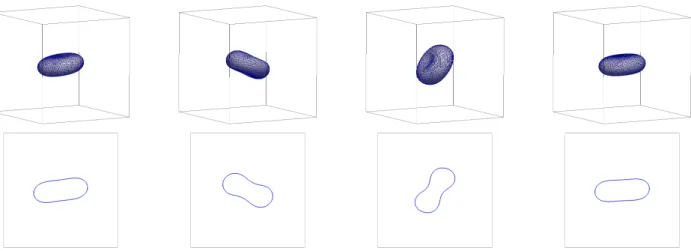
We start a scaled variant of the final shape from Fig- ure 4 in a shear flow experiment. In particular, the initial shape is axisymmetric, with reduced volume vr = 0.75 and a(0) = 5.43. We set ˜µ= ˜µΓ = 1, α= 0.05 and use the same domain and boundary conditions as in §IV C.
See Figure 17 for a run withβ = 0.1 and M0 =−33.5.
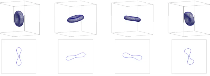
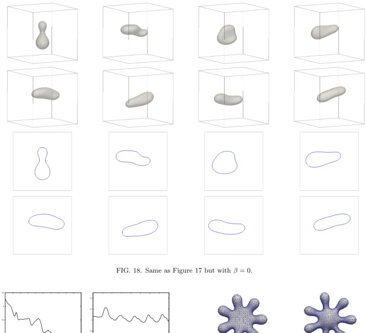
We observe that the shape of the vesicle changes dras- tically, with part of the surface growing inwards. This is similar to the shapes observed in Figure 1, where the presence of a lower reduced volume led to cup-like stoma- tocyte shapes. We repeat the same experiment forβ= 0 in Figure 18. Now the budding shape loses its strong non- convexity completely, as can be clearly seen in the plots of the two-dimensional cuts in Figure 18. Plots of the bending energy α E(Γh) are shown in Figure 19, where we recall that the energy inequality in (4) does not hold for the inhomogeneous boundary conditions employed in the present simulations.
F. Shearing for a seven-arm starfish
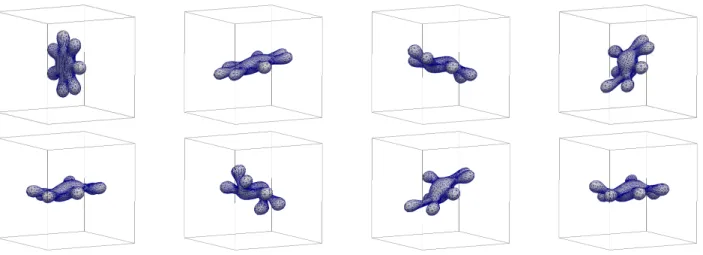
We consider simulations for a scaled version of the fi- nal shape from Barrettet al. [19, Fig. 23] with reduced volumevr = 0.38 and a(0) = 10.54 inside the domain Ω = [−2,2]3. We set ˜µ = ˜µΓ = α = 1. In order to maintain the seven-arm shape during the evolution we setβ = 0.05 and M0 = 180. The first experiment is for no-slip boundary conditions on∂Ω and shows that the seven arms grow slightly, see Figure 20. If we use the shear flow boundary conditions from§IV C, on the other hand, we observe the behaviour in Figure 21, where we have changed the value of α to 0.05. The vesicle can be seen tumbling, with the seven arms remaining intact.
Repeating the same experiment with β = 0 yields the simulation in Figure 22. Not surprisingly, some of the arms of the vesicle are disappearing.
G. Shearing for a torus
Here we use as the initial shape a Clifford torus with reduced volume vr = 0.71 and a(0) = 13.88. We let
˜
µ = ˜µΓ = 1, α = 0.05 and use the same domain and boundary conditions as in§IV C. See Figures 23, where the torus appears to tumble whilst undergoing strong de- formations.
V. CONCLUSIONS
We have introduced a parametric finite element method for the evolution of bilayer membranes by cou- pling a general curvature elasticity model for the mem- brane to (Navier–)Stokes systems in the two bulk phases and to a surface (Navier–)Stokes system. The model is based on work by Arroyo and DeSimone [43] and our main purpose was to study the influence of the area differ- ence elasticity (ADE) and of the spontaneous curvature on the evolution of the membrane. In contrast to most other works, we discretized the full bulk (Navier–)Stokes systems coupled to the surface (Navier–)Stokes system and for the first time coupled this to a bending energy involving ADE and spontaneous curvature.
The numerical simulations led to the following findings.
• The proposed numerical method conserves the vol- ume enclosed by the membrane and the surface area of the membrane to a high precision.
• For a flow through a constriction membranes de- formed drastically, which was resolved by the pro- posed parametric approach with no problems.
• The biconcave discocyte shape in our numerical simulations always led to a tumbling (TU) type be- haviour. In particular, also for very low viscosity contrasts and very low surface viscosities no tank treading (TT) motion was observed.
FIG. 13. Shear flow with ˜µ= 1 and ˜µΓ= 15 resulting in a tumbling (TU) motion. Hereκ=−5. The plots show the interface Γhwithin Ω, as well as cuts through thex1-x3plane, at timest= 10, 12.5, 15, 17.5. The interface att= 20 is very close to the plot att= 12.5.
FIG. 14. Shear flow with ˜µ= 1 and ˜µΓ= 5 resulting in a tumbling (TU) motion. Hereκ= 5. The plots show the interface Γh within Ω, as well as cuts through thex1-x3 plane, at timest= 10, 12.5, 15, 17.5. The interface att= 20 is very close to the plot att= 12.5.
FIG. 15. Shear flow with ˜µ= 1 and ˜µΓ= 0.05 resulting in a tumbling (TU) motion. The plots show the interface Γhwithin Ω, as well as cuts through thex1-x3 plane, at timest= 0, 2.5, 5, 7.5. The interface att= 10 is very close to the plot att= 2.5.
FIG. 16. Shear flow with ˜µ= 1 and ˜µΓ= 10 resulting in a tumbling (TU) motion. The plots show the interface Γhwithin Ω, as well as cuts through thex1-x3 plane, at timest= 0, 2.5, 5, 7.5. The interface att= 10 is very close to the plot att= 2.5.
FIG. 17. Shear flow for a budding shape with ˜µ= ˜µΓ= 1. Hereβ= 0.1 and M0 =−33.5. The plots show the interface Γh within Ω, as well as cuts through thex1-x3 plane, at timest= 0, 5, 15, 17.5, 20, 25, 27.5, 32.5.
• The transition from a tank treading (TT) motion to a transition motion (TR) and to a tumbling (TU) motion depended strongly on the surface viscosity.
We observed that the surface viscosity alone with no viscosity contrast between inner and outer fluid can lead to a transition from tank treading to a
TR-motion and to tumbling.
• The surface viscosity at which a transition be- tween the different motions TT, TR and TU oc- cur, strongly depends on the spontaneous curva- ture. In particular, we observed that for negative
FIG. 18. Same as Figure 17 but withβ= 0.
7.5 8 8.5 9 9.5
0 5 10 15 20 25 30 35 40 45 50
1.6 1.8 2 2.2 2.4
0 5 10 15 20 25 30 35 40
FIG. 19. The bending energyα E(Γh) for the computations in Figures 17 and 18.
spontaneous curvature all transitions occurred for larger values of the surface viscosity. For positive spontaneous curvature we observed that tumbling occurred already for much smaller values of the sur- face viscosity. Here we recall that our sign conven- tion for curvature means that spheres have negative mean curvature.
• In some cases, shear flow can lead to drastic shape changes, in particular for the ADE-model. For ex- ample, we observed the transition of a budded pear- like shape to a cup-like stomatocyte shape in shear flow if an ADE-model was used for the curvature elasticity.
FIG. 20. Flow for a seven-arm figure with vr = 0.38. Here β= 0.05 andM0= 180. The triangulations Γhat timest= 0 and 5.
• The ADE-model can also lead to starfish-type shapes with several arms, see e.g. [1, 15]. In com- putations for a seven-arm starfish for a model in- volving an ADE type energy, we observed that in shear flow the overall structure seems to be quite robust. In particular, the seven arms deformed but remained present even in a tumbling motion. How- ever, arms tend to disappear if the area difference elasticity term is neglected.
Thus we have shown that the proposed numerical method is a robust tool to simulate bilayer membranes for quite general models which in particular take the full hydrody-
FIG. 21. Shear flow for a budding shape with ˜µ= ˜µΓ = 1. Hereβ= 0.05 andM0 = 180. The plots show the interface Γh within Ω at timest= 0, 2.5, 5, 7.5, 10, 12.5, 15, 17.5.
FIG. 22. Same as Figure 21 withβ= 0.
FIG. 23. Shear flow for a torus with ˜µ= ˜µΓ= 1. The plots show the interface Γhwithin Ω, as well as cuts through thex1-x3 plane, at timest= 0, 2.5, 5, 7.5. The interface att= 10 is very close to the plot att= 2.5.
namics and a curvature model involving area difference elasticity and spontaneous curvature into account.
Acknowledgement. The authors gratefully acknowl- edge the support of the Deutsche Forschungsgemein- schaft via the SPP 1506 entitled “Transport processes at fluidic interfaces” and of the Regensburger Univer- sit¨atsstiftung Hans Vielberth.
[1] U. Seifert, Adv. Phys.46, 13 (1997).
[2] T. Baumgart, S. T. Hess, and W. W. Webb, Nature425, 821 (2003).
[3] H. Noguchi and G. Gompper, PNAS102, 14159 (2005).
[4] J. L. McWhirter, H. Noguchi, and G. Gompper, Proc.
Natl. Acad. Sci. USA106, 6039 (2009).
[5] P. Canham, J. Theor. Biol.26, 61 (1970).
[6] W. Helfrich, Z. Naturforsch.28c, 693 (1973).
[7] S. Martens and H. T. McMahon, Nat. Rev. Mol. Cell.
Biol.9, 543 (2008).
[8] M. M. Kamal, D. Mills, M. Grzybek, and J. Howard, PNAS106, 22245 (2009).
[9] S. Svetina, A. Ottova-Leitmannov´a, and R. Glaser, J.
Theor. Biol.94, 13 (1982).
[10] S. Svetina and B. Zeks, Biomed. Biochim. Acta42, 86 (1983).
[11] S. Svetina and B. Zeks, Biochem. Biophys. Acta42, 84 (1989).
[12] L. Miao, U. Seifert, M. Wortis, and H.-G. D¨obereiner, Phys. Rev. E49, 5389 (1994).
[13] P. Ziherl and S. Svetina, Europhys. Lett.70, 690 (2005).
[14] U. Seifert, K. Berndl, and R. Lipowsky, Phys. Rev. A 44, 1182 (1991).
[15] W. Wintz, H.-G. D¨obereiner, and U. Seifert, Europhys.
Lett.33, 403 (1996).
[16] U. F. Mayer and G. Simonett, Interfaces Free Bound.4, 89 (2002).
[17] U. Clarenz, U. Diewald, G. Dziuk, M. Rumpf, and R. Rusu, Comput. Aided Geom. Design21, 427 (2004).
[18] G. Dziuk, Numer. Math.111, 55 (2008).
[19] J. W. Barrett, H. Garcke, and R. N¨urnberg, SIAM J.
Sci. Comput.31, 225 (2008).
[20] Q. Du, C. Liu, R. Ryham, and X. Wang, Nonlinearity 18, 1249 (2005).
[21] M. Franken, M. Rumpf, and B. Wirth, Int. J. Numer.
Anal. Model.10, 116 (2013).
[22] A. Bonito, R. H. Nochetto, and M. S. Pauletti, J. Com- put. Phys.229, 3171 (2010).
[23] Q. Du, C. Liu, and X. Wang, J. Comput. Phys.198, 450 (2004).
[24] C. M. Elliott and B. Stinner, J. Comput. Phys.229, 6585 (2010).
[25] S. Bartels, G. Dolzmann, R. H. Nochetto, and A. Raisch, Interfaces Free Bound.14, 231 (2012).
[26] M. Mercker, A. Marciniak-Czochra, T. Richter, and D. Hartmann, SIAM J. Appl. Math.73, 1768 (2013).
[27] Q. Du, C. Liu, R. Ryham, and X. Wang, Phys. D238, 923 (2009).
[28] G. Boedec, M. Leonetti, and M. Jaeger, J. Comput.
Phys.230, 1020 (2011).
[29] M. Rahimi and M. Arroyo, Phys. Rev. E 86, 011932 (2012).
[30] D. S. Rodrigues, R. F. Ausas, F. Mut, and G. C.
Buscaglia, “A semi-implicit finite element method for vis-
cous lipid membranes,” (2014),http://arxiv.org/abs/
1409.3581.
[31] D. Salac and M. Miksis, J. Comput. Phys. 230, 8192 (2011).
[32] D. Salac and M. J. Miksis, J. Fluid Mech. 711, 122 (2012).
[33] A. Laadhari, P. Saramito, and C. Misbah, J. Comput.
Phys.263, 328 (2014).
[34] V. Doyeux, Y. Guyot, V. Chabannes, C. Prud’homme, and M. Ismail, J. Comput. Appl. Math.246, 251 (2013).
[35] T. Biben, K. Kassner, and C. Misbah, Phys. Rev. E72, 041921 (2005).
[36] D. Jamet and C. Misbah, Phys. Rev. E76, 051907 (2007).
[37] S. Aland, S. Egerer, J. Lowengrub, and A. Voigt, J.
Comput. Phys.277, 32 (2014).
[38] Y. Kim and M.-C. Lai, J. Comput. Phys. 229, 4840 (2010).
[39] Y. Kim and M.-C. Lai, Phys. Rev. E86, 066321 (2012).
[40] W.-F. Hu, Y. Kim, and M.-C. Lai, J. Comput. Phys.
257, 670 (2014).
[41] W. R. Dodson and P. Dimitrakopoulos, Phys. Rev. E84, 011913 (2011).
[42] A. Farutin, T. Biben, and C. Misbah, J. Comput. Phys.
275, 539 (2014).
[43] M. Arroyo and A. DeSimone, Phys. Rev. E79, 031915, 17 (2009).
[44] M. Arroyo, A. DeSimone, and L. Heltai, “The role of membrane viscosity in the dynamics of fluid membranes,”
(2010),http://arxiv.org/abs/1007.4934.
[45] J. W. Barrett, H. Garcke, and R. N¨urnberg, “A stable numerical method for the dynamics of fluidic biomem- branes,” (2014), preprint No. 18/2014, University Re- gensburg, Germany.
[46] J. W. Barrett, H. Garcke, and R. N¨urnberg, “Finite element approximation for the dynamics of asymmetric fluidic biomembranes,” (2015), preprint No. 03/2015, University Regensburg, Germany.
[47] U. Seifert, L. Miao, H.-G. D¨obereiner, and M. Wortis, inThe Structure and Conformation of Amphiphilic Mem- branes, Springer Proceedings in Physics, Vol. 66, edited by R. Lipowsky, D. Richter, and K. Kremer (Springer- Verlag, Berlin, 1992) pp. 93–96.
[48] W. Wiese, W. Harbich, and W. Helfrich, J. Phys. Con- dens. Matter4, 1647 (1992).
[49] B. Bozic, S. Svetina, B. Zeks, and R. Waugh, Biophys.
J.61, 963 (1992).
[50] L. E. Scriven, Chem. Eng. Sci.12, 98 (1960).
[51] T. J. Willmore, An. S¸ti. Univ. “Al. I. Cuza” Ia¸si Sect¸. I a Mat. (N. S.)11B, 493 (1965).
[52] M. Faivre,Drops, vesicles and red blood cells: Deforma- bility and behavior under flow, Ph.D. thesis, Universit´e Joseph Fourier, Grenoble, France (2006).
[53] D. Abreu, M. Levant, V. Steinberg, and U. Seifert, Adv.
Colloid Interface Sci.208, 129 (2014).
[54] E. B¨ansch, Numer. Math.88, 203 (2001).
[55] R. Capovilla and J. Guven, J. Phys. Condens. Matter16, 2187 (2004).
[56] D. Lengeler, “On a Stokes-type system arising in fluid vesicle dynamics,” (2015), (in preparation).
[57] J. W. Barrett, H. Garcke, and R. N¨urnberg, J. Sci.
Comp.63, 78 (2015).
[58] V. Kantsler and V. Steinberg, Phys. Rev. Lett. 96, 036001 (2006).
[59] N. J. Zabusky, E. Segre, J. Deschamps, V. Kantsler, and
V. Steinberg, Phys. Fluids23, 041905 (2011).
[60] C. Misbah, Phys. Rev. Lett.96, 028104 (2006).
[61] H. Noguchi and G. Gompper, Phys. Rev. Lett.98, 128103 (2007).
[62] A. Yazdani and P. Bagchi, Phys. Rev. E 85, 056308 (2012).
[63] A. Farutin and C. Misbah, Phys. Rev. Lett.109, 248106 (2012).