Playing with Boolean Blocks, Part I:
Post’s Lattice with Applications to Complexity Theory
1Elmar B¨ ohler
2, Nadia Creignou
3, Steffen Reith
4, and Heribert Vollmer
5Introduction
Let us imagine children playing with a box containing a large number of building blocks such as LEGOTM, fischertechnik, Polydron, or something similar. Each block belongs to a certain class (given by, e. g., color, shape, or size) and usually the number of different such classes is relatively small. It is amazing to see how involved the constructions are that can be built by the kids. From an abstract point of view, one might ask if there is something similar to all objects that may be built using only blocks from some given classes, or if a given object (i.e., given by some description) can be constructed using the available blocks. These questions become interesting from a theoretical point of view if the number of different types or classes of blocks is finite, but from each type of block we have an infinite number of “copies” available for construction.
In this (and the upcoming January) complexity theory column we will play with Boolean blocks.
In the present issue we will mainly consider Boolean functions as basic blocks. We want to use them as gates in the construction of Boolean circuits. Thus, the way of building blocks together here is the operation of soldering. In the next issue we will use Boolean constraints, i. e., Boolean relations, to construct so called conjunctive queries to a database.
To be a bit more formal, let B be a set of Boolean functions. By [B] we denote the class of all Boolean functions that can be obtained from functions out ofB∪ {id}by soldering them together, i. e., [B] consists of all arbitrary compositions of functions fromB∪{id}. Here,id denotes the unary identity, id(x) = x. We will see that for certain “syntactical” reasons we always have to include the identity. Thus, [B] consists of all functions ofB∪ {id}plus those, that can be obtained by the following rule: Iff(x1, . . . , xn)∈[B] andX1, . . . , Xn are either Boolean variables or elements from [B], then f(X1, . . . , Xn) ∈[B], too. Note that we are able to permute and identify variables of a Boolean function by this operation. We say that a classB of Boolean functions isclosed if [B] =B which means that we cannot generate new Boolean functions by composing functions out ofB.
It is interesting to note that [B] is exactly the class of Boolean functions that can be computed by circuits with gates from B, or, equivalently, can be defined by propositional formulas with connectives fromB. We will come back to this observation in Sect. 1.2.
In the forties of the previous century, Emil Post obtained a complete list of all closed classes of Boolean functions, nowadays calledPost’s lattice, and moreover, he proved that each of them has a finite basis and obtained a list of bases for all closed classes [Pos41] (see Figs. 1 and 2). Closed classes are also referred to as clones, a term used in universal algebra. We will see in the second part of this column that the substantial clone theory can help us to obtain elegant and short proofs
1Elmar B¨c ohler, Nadia Creignou, Steffen Reith and Heribert Vollmer, 2003. Supported in part by ´EGIDE 05835SH, DAAD D/0205776 and DFG VO 630/5-1.
2Theoretische Informatik, Fachbereich Mathematik und Informatik, Universit¨at W¨urzburg, Am Hubland, 97072 W¨urzburg, GERMANY,boehler@informatik.uni-wuerzburg.de.
3Laboratoire d’informatique fondamentale, Facult´e des sciences de Luminy, Universit´e de la M´editerran´ee, 163 avenue de Luminy, 13288 Marseille cedex 9, FRANCE,creignou@lidil.univ-mrs.fr
4Lengfelderstr. 35b, 97078 W¨urzburg, GERMANY,streit@streit.cc.
5Theoretische Informatik, Fachbereich Informatik, Universit¨at Hannover, Appelstraße 4, 30167 Hannover, GER- MANY,vollmer@thi.uni-hannover.de.
for results concerning constraint satisfaction problems. In the present part I we will use Post’s lattice as a tool in complexity examinations of Boolean circuits and propositional formulas.
A description of Post’s lattice (without a proof of the classification, but a proof of the finite basis theorem) can be found in [Pip97, Chap. 1]. A complete and self-contained presentation of Post’s result is given in [JGK70]. Different and much shorter proofs can be found in [Ugo88, Zve00].
As just mentioned, Post’s lattice can be a very helpful tool for complexity studies of Boolean circuits and propositional formulas. Before turning to a detailed discussion of the lattice in Sect. 1 we want to show the reader a glimpse of what is ahead in Sect. 2 where we turn to applications in complexity theory. The famous Cook-Levin-Theorem states that the problem, given a propositional formula or circuit to determine if it is satisfiable, is NP-complete [Coo71, Lev73]. A question that arises immediately is if there are subclasses of propositional formulas for which the satisfiability problem is easier, e. g., efficiently solvable. One direction one might pursue is to restrict the types of Boolean connectives allowed. Instead of the usual formulas or circuits over{∧,∨,¬}one might for example restrict oneself to {∧,⊕}. Since [B] is the class of those functions that can be defined using propositional formulas with allowed Boolean connectives taken fromB, this question is most naturally studied in connection to Post’s lattice: Allowing connectives from B is the same as allowing connectives from [B]. Lewis in 1979 [Lew79] obtained the remarkable result that the satisfiability of propositional formulas is NP-complete if and only if the connective x∧ ¬y can be represented (in Post’s lattice, this corresponds to the class S1). We will give a very short proof of Lewis’ result in Sect. 2. Coming back to the above example set {∧,⊕}, satisfiability turns out to be again NP-complete, since, as we will see, [{∧,⊕}] is the class R0 in Post’s lattice, a superclass of S1.
1 Closed Classes of Boolean Functions: Post’s Lattice
Boolean circuits and Boolean functions attract and deserve a lot of attention in computer science, and the theory behind them is exhaustively used in circuit design and various other important fields. We will have a look at superposition, i. e., the mathematical operations that correspond to operations carried out when soldering Boolean circuits. Whether or not a Boolean function can be described by a Boolean circuit depends solely on the sort of gates one is allowed to use in the construction of the circuit. There are classes of Boolean functions that are closed under superposition: In this section we will discuss these and the result from E. L. Post [Pos41] who identified and characterized each of them.
1.1 Boolean Functions
An n-ary Boolean function is a function from {0,1}n to{0,1}. There are several ways to describe an n-ary Boolean function f. One is to explicitly specify for each n-tuple a1, . . . , an the function value f(a1, . . . , an), i. e., to construct a lookup table for all possible inputs of the function, the so calledtruth-table. This form of representation is often very inconvenient, since the truth table has exponentially many (exactly 2n) entries.
Since we have binary function values, every Boolean function also defines an n-ary relation:
The set of all n-tuples α with f(α) = 1. A second possibility to describe a Boolean function thus is by listing all of these, but again, we will have up to exponentially many tuples.
Much more compact methods to describe Boolean functions are Boolean circuits and proposi- tional formulas, which we will define formally in the next subsection.
Throughout the text, we will refer to some basic Boolean functions (that are often used as gates when building circuits or as connectives when building formulas), with the notations listed below:
– 0-ary Boolean functions: c0 =def 0 andc1 =def 1.
(We write 0 and 1 in formulas.)
– 1-ary Boolean functions: id(x) =defx; and not(x) = 1 iffx= 0.
(In formulas we simply write xforid(x) and x or¬xfornot(x).)
– some prominent 2-ary Boolean functions: and(x, y) = 1 iff x = y = 1, or(x, y) = 0 iff x=y = 0, xor(x, y) = 1 iff x 6=y,eq(x, y) = 1 iff x=y,imp(x, y) = 0 iff x = 1 and y= 0, and nand(x, y) = 0 iff x=y= 1.
(In formulas, we use∧,∨,⊕,↔,→,|, resp., all operators are used in infix notation.) 1.2 Assembling Boolean Functions – B-Circuits and Superposition
LetB be a set of Boolean functions. An n-input B-circuit (or, an n-input circuit overbasis B) is a directed, acyclic graph where each node is labeled either with a variable xi,i= 1,2,3, . . . , n, or a function from B. We will call the nodes of this graph gates. The number of edges (also called wires) pointing into a gate is called fan-in, the number of wires leaving a gate is called fan-out of that gate. For reasons that will become clear shortly, we also order the edges pointing into a gate. If a wire leaving gateu is pointing into gate v, we say that u is apredecessor gate ofv. The gates labeled with a variable must have a fan-in of 0; we call theseinput gates. The fan-in of gates labeled with a Boolean function has to be as large as the arity of that function. We mark one particular gate and call itoutput gate. Note that an input-gate can be the output-gate, too. Hence the functionid can be computed byB-circuits for any B.
The computation of an n-inputB-circuitC proceeds as we describe next. Given ann-bit input stringx=a1a2. . . an, every gate inC computes a Boolean value as follows: A gate vlabeled with a variablexi returns the bitai. A gatev of fan-inklabeled by a Boolean functionf computes the valuef(b1, . . . , bk), whereb1, . . . , bkare the values computed by the predecessor gates ofv, ordered according to the order of those wires connecting v with its predecessors. The value of C on input x is the value computed by the output gate. In this way, C computes an n-ary Boolean function, which we denote byfC. (We will use the notationsfC(a1. . . an) andfC(a1, . . . , an) interchangeably with identical meaning.) The class CIRC(B) is the set of all functions that can be computed by B-circuits.
Note that a propositional formula can be seen as a circuit where the fan-out of each node is at most 1. So we treat B-formulas as a special case of (tree-like) B-circuits.
Given a fixed set B, what are the Boolean functions that can be computed by a B-circuit?
More precisely, we are looking for a set of operations such that CIRC(B) can be obtained as the closure ofB under these. The operations have to describe in a mathematical way what “soldering some given circuits together” means.
First note that surely every f from B is in CIRC(B): Just build a circuit that has as many input nodes as f has arguments, and draw an edge from every input node to one additional node, labeled with f. Suppose we have a B-circuit C1 computing the n-ary Boolean function fC1, and anotherB-circuit C2 computing m-aryfC2. Now we can derive newB-circuits by performing one of the following operations:
(i) We get a new circuit C10 by just adding one input node to C1. Since we do not add any new edges, the new node has no influence on the computed Boolean function besides the higher
arity. We call this operation introduction of a fictive variable and get for all a1, . . . , an+1 ∈ {0,1}: fC0
1(a1, . . . , an+1) = fC1(a1, . . . , an). In general, we will say a variable of a Boolean function (an input gate of a circuit) is fictive, if the value of the function (the circuit) never depends on this variable (this input gate).
(ii) We may obtain circuitC10 fromC1by arbitrarily permuting the input variables. This operation will be called permutation of variables and if π ∈ Sn is our permutation, we get for all a1, . . . , an∈ {0,1}: fC0
1(a1, . . . , an) =fC1(aπ−1(1), . . . , aπ−1(n)).
(iii) Since the fan-out of gates is not restricted whatsoever, we can remove all outgoing edges of one input gate xi of C1 and assign them to another input gate xj. After this operation, xi
is a fictive gate and we drop it. The thus derived circuit C10 is a B-circuit and computes a function of arityn−1, given byfC0
1(a1, . . . , ai−1, ai+1, . . . , an) =fC1(a1, . . . , ai−1, aj, ai+1, . . . , an). We call this operationidentification of variables.
(iv) If we replace input gatexnof C1 by the whole circuitC2, i. e., we replacexn with the output gate ofC2 and we replace inC2 every input gatexj (for 1≤j≤m) byxn−1+j, we get a new B-circuitC0 of arity n+m−1. For the Boolean function fC0 obtained in this way, we have:
fC0(a1, . . . , an−1, an, . . . , an+m−1) =fC1(a1, . . . , an−1, fC2(an, . . . , an+m−1)). This operation is calledsubstitution.
The important observation now is that every B-circuit can be obtained by a sequence of these operations. Or, speaking about Boolean functions instead of circuits: The operations (i)–(iv) though defined on circuits correspond immediately to operations on Boolean functions. Define the closure of a set B of Boolean functions under superposition, denoted by [B], to be the set of those functions that can be obtained from functions in B ∪ {id} by a finite sequence of applications of (i)–(iv). It is interesting to note that superposition is equivalent to arbitrary composition of Boolean functions and introduction of fictive variables. So f ∈ [B] if and only if f ∈ B ∪ {id} or there is a g ∈ [B] and X1, . . . , Xn, that are either variables or functions from [B], such that f =g(X1, . . . , Xn).
Superposition on the level of Boolean functions corresponds to soldering on the level of circuits, thus [B] = CIRC(B). We conclude that, if we want to know which Boolean functions can be computed by B-circuits, we do not have to talk about circuits at all: It suffices to study the closures of classes of Boolean functions under superposition.
Example 1.1. Letf(x, y) =def x∧y be a Boolean function. Is the function and(x, y) in [f]? (We use [f] as a shorthand for [{f}].) To answer this question, we have to find a composition of f’s that is equal toand(x, y). In this case it is easy to verify thatand(x, y) =f(x, f(x, y)).
1.3 Post’s Lattice
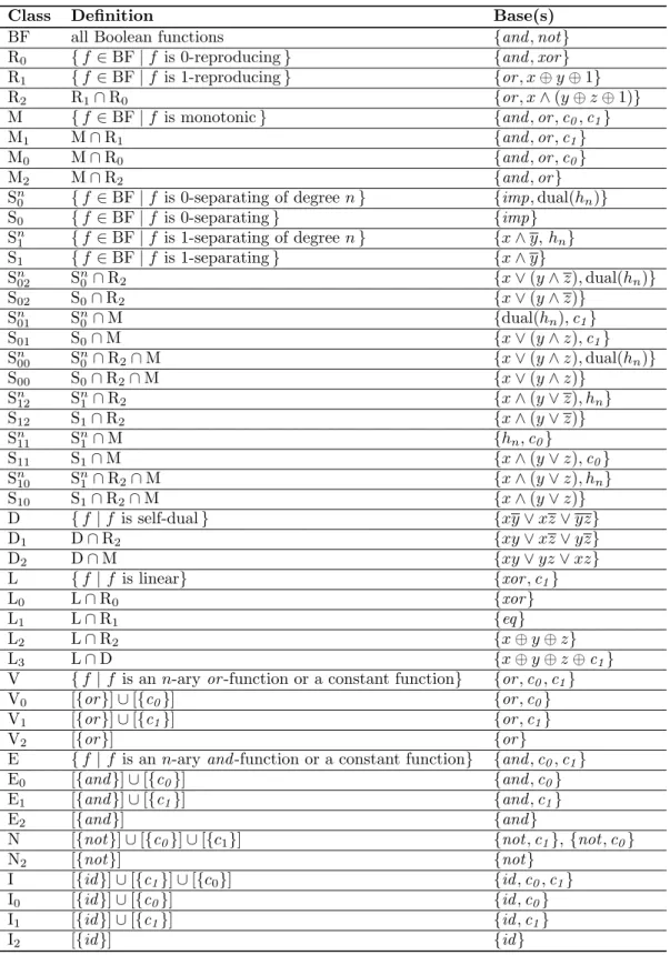
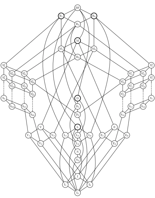
We say a set of Boolean functions B is a clone (or, B is closed) if B = [B], i. e., no new functions can be derived from compositions of functions from B∪ {id}. Every set B0 ⊆ B with [B0] = B is called a base (or basis) of B. We also say that such a set B0 is complete in B. As mentioned before, all closed classes of Boolean functions were identified by Post [Pos41], who also found a finite basis for each of them (see Fig. 1). Post also detected the very useful inclusion structure of the classes (see Fig. 2), hence the namePost’s graph or (as we will shortly prove that the structure is a lattice)Post’s lattice.
We would like to mention that the names of the classes in Fig. 2 are not those Post used originally. Post was not only interested in closed classes of Boolean functions, but he additionally considered so called “iterative classes” which are missing some of the closure properties of our notion of superposition. This leads to the idiosyncrasy that if we used Post’s names, we would have, e. g., classes P1,P3,P5,P6, but no P2 and P4. The terminology used in Fig. 2 was developed by Klaus Wagner in an attempt to construct a consistent scheme of names for closed classes, and further propagated in [RW00, RV00].
We want to introduce some clones:
– BF is the class of all Boolean functions.
– For a∈ {0,1}, a Boolean function f is called a-reproducing if f(a, . . . , a) =a. The clones Ra contain alla-reproducing Boolean functions.
– For (a1, . . . , an),(b1, . . . , bn)∈ {0,1}n, we say (a1, . . . , an)≤(b1, . . . , bn) ifai≤bi for 1≤i≤ n. An n-ary Boolean functionf is calledmonotonic if for all α, β ∈ {0,1}n holds: If α ≤β then f(α) ≤ f(β). Typical monotonic Boolean functions are and and or. The class of all monotonic Boolean functions is denoted by M.
– A Boolean functionf is calledself-dual if for all a1, . . . , an∈ {0,1}we have f(a1, . . . , an) =
¬f(a1, . . . , an). Therefore constants are never self-dual and simple self-dual functions are id and not. The class of all self-dual Boolean functions is called D.
– Boolean functions that can be defined with a linear formula are called linear, i. e., an n- ary function f is linear if there exist constants c0, . . . , cn ∈ {0,1} such that f(x1, . . . , xn) = c0⊕c1x1⊕ · · · ⊕cnxn. (Here and in the following, we do not distinguish between a Boolean function and the defining propositional formula. Also, for variables x, y we use xy as a shorthand for x∧y.) The typical linear functions are xor and eq. The class of all linear Boolean functions is called L.
– Let T ⊆ {0,1}n and a ∈ {0,1}. We call T a-separating if there exists an i ∈ {1, . . . , n}
such that for all (b1, . . . , bn)∈T holds bi =a. A Boolean functionf is called a-separating if f−1(a) is a-separating. The function f is called a-separating of level k if every T ⊆ f−1(a) with |T|=k is a-separating. The classes of alla-separating functions are called Sa and the classes of a-separating functions of levelk are called Ska.
– The class E is the class of all Boolean functions that can be described by formulas build over ∧, 0 and 1: E = {f | n ∈ N and f(x1, . . . , xn) = c0 ∧(c1∨x1)∧. . .∧(cn∨xn) for some constants ci, 0 ≤ i ≤ n}. Analogously, V is the class of Boolean functions that can be described by formulas build over∨, 0 and 1. (“E” and “V” stand for “et” and “vel”, the Latin names of AND and OR.)
– The class I2 contains all projections (i.e., all Boolean functions Ikn with Ikn(a1, . . . , an) = ak for alla1, . . . , an∈ {0,1}), and I contains all projections and additionally all constants (i.e., all Boolean functions cna, a∈ {0,1}, withcna(a1, . . . , an) = a for all a1, . . . , an ∈ {0,1}). N2 contains all projections and all negations of projections. The class N contains N2 and all constants.
All other classes in Post’s graph can be obtained from the above by intersection, as we illustrate next. Let Aand B be clones and
Class Definition Base(s)
BF all Boolean functions {and,not}
R0 {f ∈BF|f is 0-reproducing} {and,xor}
R1 {f ∈BF|f is 1-reproducing} {or, x⊕y⊕1}
R2 R1∩R0 {or, x∧(y⊕z⊕1)}
M {f ∈BF|f is monotonic} {and,or,c0,c1}
M1 M∩R1 {and,or,c1}
M0 M∩R0 {and,or,c0}
M2 M∩R2 {and,or}
Sn0 {f ∈BF|f is 0-separating of degree n} {imp,dual(hn)}
S0 {f ∈BF|f is 0-separating} {imp}
Sn1 {f ∈BF|f is 1-separating of degree n} {x∧y,hn}
S1 {f ∈BF|f is 1-separating} {x∧y}
Sn02 Sn0∩R2 {x∨(y∧z),dual(hn)}
S02 S0∩R2 {x∨(y∧z)}
Sn01 Sn0∩M {dual(hn),c1}
S01 S0∩M {x∨(y∧z),c1}
Sn00 Sn0∩R2∩M {x∨(y∧z),dual(hn)}
S00 S0∩R2∩M {x∨(y∧z)}
Sn12 Sn1∩R2 {x∧(y∨z), hn}
S12 S1∩R2 {x∧(y∨z)}
Sn11 Sn1∩M {hn,c0}
S11 S1∩M {x∧(y∨z),c0}
Sn10 Sn1∩R2∩M {x∧(y∨z), hn}
S10 S1∩R2∩M {x∧(y∨z)}
D {f |f is self-dual} {xy∨xz∨yz}
D1 D∩R2 {xy∨xz∨yz}
D2 D∩M {xy∨yz∨xz}
L {f |f is linear} {xor,c1}
L0 L∩R0 {xor}
L1 L∩R1 {eq}
L2 L∩R2 {x⊕y⊕z}
L3 L∩D {x⊕y⊕z⊕c1}
V {f |f is ann-ary or-function or a constant function} {or,c0,c1}
V0 [{or}]∪[{c0}] {or,c0}
V1 [{or}]∪[{c1}] {or,c1}
V2 [{or}] {or}
E {f |f is ann-ary and-function or a constant function} {and,c0,c1}
E0 [{and}]∪[{c0}] {and,c0}
E1 [{and}]∪[{c1}] {and,c1}
E2 [{and}] {and}
N [{not}]∪[{c0}]∪[{c1}] {not,c1},{not,c0}
N2 [{not}] {not}
I [{id}]∪[{c1}]∪[{c0}] {id,c0,c1}
I0 [{id}]∪[{c0}] {id,c0}
I1 [{id}]∪[{c1}] {id,c1}
I2 [{id}] {id}
Figure 1: List of all Boolean clones with bases (hn = Wn+1
i=1 x1· · ·xi−1xi+1· · ·xn+1 and dual(f)(a1, . . . , an) =¬f(a1, . . . , an)).
R1 R0
BF
R2
M
M1 M0
M2
S20
S30
S0
S202
S302
S02
S201
S301
S01
S200
S300
S00
S21
S31
S1
S212
S312
S12
S211
S311
S11
S210
S310
S10
D D1
D2
L
L1 L0
L2
L3
V
V1 V0
V2
E E0
E1
E2
I
I1 I0
I2
N2
N
Figure 2: Graph of all Boolean clones
– letAuB be the largest clone that is contained in both Aand B, and – letAtB be the smallest clone that contains bothA and B.
Note thatA∩B ⊆[A∩B]. On the other hand we haveA∩B ⊆Aand hence [A∩B]⊆[A] =A.
Analogously we obtain [A∩B] ⊆ [B] = B, which gives us [A∩B] ⊆ A∩B. We conclude that [A∩B] =A∩B, henceA∩B is again a clone. But sinceAuB is the largest clone that is contained in bothA and B we have thatA∩B ⊆AuB. Since by definition, AuB ⊆A∩B, we conclude A∩B =AuB. Similarly we can show that [A∪B] = AtB holds. It is easy to check, that u and tare both associative and commutative. Besides that,Au(AtB) =A andAt(AuB) =A hold, so the Boolean clones form a lattice.
Example 1.2. The class E1 consists of functions from E that are also 1-reproducing, E1= E∩R1. Similarly, E0 = E∩R0. The class E2 finally consists of all functions from E that are both 1- reproducing and 0-reproducing. As a general mnemonic, functions from classes with index 0 are 0-reproducing, functions from classes with index 1 are 1-reproducing, and functions from classes with index 2 are both. This implies that, while E contains all constant functions, the only constant functions in E0 are constant 0 functions, the only constant functions in E2 are constant 1 functions, and that E2 does not contain any constant functions. This is similarly valid for other classes as Ri, Mi, Li, Vi, Ei, Ni and Ii, where iis empty or an index 0, 1 or 2. Observe that D is excluded here since constant functions are never self-dual.
The well known Post’s classes are those classes B in Post’s lattice with the properties that B ( BF and that for every B0 with B ( B0 ⊆ BF we obtain [B0] = BF, hence they are the maximal classes which do not contain all Boolean functions; in other words: Post’s classes are the dual atoms of Post’s lattice. (Sometimes they are simply called maximal clones [Sze86].) There are five such classes, namely R0, R1, M, D, and L; these are circled bold in Fig. 2. This suggests a very convenient test whether a given function f (or setB) is complete in the sense that [f] = BF ([B] = BF): One just has to make sure that f (or B) is not contained in one of Post’s classes.
Example 1.3. Consider the Boolean functionnand. Clearlynand 6∈R0 andnand 6∈R1. Moreover we havenand 6∈M, because (0,0)≤(1,1), but nand(0,0)6≤nand(1,1). Thenand-function is not self-dual sincenand(0,1)6=¬nand(1,0). Finally note thatnand is not linear. To show this suppose that nand is linear. In this case we have nand(x, y) =c0⊕c1x⊕c2y. Becausenand(0,0) = 1 we have c0 = 1, bynand(1,0) = 1 we obtain c1 = 0 and by nand(0,1) = 1 we obtainc2 = 0 too. But this is a contradiction since nand is not a constant function. Since nand is not contained in one of the five maximal clones we conclude that [nand] = BF. Hence each Boolean function can be implemented by anand-circuit.
Another interesting and useful aspect isduality. We say a functionf is the dual function ofgif they both have the same aritynand for all a1, . . . , an∈ {0,1}holds f(a1, . . . , an) =g(a1, . . . , an).
We define dual(f) to be the dual function off and for a set of Boolean functionsB we let dual(B) = {dual(f)|f ∈B}.
Duality Principle. Letα∈ {0,1}n, letgbe anm-ary andf1, . . . , fmben-ary Boolean functions, and leth(α) =def g(f1(α), . . . , fm(α)). Then dual(h)(α) = dual(g)(dual(f1)(α), . . . ,dual(fm)(α)).
This implies that, if a Boolean function f is computed by some B-circuit C, then dual(f) is computed by the circuit obtained fromC by replacing each gate with the dual one.
For each clone B the set dual(B) is again a clone. When looking at Fig. 2 we can find the dual classes very easily. Imagine a symmetry axis through BF and I2. Now, for each class on the one side of the axis the dual one is the mirror image on the other side of the axis. For classes B located on the axis, we have dual(B) =B. Special cases are the so calledself-dual classes; these are the subclones of D, the clone of all self-dual functions, where a function f is called self-dual if dual(f) =f. A lot of properties hold for a Boolean function iff they hold for its dual. Thus, the symmetry of Post’s lattice can be used to simplify proofs.
We want to give some examples that illustrate how comfortable life becomes with Post’s lattice:
Example 1.4. Let f =x∧y be the function from Example 1.1 and let us again wonder whether or not the functionand is in [{f}]. When we look at Fig. 1 we see that {f} is the base of a class named S1. Fig. 2 shows us that the class E2, that is a subset of S1, has the base{and}. So obviously and ∈S1= [{f}].
Example 1.5. For decision problems dealing with Boolean circuits (e.g., the circuit value problem or satisfiability of circuits; we discuss these problems in detail in Sect. 2), often two variations exist: The first one is that we have constants “for free” in the circuit and the second one is to not allow them. Suppose we want to examine such a decision problem where{f}-circuits are the input instances andf is againx∧y.
For a given {f}-circuit C, if we exchange some of the input-gates of C with constants 0, we get an{f, c0}-circuit. But since {c0} is contained in the clone [and, c0] = E0 ⊆S1= [{f}], we can replace each of thec0’s with an{f}-subcircuit computingc0 (in this example,c0 =f(x, x)), so the whole circuit becomes an {f}-circuit again. Thus, problems are as difficult for {f, c0}-circuits as they are for{f}-circuits.
Now, if we exchange some of the input gates of C with constants 1, we get an {f, c1}-circuit.
The functionc1 is not contained in any subclass of S1, so by using the constant 1 we will be able to compute more than just functions from [{f}]. Which are these? Since [{f, c1}] = [S1 ∪ {c1}]
this is the smallest clone containing both S1 and I1 (the class I1 is the smallest class that contains c1). A look at Fig. 2 shows us that this is BF, the set of all Boolean functions! So problems for {f, c1}-circuits are as difficult as they are for{∧,∨,¬}-circuits.
I
V E N
BF
M L
Figure 3: Graph of all Boolean clones with constants.
We see that those classes in Post’s lattice that contain the con- stant functions are of particular interest. These are exactly the classes [B∪ {c0, c1}], whereB is an arbitrary set of Boolean func- tions. Making use of the lattice properties, we thus only have to determine all classesBtI (I is the smallest class containing both c0 and c1.) for all B in Post’s lattice. In this way, one immedi- ately obtains Fig. 3, presenting the inclusion structure among all Boolean clones with constants.
Example 1.6. Suppose f is an n-ary monotonic Boolean func- tion, i. e., f ∈M. Is f also in L? For this, first note that L 6⊆M, and M∩L = MuL = I (see Fig. 2). Since I = [I2∪ {c0, c1}], f is in L if and only if it is a projection or a constant function.
Since f is monotonic, f is constant if and only if f(0, . . . ,0) = 1 orf(1, . . . ,1) = 0.
We next claim that f is a projection if and only if there is exactly one m ∈ {1, . . . , n} such that f(α) = 1 and f(β) = 0, where α = (0m−1,1,0n−m) and β = (1m−1,0,1m−n): If f is a
projection, then such an m (and only one) certainly exists. On the other hand, for every γ ∈ {0,1}m−1 × {1} × {0,1}n−m holds γ ≥ α. Therefore, and since f is monotonic, f(γ) = 1.
Furthermore, for everyδ ∈ {0,1}m−1× {0} × {0,1}n−mholdsβ ≥δ and thereforef(δ) = 0. That meansf(a1, . . . , an) =am for alla1, . . . , an∈ {0,1} which means thatf is a projection.
2 The Complexity of some Problems in Post’s Lattice
In computational complexity theory, a large number of problems related to propositional formulas or Boolean circuits have been studied intensively. The most prominent of them is probably the first problem ever shown to be NP-complete [Coo71, Lev73], the problem SAT (see also [GJ79, Problem LO1]), asking if a given propositional formulaF is satisfiable. A natural question now is of course, how the complexity of the problem changes if not all propositional formulas are allowed but only those with connectives from a previously fixed set B of Boolean functions. Thus, we are lead to the following problem, first studied systematically by Lewis in 1979 [Lew79]:
Problem: SAT(B) Input: AB-formulaF Question: IsF satisfiable?
As argued in the previous section, this problem leads immediately to the context of Post’s classes. In order to obtain a solution, it is convenient to consider first a more general problem than the above, asking, given a Boolean circuit C with gates taken from a set B, if there is an input x such that C on x outputs the value 1. We will denote this problem by Circuit-SAT(B).
We first present a complete classification of the complexity of Circuit-SAT(B), showing for which bases B the problem is NP-complete and for which bases it is efficiently solvable. The results says essentially that the problem is NP-complete iff [B] contains the Boolean function x∧ ¬y.
Theorem 2.1 [RW00]. If [B] ⊇ S1 then Circuit-SAT(B) is NP-complete; in all other cases Circuit-SAT(B) is polynomial-time solvable.
Proof. First note that Circuit-SAT(B) ∈ NP for every B, since Circuit-SAT without restrictions on the gate types is in NP.
Our strategy in this proof is to first try to establish a number of clones B, to which NP- completeness for the unrestricted case carries over. Then, making use of Fig. 2, we will examine the hopefully not too many remaining cases.
Looking back at Example 1.5, we know that [S1∪ {1}] is the class of all Boolean functions, hence we know that Circuit-SAT(S1∪ {1}) is NP-complete. The question now is how to get rid of the constant 1. Since S1 is a superclass of E2 it contains theand-function. Given now an S1-circuit C, we know that there is another S1-circuitC, equivalent tob C∧x, wherexis a new input variable.
Moreover, there is an input that makes C output 1 if and only if there is an input that makes Cb output 1, and additionally, in every such input x is set to 1. Hence, we know that we can use variable x as a replacement for the constant 1. We conclude that for every (S1∪ {1})-circuit C there is an S1-circuit Cb such that there is an input that makes C output 1 if and only if there is an input that makes Cb output 1. Since we have seen that Circuit-SAT(S1 ∪ {1}) is NP-complete we now conclude that Circuit-SAT(S1) is NP-complete. Obviously these arguments carry over to all closed supersets of S1.
Looking at Fig. 2 we see that it only remains to address the classes R1, M, D, and L. Every R1-circuit outputs 1 for the input vector consisting only of 1’s. Every M-circuitChas the property that the Boolean function it computes is coordinate-wise monotonic; hence there is an input that makesC output 1 iff the all 1’s input makes C output 1. Every D-circuit C has the property that either the all 1’s input makes C output 1, or, since the Boolean function C computes is self-dual, the all 0’s input makes C output 1. Hence, there is an input that makes C output 1. Finally, let C be an L-circuit. We may assume that C consists only of ⊕ and 1-gates, since {⊕,1} is a basis for L. There is an input such thatC outputs 1 if and only if the number of paths from the output gate to a constant 1 gate is odd or there is some input variable such that the number of paths from the output gate to gates labeled with this variable is odd. This can be checked in polynomial time
(in fact, in⊕L).
Corollary 2.2 [Lew79]. If [B]⊇S1 then SAT(B) is NP-complete; in all other cases SAT(B) is polynomial-time solvable.
Proof. Immediately from the above, we conclude that the easy cases carry over to the formula case, i. e., if [B]6⊇S1then SAT(B) is in P. If [B]⊇S1we would like to proceed as above, transforming an arbitrary propositional formulaF into an S1-formula, but we encounter a problem: The (S1∪ {1})- formulas for the connectives in F that we need in the transformation may use some input variable more than once, leading to an explosion in formula size when going from F to an equivalent S1- formula. However, we may assume that F is in conjunctive normal-form with at most 3 literals per clause (3-CNF), since the satisfiability problem for these formulas, denoted by 3SAT, is known to be still NP-complete [GJ79, Problem LO2]. Now, we insert parentheses in such a way that we get a tree of ∧’s of depth logarithmic in the size of F. Now replacing every ∧ by an equivalent (S1∪ {1})-formula increases the formula size by only a polynomial in the original size. Thus, 3SAT
reduces to SAT(S1), showing that SAT(S1) is NP-complete.
Coming back to Boolean circuits, a more often looked at problem is not to ask if there is any input that makes the circuit output 1, but the problem,given an input, to determine the circuit’s output. This is the so calledcircuit value problem:
Problem: CVP(B)
Input: AB-circuitC and an input vector x Question: DoesC on input xoutput 1?
In the case that no restrictions on B are given, this problem is known to be P-complete un- der logspace-reductions [Lad75] and even under NC1-reductions, cf. [GHR95, Chap. 6] or [Vol99, Chap. 4.6]. This means that most researchers in the field expect that it allows no efficient parallel solution in the sense of an NC-algorithm, i. e., no polylog-time algorithm using a reasonable amount of hardware (polynomial number of processors); formally the result says that if P6= NC then CVP is not in NC.
The next theorem presents a complete classification of those sets of allowed gates, for which an efficient parallel algorithm for the circuit value problem exists.
Theorem 2.3 [RW00]. If B ⊆ V or B ⊆ L or B ⊆ E then CVP(B) ∈ NC; in all other cases CVP(B) is P-complete.
Proof. We will first give efficient (NC-) algorithms in the casesB ⊆V∪L∪E. Making use of Post’s lattice, we then examine all remaining cases and prove that the circuit value problem is P-complete there.
First, we observe that if the baseB contains the constant functions 0 or 1, we may simply treat gates for these functions in the same way as inputs to the circuit, set to 0 or 1, resp. Thus, in general, CVP(B∪ {0,1}) is of the same complexity as CVP(B). (Formally, these problems reduce to one another under logspace- or NC1-reductions.)
IfB ⊆V∪L∪E, we thus only have to look at{∨}-circuits,{⊕}-circuits, and {∧}-circuits. The output of a{∨}-circuit is 1 iff there is one path leading back from the output to a 1-input. This is a graph accessibility problem, hence CVP(V)∈NL. If C is a{∧}-circuit, the output is 0 iff there is a path leading back from the output to a 0-input. This leads to the upper bound coNL = NL. If C is a ⊕-circuit, the output is 1 iff the number of paths from the output to input gates with value 1 is odd. This is in ⊕L. Since NL∪ ⊕L⊆NC2, the first part of the theorem is proven.
If now B 6⊆V∪L∪E, a look at Fig. 2 reveals S00⊆[B], S10 ⊆[B], or D2 ⊆[B]. Considering the bases of S00, S10, and D2 (see Fig. 1) or making use of Fig. 2, we see that{∧,∨} ⊆[B∪ {0,1}].
Thus, CVP(B∪{0,1}) (and by the above, CVP(B)) are at least as hard as the circuit value problem for{∨,∧}-circuits. This is the so called monotone circuit value problem, known to be P-complete [Gol77], cf. also [GHR95, Chap. 6] or [Vol99, Chap. 4.6]. We conclude that CVP(B) is P-complete
in these cases as well.
Further Complexity Results
A number of further computational problems were looked at in the Post context. These con- cern, among others, the question to determine the number of satisfying assignments of a given propositional formula and related threshold questions [RW00], the evaluation of quantified Boolean formulas [RW00], the isomorphism problem for Boolean formulas [Rei03], the question to deter- mine the lexicographically maximal satisfying assignment of a given propositional formula and the question whether in this assignment (or the lexicographically minimal satisfying assignment) a par- ticular variable is set to true [RV00], the question to determine the minimal satisfying assignment of a given propositional formula in coordinate-wise partial order [KK01].
An interesting question from a complexity point of view is also to determine, given some Boolean function f, in which class of Post’s lattice it falls optimally. We turn to this question in the final section of this survey.
3 The Meta-Problem: The Complexity of the Clones
The function computed by aB-circuitC is per definition in [B], but that does not mean that there is no other setB0 of boolean functions with [B0]([B] such thatfC ∈[B0]. For example the circuit C given by¬(x1∨x2) uses gates ∨and¬, and [{∨,¬}] = BF, butfC is even in E2 since it is equal tox1∧x2. Simply looking at the gates of a circuitC obviously is not sufficient to find the smallest class containing fC. Is there a tractable way to solve this question? We show that the answer is
“no” in most cases.
First we introduce the membership problem formally:
Problem: MEM(B)
Input: A{ ∧,∨,¬ }–circuit C Question: IsfC inB?
Theorem 3.1 [B¨oh01]. If B ∈ {R2,R1,R0,BF} thenMEM(B)∈P; in all other cases MEM(B) is coNP-complete.
Proof. If B = BF the claim is obvious; if B ∈ {R1,R0,R2} we only have to computeC(0, . . . ,0), orC(1, . . . ,1), or both to decide whether or notC∈MEM(B).
On the other hand, looking at the clones in Fig. 1 we see that all defining conditions can be checked by a coNP calculation, hence MEM(B) ∈ coNP for all B. Let TAUT be the set of all tautological{ ∨,∧,¬ }-circuits, i. e., the set of circuits that return 1 on every input. This problem is coNP-complete. For a{ ∨,∧,¬ }-circuit C(x1, . . . , xn) let
C0 =def
(C(x1, . . . , xn)∨C(y1, . . . , yn))∧z
∨u.
We show thatC∈TAUT if and only iffC0 is linear, monotonic, self-dual, and 1-separating of level 2. First, let C∈TAUT. That means, thatC(a1, . . . , an) = 1 for alla1, . . . , an∈ {0,1}. Therefore C0 ≡u, i. e. C0 is a projection to one variable and that means thatfC0 ∈I2. A look at Fig. 2 shows us that every function from I2 is linear, monotonic, self-dual, and 1-separating of level 2.
If on the other hand C /∈ TAUT then there is a tuple α = (a1, . . . , an) ∈ {0,1}n such that C(α) = 0. Let us define α=def (a1, . . . , an). Now make the following observations:
– Assume C0 is linear. Then C0 can be described by a formula c0 ⊕c1x1 ⊕. . .⊕ cnxn ⊕ cn+1y1 ⊕. . .⊕c2nyn⊕c2n+1z⊕c2n+2u where ci is a constant for 1 ≤ i ≤ 2n+ 2. Since C0(α, α,0,0) = 1 = C0(α, α,0,1) obviously c2n+2 = 0. But on the other hand we have 0 =C0(α, α,1,0)6=C0(α, α,1,1) = 1 and so c2n+2 = 1 which is a contradiction.
– C0 is not self-dual, since C0(α, α,0,0) =C0(α, α,1,1).
– C0 is not monotonic, since 1 =C0(α, α,0,0)> C0(α, α,1,0) = 0.
– Finally,C0 is not 1-separating of degree 2, since C0(α,0n+2) = 1 =C0(0n, α,0,0).
Now look at Post’s lattice: Note that every cloneB 6∈ {R2,R1,R0,BF} is a subset of M, D, L, S21, or S20. For the first four cases we gave a reduction from TAUT to MEM(B) above. IfB is a subclone of S20, note that dual(B) is a subclone of S21. Since for all B, MEM(B)≤logm MEM(dual(B)) via the Duality Principle (see Sect. 1.3), coNP-hardness for the remaining classes follows.
References
[B¨oh01] E. B¨ohler. On the relative complexity of Post’s classes. Technical Report 286, Fachbereich Math- ematik und Informatik, Universit¨at W¨urzburg, 2001.
[Coo71] S. A. Cook. Characterizations of pushdown machines in terms of time-bounded computers.Journal of the Association for Computing Machinery, 18:4–18, 1971.
[GHR95] R. Greenlaw, H. J. Hoover, and W. L. Ruzzo. Limits to Parallel Computation: P-Completeness Theory. Oxford University Press, New York, 1995.
[GJ79] M. R. Garey and D. S. Johnson. Computers and Intractability, A Guide to the Theory of NP- Completeness. Freeman, New York, 1979.
[Gol77] L. M. Goldschlager. The monotone and planar circuit value problems are log-space complete for P. SIGACT News, 9:25–29, 1977.
[JGK70] S. W. Jablonski, G. P. Gawrilow, and W. B. Kudrjawzew. Boolesche Funktionen und Postsche Klassen, volume 6 of Logik und Grundlagen der Mathematik. Friedr. Vieweg & Sohn and C. F.
Winter’sche Verlagsbuchhandlung, Braunschweig and Basel, 1970.
[KK01] L. M. Kirousis and P. G. Kolaitis. The complexity of minimal satisfiability in Post’s lattice.
Unpublished notes, 2001.
[Lad75] R. E. Ladner. The circuit value problem is log space complete for P. SIGACT News, 7(1):12–20, 1975.
[Lev73] L. A. Levin. Universal sorting problems. Problemi Peredachi Informatsii, 9(3):115–116, 1973.
English translation: Problems of Information Transmission, 9(3):265–266.
[Lew79] H. R. Lewis. Satisfiability problems for propositional calculi. Mathematical Systems Theory, 13:45–53, 1979.
[Pip97] N. Pippenger. Theories of Computability. Cambridge University Press, Cambridge, 1997.
[Pos41] E. L. Post. The two-valued iterative systems of mathematical logic. Annals of Mathematical Studies, 5:1–122, 1941.
[Rei03] S. Reith. On the complexity of some equivalence problems for propositional calculi. InProceedings 28th International Symposium on Mathematical Foundations of Computer Science, pages 632–641, 2003.
[RV00] S. Reith and H. Vollmer. Optimal satisfiability for propositional calculi and constraint satisfaction problems. InProceedings 25th International Symposium on Mathematical Foundations of Computer Science, volume 1893 ofLecture Notes in Computer Science, pages 640–649. Springer Verlag, 2000.
[RW00] S. Reith and K. W. Wagner. The complexity of problems defined by Boolean circuits. Techni- cal Report 255, Institut f¨ur Informatik, Universit¨at W¨urzburg, 2000. To appear in Proceedings International Conference Mathematical Foundation of Informatics, Hanoi, Oct. 25–28, 1999.
[Sze86] A. Szendrei.´ Clones in Universal Algebra. S´eminaire de math´ematiques sup´erieures, NATO Ad- vanced Study Institute. Les Presses de l’Universit´e de Montr´eal, Montr´eal, 1986.
[Ugo88] A. B. Ugolnikov. Closed Post classes. Izvestiya VUZ. Matematika, 32:79–88 (131–142), 1988.
[Vol99] H. Vollmer. Introduction to Circuit Complexity – A Uniform Approach. Texts in Theoretical Computer Science. Springer Verlag, Berlin Heidelberg, 1999.
[Zve00] I. E. Zverovich. Characterizations of closed classes of Boolean functions in terms of forbidden subfunctions and Post classes. Technical Report 17-2000, Rutgers Center for Operations Research, Rutgers University, 2000.