Transport Pathways to Antarctica and the Remote Southern Ocean Using Radon-222

(1)

doi: 10.3389/feart.2018.00190

Edited by:

Pavla Dagsson-Waldhauserova, Agricultural University of Iceland, Iceland

Reviewed by:

Stephen Schery, New Mexico Institute of Mining and Technology, United States Bijoy Vengasseril Thampi, Science Systems and Applications, United States

*Correspondence:

Scott D. Chambers szc@ansto.gov.au

Specialty section:

This article was submitted to Atmospheric Science, a section of the journal Frontiers in Earth Science

Received:02 July 2018 Accepted:16 October 2018 Published:08 November 2018

Citation:

Chambers SD, Preunkert S, Weller R, Hong S-B, Humphries RS, Tositti L, Angot H, Legrand M, Williams AG, Griffiths AD, Crawford J, Simmons J, Choi TJ, Krummel PB, Molloy S, Loh Z, Galbally I, Wilson S, Magand O, Sprovieri F, Pirrone N and Dommergue A (2018) Characterizing Atmospheric Transport Pathways to Antarctica and the Remote Southern Ocean Using Radon-222.

Front. Earth Sci. 6:190.

doi: 10.3389/feart.2018.00190

Characterizing Atmospheric

Transport Pathways to Antarctica and the Remote Southern Ocean Using Radon-222

Scott D. Chambers¹* , Susanne Preunkert², Rolf Weller³, Sang-Bum Hong⁴, Ruhi S. Humphries^5,6, Laura Tositti⁷, Hélène Angot⁸, Michel Legrand², Alastair G. Williams¹, Alan D. Griffiths¹, Jagoda Crawford¹, Jack Simmons⁶, Taejin J. Choi⁴, Paul B. Krummel⁵, Suzie Molloy⁵, Zoë Loh⁵, Ian Galbally⁵, Stephen Wilson⁶, Olivier Magand², Francesca Sprovieri⁹, Nicola Pirrone⁹and Aurélien Dommergue²

1Environmental Research, ANSTO, Sydney, NSW, Australia,²CNRS, IRD, IGE, University Grenoble Alpes, Grenoble, France,

3Alfred Wegener Institute for Polar and Marine Research, Bremerhaven, Germany,⁴Korea Polar Research Institute, Incheon, South Korea,⁵Climate Science Centre, CSIRO Oceans and Atmosphere, Aspendale, VIC, Australia,⁶Centre for

Atmospheric Chemistry, University of Wollongong, Wollongong, NSW, Australia,⁷Environmental Chemistry and Radioactivity Lab, University of Bologna, Bologna, Italy,⁸Institute for Data, Systems and Society, Massachusetts Institute of Technology, Cambridge, MA, United States,⁹CNR-Institute of Atmospheric Pollution Research, Monterotondo, Italy

We discuss remote terrestrial influences on boundary layer air over the Southern Ocean and Antarctica, and the mechanisms by which they arise, using atmospheric radon observations as a proxy. Our primary motivation was to enhance the scientific community’s ability to understand and quantify the potential effects of pollution, nutrient or pollen transport from distant land masses to these remote, sparsely instrumented regions. Seasonal radon characteristics are discussed at 6 stations (Macquarie Island, King Sejong, Neumayer, Dumont d’Urville, Jang Bogo and Dome Concordia) using 1–4 years of continuous observations. Context is provided for differences observed between these sites by Southern Ocean radon transects between 45 and 67^◦S made by the Research VesselInvestigator. Synoptic transport of continental air within the marine boundary layer (MBL) dominated radon seasonal cycles in the mid-Southern Ocean site (Macquarie Island). MBL synoptic transport, tropospheric injection, and Antarctic outflow all contributed to the seasonal cycle at the sub-Antarctic site (King Sejong).

Tropospheric subsidence and injection events delivered terrestrially influenced air to the Southern Ocean MBL in the vicinity of the circumpolar trough (or “Polar Front”).

Katabatic outflow events from Antarctica were observed to modify trace gas and aerosol characteristics of the MBL 100–200 km off the coast. Radon seasonal cycles at coastal Antarctic sites were dominated by a combination of local radon sources in summer and subsidence of terrestrially influenced tropospheric air, whereas those on the Antarctic Plateau were primarily controlled by tropospheric subsidence. Separate characterization of long-term marine and katabatic flow air masses at Dumont d’Urville revealed monthly mean differences in summer of up to 5 ppbv in ozone and 0.3 ng m⁻³ in gaseous

(2)

feart-06-00190 November 7, 2018 Time: 16:29 # 2

Chambers et al. Atmospheric Transport Pathways to Antarctica

elemental mercury. These differences were largely attributed to chemical processes on the Antarctic Plateau. A comparison of our observations with some Antarctic radon simulations by global climate models over the past two decades indicated that: (i) some models overestimate synoptic transport to Antarctica in the MBL, (ii) the seasonality of the Antarctic ice sheet needs to be better represented in models, (iii) coastal Antarctic radon sources need to be taken into account, and (iv) the underestimation of radon in subsiding tropospheric air needs to be investigated.

Keywords: radon, Southern Ocean, Antarctica, atmospheric transport, MBL, troposphere, ozone, mercury

INTRODUCTION

The Southern Hemisphere is currently home to only around 10% of the global population, and non-Antarctic land masses cover less than 14% of its surface. These factors, combined with the vast extent of the Southern Ocean and efficient wet deposition removal within the circumpolar trough, have so far ensured that Antarctica has remained one of the most pristine places on earth. However, the presence of artificial radioactivity following weapons testing (Koide et al., 1979), the Antarctic ozone hole (Solomon, 1999), and ice core trace gas analyses (Etheridge et al., 1996), constitute some of the irrefutable evidence that anthropogenic influences have impacted this region for many decades. Still, the relatively pristine Antarctic atmosphere provides a rare opportunity to explore an approximation of pre-industrial conditions, and its seasonal meteorological extremes also provide unique opportunities to explore a range of surface and atmospheric chemical processes (Crawford et al., 2001;Davis et al., 2001;Eisele et al., 2008;Jones et al., 2008;Preunkert et al., 2008;Slusher et al., 2010;Angot et al., 2016c;Legrand et al., 2016).

The crucial role Antarctica plays in global atmospheric and oceanic circulation is well established, as is the importance of the expansive Southern Ocean to global climate, atmospheric composition, and marine life everywhere (Bromwich et al., 1993;

Nicol et al., 2000;Gille, 2002;Manno et al., 2007;Sandrini et al., 2007;Stavert et al., 2018). Recent investigations have also shown that Antarctica’s ice sheets, which provide a valuable window through which to view the past (Jouzel et al., 2007; Brook and Buizert, 2018), and hold around 70% of the world’s fresh water (Fox et al., 1994), are particularly susceptible to the influences of climate change (Turner et al., 2006; DeConto and Pollard, 2016;Rintoul et al., 2018). Consequently, methods to improve the understanding of transport pathways of terrestrially influenced air masses (potentially containing pollutants, nutrients, pollen, etc.) to these remote and changing regions is of multidisciplinary interest (e.g.,Jickells et al., 2005).

While some pollutants and trace atmospheric constituents found in Antarctic and sub-Antarctic regions are generated locally (via shipping, research bases, wildlife, volcanic activity and photochemical processes; Jones et al., 2008; Shirsat and Graf, 2009; Graf et al., 2010; Bargagli, 2016), the balance of these species are attributable to remote sources, primarily of terrestrial origin. Remotely sourced trace gasses and aerosols travel to Antarctica and the remote Southern Ocean by one of

two pathways (Polian et al., 1986;Krinner et al., 2010;Chambers et al., 2014, 2017): directly, as a result of synoptic transport within the marine boundary layer (MBL), or indirectly, as a result of subsiding or intruding tropospheric air that has experienced recent continental influences (e.g., through deep convection or frontal uplift; e.g.,Belikov et al., 2013).

While some terrestrial emissions travel great distances to reach Antarctica (e.g., from the Northern Hemisphere; Mahowald et al., 1999; Li et al., 2008), the majority of such material is typically of Southern Hemispheric origin (e.g., Albani et al., 2012), traveling over timescales and pathways that can be elucidated by measurements of the radioactive terrestrial tracer Radon-222 (radon). Having a short half-life (3.82 days) and an almost exclusively terrestrial source function, this noble gas provides an unambiguous means of characterizing the degree of recent terrestrial influence on air masses. In recent decades improvements in radon measurement technology have enabled routine detection down to concentrations of 5 – 40 mBq m⁻³ (e.g., Whittlestone and Zahorowski, 1998; Levin et al., 2002;

Chambers et al., 2014, 2016; Williams and Chambers, 2016;

Chambers and Sheppard, 2017). With detectors of this kind it is possible to track the movement of terrestrially influenced air masses over oceans (or in the troposphere) for up to 3 weeks.

Over the past four decades there has been a gradually expanding international network of continuous atmospheric radon monitors throughout Antarctica and the Southern Ocean.

The resulting datasets have been highly valuable for “baseline”

(hemispheric background) studies (e.g., Brunke et al., 2004;

Zahorowski et al., 2013; Chambers et al., 2016), transport and mixing studies (Tositti et al., 2002; Pereira et al., 2006;Weller et al., 2014;Chambers et al., 2014, 2017), and as a tool for the evaluation of numerical model performance (e.g.,Dentener et al., 1999;Law et al., 2010;van Noije et al., 2014;Locatelli et al., 2015).

Furthermore, an experimental meteorological technique was recently developed byChambers et al. (2017)by which Antarctic air masses could be broadly separated into oceanic, coastal or katabatic fetch categories. Since many Antarctic research bases are in coastal locations, and free-tropospheric, Antarctic Plateau, coastal, and marine air masses have quite distinct properties, the ability to interpret atmospheric observations relies heavily on an ability to reliably identify air mass fetch.

While simulated back trajectories have often been employed in this regard (e.g., Markle et al., 2012; Angot et al., 2016b), a dearth of supporting observations, the complex topography, and highly stable atmospheric conditions, pose significant sources of

(3)

simulation error in this region. Combining high quality radon observations (a proxy for terrestrial influence) with experimental fetch analyses techniques, stands to add yet another dimension to interpretations of Antarctic atmospheric observations.

The main aims of this study are: to summarize a collection of long-term radon observations in Antarctica and the remote southern ocean (some of which are still ongoing), to introduce Southern Ocean radon observations from the mobile platform RVInvestigator, and to demonstrate the insight provided by such observations to transport processes in these remote regions (with particular emphasis on the circumpolar trough and Antarctic coast). As brief examples of the potential value to be added to Antarctic atmospheric research by the datasets and techniques described in this study, we also show some selected results from investigations of aerosols (cloud condensation nuclei), carbon dioxide, ozone and gaseous elemental mercury (GEM, Hg⁰).

More detailed investigation of these species is beyond the scope of this study and will be the subject of future investigations.

MATERIALS AND METHODS

Radon: A Proxy for Recent Terrestrial Influence on an Air Mass

Radon-222 (radon) is a gaseous decay product of Uranium- 238. Its immediate parent, Radium-226, is ubiquitous in soils and rocks. Radon is a noble gas, poorly soluble, and radioactive (t_0.5= 3.82 days), so it does not accumulate in the atmosphere on greater than synoptic timescales. Its average source function from unfrozen terrestrial surfaces is relatively well constrained (0.7 – 1.2 atoms cm⁻² s⁻¹,Zhang et al., 2011; 1.0–1.25 atoms cm⁻² s⁻¹,Griffiths et al., 2010; 0.4–1.0 atoms cm⁻²s⁻¹,Karstens et al., 2015), and 2–3 orders of magnitude greater than that from the open ocean (Schery and Huang, 2004). Furthermore, on regional scales radon’s terrestrial source function is not significantly affected by human activity. This combination of physical characteristics enables air masses that have been in contact with terrestrial surfaces to be tracked over the ocean, or within the troposphere, for 2–3 weeks. Consequently, radon observations constitute a convenient, economical, and unambiguous indicator of recent terrestrial influence on air masses. Since the majority of anthropogenic gaseous and aerosol pollutants are also of terrestrial origin, high-quality radon observations serve as a proxy for the ‘pollution potential’ of air masses in remote regions.

The radon concentration of air masses that have been in long- term equilibrium with the Southern Ocean is typically 30–50 mBq m⁻³ (e.g.,Zahorowski et al., 2013;Chambers et al., 2016;

Crawford et al., 2018). Consequently, key requirements of radon detectors deployed in such remote locations are: a detection limit of ≤50 mBq m⁻³, stable absolute calibrations, and low maintenance.

Radon campaigns of varying duration and temporal resolution were conducted in and around Antarctica between 1960 and 1990 (see reviews byPolian et al., 1986;Ui et al., 1998;Chambers et al., 2014). In recent decades, however, the availability of continuous, long-term, high-quality radon observations at Southern Ocean and Antarctic stations has been slowly improving (e.g., Tositti

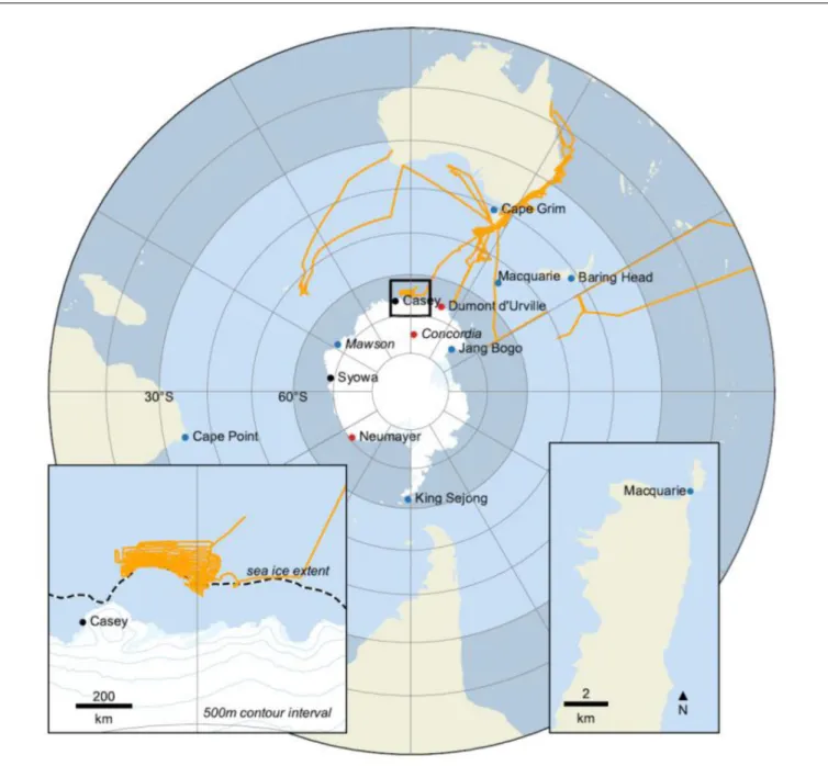
et al., 2002;Pereira et al., 2004;Brunke et al., 2004;Zahorowski et al., 2013; Chambers et al., 2014, 2017; Weller et al., 2014). Detection methods have included electrostatic deposition (Pereira and da Silva, 1989;Ui et al., 1998;Tositti et al., 2002), static single-filter detectors (Levin et al., 2002), and two-filter detectors (Chambers et al., 2014). Stations presently contributing to the Southern Ocean network of radon detectors include: Cape Grim (CG), Baring Head (BH), Cape Point (CP), Macquarie Island (MI), Jang Bogo (JBS), King Sejong (KSG), and Neumayer (NM) (Figure 1).

Sites and Equipment

This article summarizes radon and auxiliary observations (e.g., meteorology, trace gasses and aerosols) from four of the long- term ongoing monitoring stations in the Southern Ocean network (MI, KSG, NM, and JBS), as well as Dumont d’Urville (DDU), Dome Concordia (DC), and selected observations from the Research VesselInvestigator(Table 1). Brief mention is also made of previously published observations from Mawson Base (Chambers et al., 2014). All reported times are local station times. For RV Investigator and MI observations the standard Southern Hemisphere seasonal convention has been adopted. For the Antarctic bases “summer” refers to the period November through February, “winter” the period April through September;

March and October are considered transitional months.

The RV Investigator’s radon detector was installed in September 2014 in the Aerosol Sampling Laboratory at the bow of the vessel, immediately below the sampling mast on the foredeck.

Sample air is drawn at 65–75 L min⁻¹ from a goose-neck inlet at 15 m above the foredeck (around 20–22 m above sea level, a.s.l.) through 25 mm HDPE agricultural pipe. A coarse aerosol filter, dehumidifier and water trap are installed upstream of the detector, to protect the detector’s primary filter and internal components. Calibrations are performed on either a campaign or quasi-monthly basis by injecting radon from a PYLON Radon- 222 source (20.62±4% kBq²²⁶Ra, delivering 2.598 Bq min⁻¹

222Rn)¹ for 6 h at a flow rate of ∼100 cc min⁻¹, and the instrumental background is checked either on a campaign basis or every 3 months. Details of other atmospheric observations aboard the RVInvestigatorare given inProtat et al. (2016).

Macquarie Island is small (34×5 km), and is situated roughly midway between Australia and Antarctica (Figure 1). Radon and meteorological observations are made at the “Clean Air Laboratory” on an isthmus at the northern end of the island (∼54.5^◦S;Figure 1, inset 2). The MI radon detector was installed in March 2011, but technical problems delayed the start of the sampling program until March 2013. Sample air is drawn at

∼45 L m⁻¹ from an inlet∼5 m above ground level (a.g.l.) on a 10 m mast. The detector is calibrated monthly using a similar source to the RVInvestigator(19.58±4% kBq²²⁶Ra) injecting for 6 h at a flow rate of∼170 cc min⁻¹. Instrumental background checks are performed quarterly by stopping the internal and external flow loop blowers for 24 h. Further information about MI observations can be found inBrechtel et al. (1998)andStavert et al. (2018).

1https://pylonelectronics-radon.com/

(4)

FIGURE 1 |Southern Ocean radon detector network: two-filter detectors (blue), single-filter detectors (red). RV Investigator cruise track (January 2015 to June 2017) shown in orange. Inset 1 shows RV Investigator maneuvers for sea floor mapping (January–February 2017), and includes the February 2017 sea ice extent based on the 20% concentration contour from passive microwave satellite data (Peng et al., 2013;Meier et al., 2017). Ice sheet elevation contours are from ETOPO1 (Amante and Eakins, 2009). Inset 2 shows location of Macquarie Island monitoring station with coastline data from Natural Earth and, for the Macquarie Island inset, the Australian Antarctic Division (2005).

A similar protocol is followed for the two-filter detectors at KSG and JBS. For details the reader is referred to existing publications (Chambers et al., 2014, 2017). Further details about the regions surrounding KSG and JBS are given inEvangelista and Pereira (2002)andTositti et al. (2002).

Radon observations at NM, DDU, and DC were all made using single-filter (“by progeny”) Heidelberg Radon Monitors (HRM, Levin et al., 2002). The current system providing 3-hourly radon observations at Neumayer Station has been in place since 1995.

Specific details about the site as well as the setup and operation of the Neumayer HRM and other observations are provided in Weller et al. (2014). Specifically regarding the NM radon sampling inlet, ambient air is first sucked through 3 m of 200 mm electro-polished stainless steel at 8.8 m s⁻¹, then through 2.8 m of 50 mm electro-polished stainless steel tube at 2 m s⁻¹, and finally through∼50 cm of 6 mm stainless steel tube at 21 m s⁻¹.

At DDU the HRM was setup in laboratory “Labo 3” (e.g., Preunkert et al., 2012) in which other long-term atmospheric

(5)

TABLE 1 |Sites, detection method, time periods, and responsible organizations for observations discussed in this study.

Station/Platform Period of observations

Radon detector, responsible organizations and lower limit of detection

RV Investigator (ongoing)

January-2015 to June-2017

700L two-filter detector;

Australian Marine National Facility, CSIRO, ANSTO; LLD 40 mBq m⁻³

Macquarie Island (ongoing)

March-2013 to December-2016

Australian Antarctic Division (AAD), CSIRO, ANSTO; LLD 40 mBq m⁻³

King Sejong (ongoing) February-2013 to December-2016

Korea Polar Research Institute (KOPRI), ANSTO; LLD 25 mBq m⁻³

Jang Bogo (ongoing) January-2016 to December-2017

KOPRI, ANSTO; LLD 30 mBq m⁻³

Neumayer (ongoing) January-2010 to December-2011

Static single-filter detector;

Alfred Wegener Institute for Polar and Marine Research, University of Heidelberg (Institut für Umweltphysik); LLD 20 mBq m⁻³

Dumont d’Urville (terminated)

January-2006 to December-2008

University Grenoble Alpes (CNRS), University of Heidelberg (Institut für Umweltphysik); LLD 60 mBq m⁻³

Dome Concordia (terminated)

January-2010 to March-2011

University Grenoble Alpes (CNRS), University of Heidelberg (Institut für Umweltphysik); LLD 60 mBq m⁻³

Mawson (terminated) January-1999 to August-2000

Australian Antarctic Division (AAD), ANSTO; LLD∼50 mBq m⁻³

measurements such as ozone (Legrand et al., 2009, 2016), sulfur species (Preunkert et al., 2008), gaseous elemental mercury (GEM, 2012–2015; Angot et al., 2016c; Sprovieri et al., 2016), other aerosols and reactive gasses are also conducted. The radon measurement resolution was hourly and sampling was more direct than at NM, simply through ∼4 m of 6 mm diameter Teflon tubing from 2 m a.g.l. In all other respects the HRM and its operation were as for NM. The DC HRM was situated in the main building of the station. The device was also set to sample hourly, through∼4 m of 6 mm diameter Teflon tubing, but at a height of 17 m a.g.l., and run in parallel to long-term measurements of aerosols, SO2 (Legrand et al., 2017a,b) and ozone (Legrand et al., 2009, 2016) as well as GEM (Angot et al., 2016b). In all other respects, the HRM instrument and operation were as for NM.

Specifically regarding the two-filter detectors, both the 700 and 1500 L models have a response time of ∼45 min (which can

be corrected for in post-processing; Griffiths et al., 2016), and their response to even very low radon concentrations (<100 mBq m⁻³) is linear. Their lower limits of detection (LLD; i.e., the concentration at which the detector’s counting error reaches 30%) are∼25 mBq m⁻³ and∼40 mBq m⁻³, for the 1500 and 700 L models, respectively. Their measurement error is typically 12–

14% for concentrations of 100 mBq m⁻³(Chambers et al., 2014;

Schmithüsen et al., 2017). This uncertainty is contributed to by the counting error, the coefficient of variability of monthly calibrations, and the calibration source uncertainty. The counting error’s contribution reduces with increasing radon concentration and, when sampling from a consistent fetch, the detector’s measurement error reduces as∼N⁻^1/2 for N samples. For the purposes of this study the half-hourly raw counts from each detector were integrated to hourly values before calibration to activity concentrations (mBq m⁻³), thereby reducing the counting error by a factor of√

2.

The two-filter method detects radon by zinc sulfide alpha scintillation, which does not distinguish between alpha particles of different energies, so a∼5 min delay volume is incorporated within every detector’s inlet line to allow the short-lived radon isotope (²²⁰Rn, thoron, t_0.5= 56 s) to decay to less than 0.5%

of its ambient values before sample air enters the detector.

Radon concentrations provided by some “direct” methods (e.g., two-filter detectors or electrostatic deposition detectors;Pereira and da Silva, 1989; Wada et al., 2010; Grossi et al., 2012) are not adversely influenced by high ambient humidity or changing aerosol loading conditions, proximity to local sources, atmospheric stability or fetch conditions. In a possible exception to this however, under low humidity conditions (i.e., 0–20%;

common during Antarctic winters when cold ambient air is brought to detector temperature), the two-filter method can theoretically report concentrations up to 10% below ambient values due to a reduction in diffusivity, and consequent lower filtration efficiency, of the unattached progeny formed inside the detector (Griffiths et al., 2016). However, this effect is counteracted by reduced losses in the delay tank of the detector, and no significant evidence of a reduced detector sensitivity to radon concentrations was found based on 2 years of monthly calibrations of the Antarctic two-filter detectors over relative humidity values between 5 and 45%.

Specifically regarding the HRMs (single filter detectors), a correction factor of 1.11 has been applied to observations from all three sites to better harmonize their radon concentrations with the two-filter detector observations (as recommended by Schmithüsen et al., 2017). The radon disequilibrium correction discussed by Schmithüsen et al. (2017) is not required for the NM or DC observations due to the lack of significant local radon sources. Similarly, under oceanic fetch conditions at DDU no disequilibrium correction is required. For DDU observations under other fetch conditions a disequilibrium factor of 0.85–

0.9 would be applicable to radon contributions from local fetch regions. However, since the relative contributions of local and remote radon sources to DDU observations under other fetch conditions are uncertain, no disequilibrium factor was applied to results presented. Although a large fraction of the hourly DDU and DC radon observations were below the LLD reported in

(6)

Table 1, the uncertainty of monthly mean/median values, and diurnal composites by season, reduces as∼N⁻^1/2for N hourly samples. Finally, as noted by Levin et al. (2017), “tube loss”

of ambient radon progeny can reduce HRM radon estimates, particularly under very low ambient radon concentrations as is typical of the Antarctic atmosphere. We were unable to accurately characterize the magnitude of this influence on the NM, DDU and DC radon observations, but it is believed to have contributed in part to reported mean radon concentrations 10–15 mBq m⁻³ lower than those of the two-filter detectors under similar fetch conditions.

RESULTS

The Southern Ocean in Cross-Section

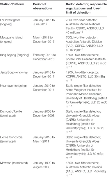
During the initial 2.5 years that radon was measured aboard the RV Investigator the vessel completed five full crossings of the Southern Ocean between the latitudes 45^◦S and 67^◦S, including a month of maneuvres near the Antarctic coast to the east of Casey Station for sea floor mapping (Figure 1). Since all transects were conducted in months between January and April they are representative of warmer conditions for this region. To demonstrate the utility of radon as a tracer of recent terrestrial influence, and provide a late-summer cross-section “snapshot” of potentially polluted air masses within the Southern Ocean’s MBL, we prepared a composite of mean radon concentrations within 0.2^◦latitude bins (Figure 2A). This figure constitutes a significant improvement to transects reported by Polian et al. (1986) at 2–3 degree resolution, or the daily ship-based measurements reported by Taguchi et al. (2013), and provides context for measurements at the fixed sites discussed in the following sections.

Between 49–51^◦S and 62–64^◦S average radon concentrations were close to 50 mBq m⁻³, indicative of minimal terrestrial influence within the past 2–3 weeks (i.e., marine “baseline”

values, with radon in equilibrium with the Southern Ocean surface; Crawford et al., 2018 and references therein). By comparison, near the middle of this composite transect (i.e., 53–56^◦S) an enhancement of 30–40 mBq m⁻³ above baseline conditions was observed. Some previous studies have hypothesized that enhanced radon in the mid-Southern Ocean is entirely attributable to a wind-speed induced increase in the oceanic radon flux (e.g., Schery and Huang, 2004;

Zahorowski et al., 2013). However, more recent evidence from an initial comparative baseline analyses of Cape Grim (Tasmania) and Macquarie Island air masses (Williams et al., 2017), suggests this radon enhancement is largely attributable to vestigial terrestrial influences on mid-Southern Ocean air masses. A detailed evaluation of this hypothesis will be the subject of a separate investigation. Notable similarities between Figure 2Aand earlier transects reported byPolian et al. (1986) include higher concentrations around 60^◦S and at the Antarctic coast, with a local minimum in concentration around 63–

64^◦S.

Several examples of isolated radon excursions from otherwise background conditions are evident inFigure 2A (e.g., at 46.5,

52.5, and 56.5^◦S). Back trajectories (HYSPLIT v4.0,Draxler and Rolph, 2003; using GDAS wind fields) indicated that contributing events were attributable to low-level (MBL) synoptic transport from Australia or New Zealand (e.g.,Figure 3).

The corresponding Southern Ocean CO₂transect (Figure 2B) shows enhancements associated with each of the three synoptic transport events identified in the radon record. Of equal interest, however, is the structure evident in the composite CO2transect that is not associated with recent terrestrial influence (e.g., Stavert et al., 2018). This demonstrates the utility of high- quality shipborne radon observations in helping to isolate CO₂ contributions arising from oceanic processes, terrestrial influences in excess of 3-weeks old or shipping exhaust.

A broad region of enhancement in both radon and CO2 is evident between 59 and 61^◦S. Back trajectories corresponding to the largest of these events (not shown) were not associated with synoptic MBL transport events, but were found to have recently descended from above the MBL. A mechanism for such transport events, postulated by Humphries et al. (2016), is terrestrially influenced free tropospheric air subsiding or intruding into the MBL in the vicinity of the circumpolar trough (“Polar Front”). This may provide further insight to high particle concentration events observed previously in the region (e.g., Humphries et al., 2015, 2016). Decay-correcting the observed radon concentrations based on modeled tropospheric transport times may provide a means of constraining the magnitude of the original terrestrial influence on the tropospheric air mass.

The last pronounced feature ofFigure 2Ais a “ramping” of radon concentration between 64 and 67^◦S (over∼350 km). This increasing terrestrial influence on MBL air masses approaching the Antarctic coast in summer-autumn is attributable to two separate influences: a local Antarctic radon contribution from coastal exposed rocks (Evangelista and Pereira, 2002; Taguchi et al., 2013;Burton-Johnson et al., 2016;Chambers et al., 2017), and a remote terrestrial contribution within the outflow of tropospheric air masses that are descending over the Antarctic continent (Polian et al., 1986;Chambers et al., 2014, 2017). The fact that there is a step increase in CO₂ within this same zone indicates that the outflow of subsiding tropospheric air is a large contributing factor, as the CO2 increase likely represents air that has not been in recent contact with the oceanic CO₂ sink (Stavert et al., 2018). The ramping of radon concentrations may be partially a result of radioactive decay, indicating that the net northward movement of these outflowing air masses is quite slow (as expected of the strong easterly flow south of the circumpolar trough).

Seasonality of Terrestrial Influence in the Mid-Southern Ocean

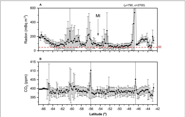
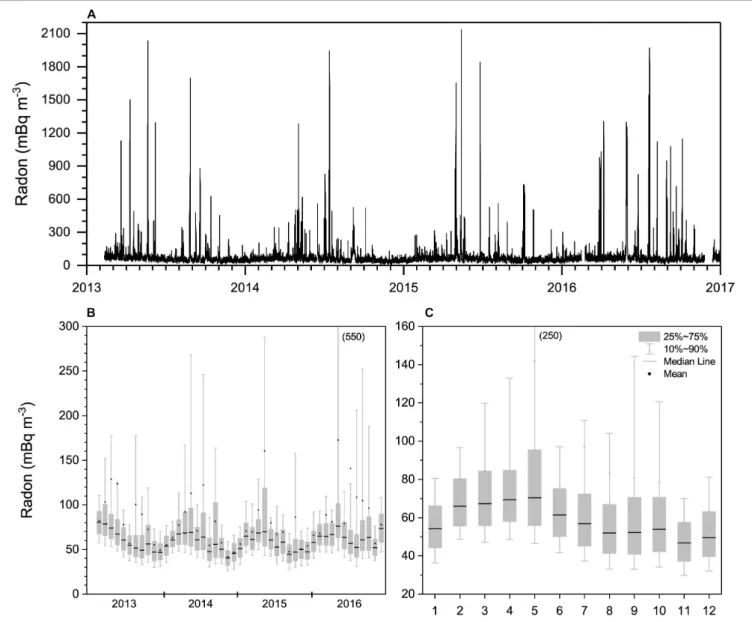
Despite the isolation of MI (2000 km from mainland Australia, 1500 km from Tasmania, 1000 km from New Zealand), high radon concentrations (1500–3000 mBq m⁻³) were observed on average 4 times a year. Based on the conditions necessary to measure a significant (≥200 mBq m⁻³) local influence, i.e., a wind sector of 180–270^◦ (Figure 1, inset 2) and wind

(7)

FIGURE 2 |5-track composite of(A)radon, and(B)carbon dioxide, concentrations (0.2^◦latitude bin means) between 45 and 67^◦S of Southern Ocean MBL.

Whiskers represent±1σ. Approximate location of Macquarie Island is marked.

FIGURE 3 |Back trajectories,(A)x-y and(B)x-z projections, associated with a mid-Southern Ocean radon enhancement event originating from south eastern Australia observed by the RVInvestigator. Typical height range of the mid-Southern Ocean marine boundary layer inversion indicated.

speeds < 10 m s⁻¹, less than 0.5% of events > 200 mBq m⁻³ in Figure 4A could be attributed to local island influences. When compared to radon in air masses leaving

mainland Australia (50th – 75th percentile events 2000–

4000 mBq m⁻³; Zahorowski et al., 2013), this indicates that it is possible for terrestrially influenced air masses

(8)

FIGURE 4 | (A)Hourly, and(B,C)monthly distributions of radon concentrations at Macquarie Island based on a 4-year (2013–2016) composite of hourly observations. Refer to key for distribution box-plot details.

to travel far into the Southern Ocean without substantial dilution.

Monthly means and distributions of radon (Figures 4B,C) indicated a pronounced seasonal cycle characterized by a winter maximum and summer minimum. This cycle is thought to be largely attributable to the seasonal migration (north in winter, south in summer) of the surface divergence zone between the Hadley and Ferrel Cells (the “Subtropical ridge”), the average position of which is ∼30^◦S (see Figure 5 ofDoering and Saey, 2014; Williams et al., 2017). Back trajectories calculated by Williams et al. (2017) indicated that even the seasonal cycle in the 10th percentile values is caused by vestigial continental influences.

To investigate possible wind speed influences on mid- Southern Ocean radon concentrations we calculated monthly wind speed distributions (not shown). The seasonal cycle, characterized by a broad March–October maximum

(monthly median wind speeds of 10.3–11.3 m s⁻¹) and November–February minimum (monthly median wind speeds 8.8–10.3 m s⁻¹), had a low amplitude and did not match well with the seasonal radon cycle. Clearly, the seasonality of wind speed at this site is not the dominant influence on the seasonality in MBL radon concentrations.

Mean summer-autumn radon in the RV Investigator data at 54.5^◦S (Figure 2A) was 90–100 mBq m⁻³. This agrees well with the January–April monthly mean MI radon concentrations (Figure 4A). Agreement of mean concentrations within ∼10 mBq m⁻³ (i.e., ∼10%) between independently calibrated two-filter detectors provides confidence in comparisons drawn between other two-filter detectors in the Southern Ocean Network. Further confidence in the absolute radon concentrations reported by the RV Investigator is given by the estimate of 50 mBq m⁻³ for MBL air masses in the 49–51^◦S region of the Southern

(9)

Ocean, as also reported by the independently operated 5000 L radon detector (LLD < 10 mBq m⁻³) at Cape Grim Station, Tasmania (Williams et al., 2017; Crawford et al., 2018).

It has already been demonstrated (Figure 2A) that minimum MBL radon concentrations in summer-autumn are higher toward the middle of the Southern Ocean than around 49 or 63^◦S.

In addition, Figure 4C demonstrates that the magnitude of this enhanced terrestrial influence in the Southern Ocean varies seasonally, and is largest in winter.

Approaching the Antarctic Coast

In late summer 2017 (20-January to 25-February) the RV Investigator conducted a sea floor mapping exercise 200 – 400 km east of Casey Station, between about 50 and 150 km off the Antarctic coast (Figure 1, inset 1). Periods of considerable variability in trace atmospheric constituents and cloud condensation nuclei (CCN; TSI CPC Model 3776, size range>3nm) were observed during this voyage. We investigate here whether they could be attributed to similar processes as the free-tropospheric particle events observed near the circumpolar trough (“Polar Front”) byHumphries et al. (2015, 2016).

This far offshore, little diurnal variability in MBL depth or radon concentration was expected given the ocean’s heat capacity, and the fact that the open ocean is a weak radon source without a diurnal cycle (Schery and Huang, 2004; Zahorowski et al., 2013), respectively. Over the course of the 37-day mission, however, amplitudes of the radon diurnal cycle varied from 0 to 50 mBq m⁻³(Table 2). The amplitudes reported inTable 2were calculated as the difference between 5-h means centered on the daily maximum and minimum hourly values.

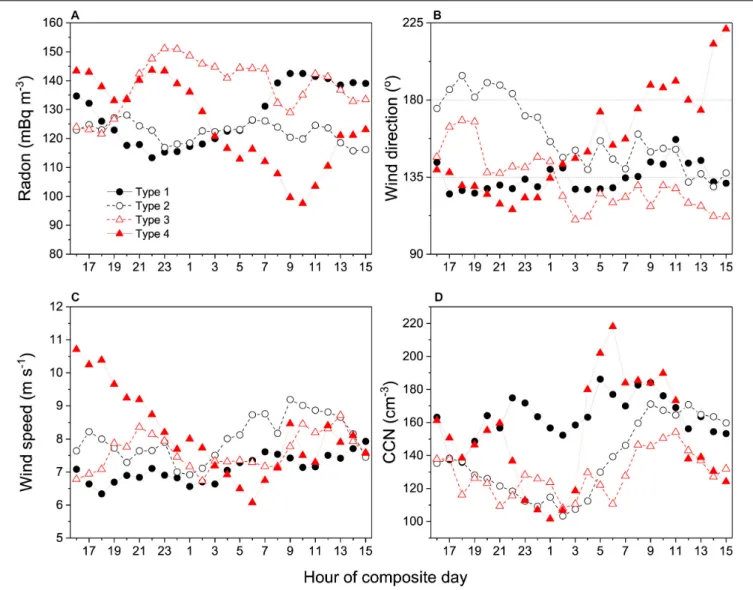
On some days the diurnal cycle was characterized by a daytime maximum and on others a nocturnal maximum (Table 2; Figure 5A). While the magnitudes of these diurnal cycles are 2–3 orders of magnitude lower than typically found at inland terrestrial sites (e.g., Chambers et al., 2015), the absolute accuracy of the two-filter detectors (<12% on a 1-h count for Rn > 100 mBq m⁻³; see Sites and Equipment), nevertheless provides confidence in the observed differences discussed below. Specifically, the uncertainty on each diurnal cycle amplitude (DU) is twice the uncertainty of the daily maximum or minimum estimate (^12%^√

5 =5.4%); i.e., DU = 2(5.4%) = 10.8% ≈ 14 mBq m⁻³. While this level of uncertainty can’t guarantee clear distinction between type 2 and 3 events in Table 2, it is sufficient to distinguish type 1 and type 4 events, and each of these events from either type 2 or 3.

Type 1 days were characterized by daytime radon around 140 mBq m⁻³(Figure 5A), wind directions from the southeast (Figure 5B; along the local coastline, Figure 1 inset 1), relatively consistent wind speeds (Figure 5C), and no pronounced diurnal cycle in CCN (Figure 5D). In this case the radon diurnal cycle amplitude (Rn_AMP = 25 mBq m⁻³) is likely attributable to changes in the coastal radon source function related to the diurnal freeze-thaw cycle, and this coastal air mixing to the local MBL (e.g., Bromwich et al.,

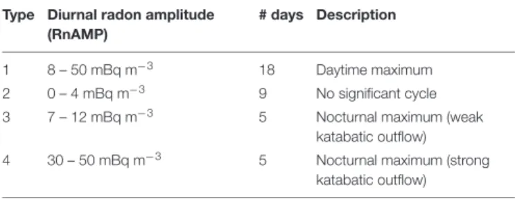
TABLE 2 |Daily summary of MBL radon concentration characteristics observed from the RVInvestigatorbetween 20-January and 25-February 2017.

Type Diurnal radon amplitude (RnAMP)

# days Description

1 8 – 50 mBq m⁻³ 18 Daytime maximum

2 0 – 4 mBq m⁻³ 9 No significant cycle

3 7 – 12 mBq m⁻³ 5 Nocturnal maximum (weak

katabatic outflow)

4 30 – 50 mBq m⁻³ 5 Nocturnal maximum (strong

katabatic outflow)

1993). The January mean daily maximum and minimum coastal temperatures at Casey were +2.3 and −2.5^◦C, respectively.

Type 2 days had no consistent radon diurnal cycle and wind directions that changed from southerly to south-easterly, consistent with the passage of cyclonic synoptic systems. On overcast summer days coastal air temperatures typically peaked between −2 to 0^◦C, leading to less of a change in the coastal radon source function. Indeed, diurnal mean radon on these days was similar to the nocturnal concentrations for Type 1 days.

The diurnal course of CCN on Type 2 days seemed to closely correspond to diurnal changes in wind speed and direction (oceanic fetch is more recent for south easterly air masses), indicating that salt spray was likely a dominant component of these aerosols.

Type 4 days were characterized by Rn_AMP = 46 mBq m⁻³, with a late morning minimum (Figure 5A). Until shortly after midnight the wind direction was roughly parallel to the coast and wind speeds were decreasing. From 0100 to 0200 h wind direction swung round to the south and southwest, almost perpendicular to the local coastline, and wind speeds increased by ∼3 m s⁻¹. During this period, CCN increased to values higher than observed under the windiest conditions of Type 2 days, indicating that their origin is unlikely to relate to sea spray. Type 3 days shared many characteristics with Type 4 days, but to a lesser degree (reduced morning radon minimum, smaller and delayed morning peak in CCN).

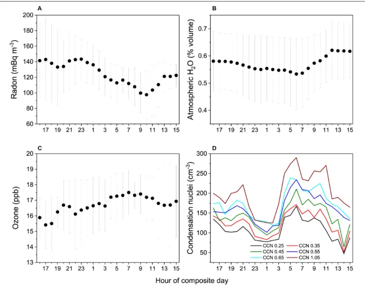
In Figure 6 we investigate Type 4 days in more detail.

Radon variability in the offshore flow (0400–1100 h) was lower than for periods of alongshore flow (Figure 6A). Air masses associated with offshore flow were also drier (Figure 6B). Ozone concentrations from 0400 to 1100 h were higher and less variable, and an increase was observed in all supersaturation ranges (0.25 – 1.05%) of CCN. The combination of timing, wind direction and air mass humidity suggest these morning events on Type 4 days are associated with katabatic outflow from the Antarctic mainland.

Since air within Antarctic katabatic flow events originates in the free-troposphere (Nylen et al., 2004), and crosses the coast at right angles (rather than traveling along or obliquely to it), there is a reduced opportunity for fetch across exposed rock, thereby reducing the average radon enhancement above

“background” levels (30–50 mBq m⁻³) during outflow events.

(10)

FIGURE 5 |Diurnal composite(A)radon (means),(B)wind direction (medians),(C)wind speed (means), and(D)CCN (means across all supersaturation ranges; see Figure 6D), as observed from the RVInvestigatorfor each day type described inTable 2. Time axis shifted to focus on the nocturnal period.

Having originated from the free-troposphere, these air masses also start out considerably drier than MBL air masses, and with higher ozone content. With their origin in mind, the observed increase in CCN of these recently tropospheric air masses is likely attributable to sulfate influences in the free-troposphere (Humphries et al., 2016;Obryk et al., 2018). In these regions the sulfate could be of anthropogenic, marine or volcanic origin (Graf et al., 2010). Related to these observations,Jaenickle et al. (1992) also reported an increase of CCN in subsiding tropospheric air at Neumayer station. As expected, back trajectories (not shown) confirmed that the free-tropospheric contributions to MBL air between 0400 and 1100 h on the outflow days of this study did not derive from the same tropospheric injection processes as those described by Humphries et al.

(2016).

Five strong katabatic events in 37 days (Table 2), a relative frequency of∼14%, is very similar to the 12% event frequency of pronounced katabatic flow in summer at Jang Bogo station

reported by Chambers et al. (2017). The timing of the peak outflow was delayed by about 3 h compared to that of coastal events reported by Chambers et al. (2017), but this can be attributed to travel time based on the vessel’s distance from shore and the observed mean wind speeds of 8–9 m s⁻¹.

The relatively weak contrasts in radon and humidity between katabatic outflow and MBL air masses shown inFigures 6A–C compared to the results ofChambers et al. (2017)and Section

“Continental Antarctica” below indicate that considerable mixing (or ocean-atmosphere exchange) of the outflow air mass has occurred in transit to the RV Investigator. While this mixing prevents the reliable characterisation of tropospheric air in the outflow events in the way that can be achieved at coastal Antarctic sites (see Continental Antarctica), our findings clearly demonstrate that shipborne aerosol and trace gas measurements near the Antarctic coast should separately treat katabatic outflow days, or consider diurnal sampling windows, since the characteristics of recently tropospheric

(11)

FIGURE 6 |Diurnal composites of(A)radon,(B)% volume of water,(C)ozone, and(D)CCN (cm⁻³) within supersaturation ranges 0.25 – 1.05%, based on 5 days of katabatic outflow conditions. Whiskers represent hourly±1σfor the 5 days composite.

outflow air masses (i.e., potentially containing remote terrestrial influences) will not be representative of local conditions and may temporarily modify local ocean-atmosphere exchange processes.

Continental Antarctica

Coastal Sub-Antarctic (King Sejong Station: 62.2^◦S) King Sejong Station is among the northernmost of the Antarctic bases (Figure 1), being about 500 km further north than most of the Antarctic coastline. Since the station is well removed from the topographic influences of the East Antarctic ice sheet, which reaches elevations above 4000 m a.s.l., of the Antarctic bases in this study KSG is best suited for year-round characterisation of marine baseline air masses of the remote Southern Ocean. In addition, the tip of the Antarctic Peninsula is also closer than any other part of continental Antarctica to another Southern Hemisphere continent (South America), so it also provides

unique opportunities to observe the influence of recent direct transport of natural and anthropogenic terrestrial emissions to the frozen continent (e.g., Pereira, 1990; Pereira et al., 2004;

Chambers et al., 2014).

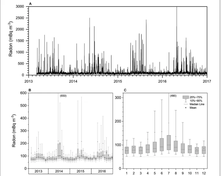
Peak KSG radon concentrations (1500–2000 mBq m⁻³; Figure 7A) were lower than at MI, despite KSG being closer to South America than MI is to Australia. This is attributable to the combination of limited land fetch across South America (Pereira, 1990;Chambers et al., 2014), and high soil moistures in southern Chile.

Summer median KSG radon concentrations were 50–55 mBq m⁻³ (Figures 7B,C), similar to the minimum 0.2^◦ latitude bin mean values reported for this zone by the RV Investigator (Figure 2A), but lower than the corresponding MI values (75–

80 mBq m⁻³; Figure 4C). This difference provides further independent confirmation of the small mid-Southern Ocean radon enhancement observed in the RVInvestigatorcomposite transect (Figure 2A). It should be noted here that, due to the

(12)

FIGURE 7 | (A)Hourly, and(B,C)monthly distributions of KSG radon concentrations between 2013 and 2016. Refer to key for distribution box-plot details.

station’s location (see Chambers et al., 2014), many KSG air masses with extensive oceanic fetch have to traverse at least

∼2 km of King George Island before reaching the site. Based on typical radon fluxes, mixing depths and wind speeds reported in Chambers et al. (2014), this terrestrial influence could enhance oceanic fetch radon concentrations by 5–10 mBq m⁻³.

The KSG radon seasonal cycle (Figures 7B,C) was quite distinct from that at MI. While minimum values were observed at both sites between November and January, peak values at KSG were bimodal, occurring in March-May and September–

October. The latitude of KSG is close to the mean location of the circumpolar trough (convergence zone between the Ferrel and Polar Cells). Consequently, the seasonal migration of the circumpolar trough results in KSG switching between the influence of mid-latitude westerlies and Polar easterlies. In the non-summer months the synoptic cyclone track within the circumpolar trough is well located to bring air masses from the tip

of South America to the station (Pereira et al., 2006and references therein;Chambers et al., 2014).

Coastal Antarctica Dumont d’Urville (66.7^◦S)

Two of the RVInvestigatortransects summarized in Section “The Southern Ocean in Cross-Section” approached the Antarctic coast near Dumont d’Urville (Figure 1). Inland from DDU the elevation reaches 2000 m a.s.l. within 200 km, before continuing up to >4000 m a.s.l. at the highest point of the Antarctic Plateau. Consequently, DDU is ideally situated to separately characterize long-term Southern Oceanic MBL air masses, as well as tropospheric air that has recently subsided over the Antarctic Plateau and comes down as katabatic flow events.

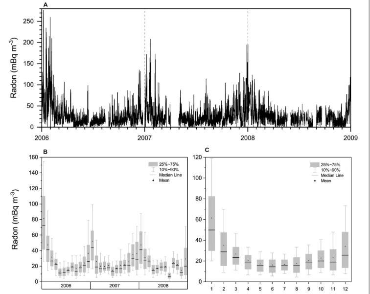
Peak DDU radon concentrations (180 – 275 mBq m⁻³; Figure 8) were an order of magnitude less than MI or KSG values,

(13)

FIGURE 8 | (A)Hourly, and(B,C)monthly distributions of DDU radon concentrations between 2006 and 2009. Refer to key for distribution box-plot details.

presumably because the nearest upwind non-frozen terrestrial fetch is 2500 – 3000 km away. However, the seasonal DDU radon cycle reported here (18 – 61 mBq m⁻³, based on monthly means), was also less than that reported byPolian et al. (1986) for DDU (25 – 65 mBq m⁻³), and less than the seasonal cycle at Mawson (67.5^◦S) (30 – 130 mBq m⁻³;Chambers et al., 2014).

Furthermore,Ui et al. (1998)reported spring-summer daily mean radon concentrations at the coastal station of Syowa (69^◦S) between 150 and 270 mBq m⁻³. Potential factors contributing to this discrepancy have been discussed in Section “Sites and Equipment.”

Similar to MI, the seasonal DDU radon cycle was unimodal, although peak concentrations occurred in mid-summer (Figure 8). Three factors are thought to have contributed to the summer increase in DDU radon concentrations: (i) the southward shift of the circumpolar trough permits passing cyclonic weather systems to bring air containing vestigial terrestrial influences from deeper within the Southern Ocean

MBL directly to DDU; (ii) a greater amount of exposed rock and shallow coastal water at this time gives rise to an increased local radon flux from land and ocean; and (iii) tropospheric air descending over Antarctica in summer typically has experienced more recent terrestrial influence than corresponding winter air masses.

To further investigate these possible influences we employed a recently developed technique to separate air masses of different fetch at coastal East Antarctic sites (see Section 3.5 ofChambers et al., 2017). Here, the multi-year dataset was analyzed in 24-h blocks (defined from 1400 h to 1300 h the following day), each of which were assigned a category of “katabatic,”

“local” or “oceanic” based on the mean 2-week high-pass filtered absolute humidity within an 8-h window (0000–0700 h) typically associated with katabatic flow. Days with the lowest 20% absolute humidity over this 8-h window are most likely to have experienced katabatic flow events. Days with the highest 20% absolute humidity over this 8-h window have experienced

(14)

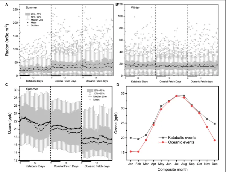
FIGURE 9 |Diurnal composite(A,B)radon, and(C)ozone distributions, for days containing periods of katabatic, coastal and oceanic fetch at DDU, based on absolute humidity in the window 0000–0700 h (see text and plot key for details);(D)comparison of monthly mean ozone in katabatic and MBL air masses, at DDU based on observations from 2006 and 2008.

the most consistent oceanic fetch (i.e., arrived at the site most directly from the ocean). All remaining days (60% of the observations) were placed in the “coastal fetch” category (Figures 9A,B). Since the technique relies upon a measure of absolute humidity to assess fetch categories, as opposed to wind speed and direction or other meteorological quantities, it is capable of distinguishing between downslope flow that is truly katabatic, and downslope flow that has been synoptically forced.

While results are presented here as full diurnal composites (0000 – 2300 h), the fetch analysis described above only strictly applies to the 0000–0700 h diurnal window, which has been marked with a bold line on each plot. Across the edges of the 24-h compositing window (i.e., between and close to the hours 1300–1400 h), discontinuities can arise due to edge effects of the compositing process (e.g., Figure 9C). Wind direction for oceanic fetch within the 8-h window was 110–120^◦and changed to 140–150^◦under katabatic conditions.

The highest mean DDU radon concentrations in summer (45–50 mBq m⁻³) occurred under oceanic fetch conditions (Figure 7A, RHS), consistent with expected radon concentrations for air in equilibrium with the Southern Ocean surface (30–50 mBq m⁻³; Zahorowski et al., 2013; Chambers et al., 2016). Outlier values of 90 – 265 mBq m⁻³ for these events indicate that oceanic air masses occasionally exhibit a vestigial terrestrial influence, likely attributable to long-range synoptic transport within the MBL (though possibly also related to subsidence near the circumpolar trough, see The Southern Ocean in Cross-Section).

On summer days, when coastal fetch prevailed in the 0000–0700 h diurnal window, mean radon concentrations were slightly lower (40–45 mBq m⁻³; Figure 9A, center), despite median values for oceanic and coastal events being almost identical. The reduced skewness of coastal events (90th percentile concentrations of 75–90 mBq m⁻³ compared with

(15)

FIGURE 10 |Diurnal composite(A)wind speed,(B)gaseous elemental mercury, and(C)ultraviolet radiation, at DDU (January-2012 to May-2015).

95–100 mBq m⁻³for oceanic events), is consistent with coastal events receiving low radon contributions from small, local coastal sources as discussed by Evangelista and Pereira (2002) and Chambers et al. (2014, 2017).

The lowest mean DDU radon concentrations in summer (24–29 mBq m⁻³) were associated with katabatic drainage events (from the free-troposphere/Antarctic Plateau). Unlike boundary layer air masses, free-tropospheric air masses have had an opportunity to be removed from all radon sources (terrestrial or oceanic) for a period of time, enabling them to achieve radon concentrations below even the 30–50 mBq m⁻³ associated with clean marine air. However, 10% of katabatic flow events (the marked outliers in Figure 9A, LHS) had radon concentrations between 55 and 165 mBq m⁻³, suggesting terrestrial influence within the past 2–3 weeks (ignoring dilution within the troposphere). Vertical profiles near DDU reported by Polian et al. (1986) also indicated an increase in radon concentrations from∼15 mBq m⁻³near the surface to∼80 mBq m⁻³between 2000 and 3000 m a.s.l., which is near the elevation of genesis for katabatic flow.

In summer there is∼600 m of partially-exposed (∼50%) rock and soil to the south (inland) of DDU station (Preunkert et al., 2012). At speeds typical of katabatic flow (6–12 m s⁻¹, gusting to 23 m s⁻¹), even assuming a large radon flux (20 mBq m⁻² s⁻¹), and shallow mixing depths for these wind speeds (∼100 m), it is very unlikely that this fetch could contribute more than 10–

15 mBq m⁻³to the observed concentrations in the katabatic flow.

Consequently, the bulk of the signal must arise from terrestrial influences within the tropospheric air.

Contrary to the summer results, the highest mean DDU radon concentrations in winter (Figure 9B) were in the katabatic flow events (18–21 mBq m⁻³; 27% lower than corresponding summer events). Peak concentrations of the winter katabatic events were 35–80 mBq m⁻³, indicating a summer-winter reduction in terrestrial influence on tropospheric air over DDU of almost a

factor of two. Median winter radon concentrations of coastal and oceanic events were the same (∼16 mBq m⁻³), although mean values of the events coming most directly from the ocean were around 10% higher. The lower concentrations for coastal events are likely attributable to a greater air mass fetch time over ice, from which no radon is emitted, rather than open ocean, as previously mentioned byWeller et al. (2014)for radon observations at Neumayer Station. Based on baseline radon concentrations of 30–50 mBq m⁻³, and the 3.8-day radon half- life, winter “oceanic” DDU air masses have likely spent 4–6 days traveling over ice.

To demonstrate the ability of this technique to separately characterize dominant fetch regions of coastal Antarctic air masses, we briefly investigate some other DDU trace atmospheric constituents. Figure 9C compares diurnal composite summer ozone concentrations for katabatic, coastal fetch, and oceanic fetch days. Within the 8-h analysis window mean summer ozone concentrations were highest in katabatic flow (from the Antarctic Plateau) and lowest under oceanic fetch conditions.

The diurnal cycle of ozone at DDU was largest for days that experienced morning katabatic flow events (Figure 9C). The amplitude of this cycle was 2 (3) ppb based on hourly means (medians). These days typically experienced high radiation levels (e.g., Figure 10C) and lower mean wind speeds when averaged over the entire diurnal cycle. The ozone cycle was characterized by a mid-afternoon minimum and an early morning maximum at the time of peak katabatic flow, as evident in Figure 10A (black filled circles). Conversely, no consistent diurnal cycle was evident under oceanic fetch conditions (excluding the edge effect of the diurnal compositing procedure in the early afternoon).

On coastal fetch days the amplitude of the diurnal ozone cycle was smaller, with the morning peak occurring a few hours later (Figure 9C, middle). Based on back trajectory fetch analyses Legrand et al. (2016)also found that ozone concentrations of air masses arriving at DDU in summer from the Antarctic interior

(16)

FIGURE 11 | (A)Three-hourly, and(B,C)monthly distributions of NM radon concentrations for 2010 and 2011. Refer to key for distribution box-plot details.

were higher than those of oceanic air masses, in some cases by up to 10 ppbv.

We calculated the daily mean ozone concentrations each month (using only observations within the 8-h analysis window) for katabatic flow and oceanic fetch events and prepared a 3-year composite (Figure 9D). In the summer months (November–

February) we found that air descending from the Antarctic Plateau in katabatic flow events had monthly mean ozone concentrations around 5 ppb higher than oceanic air masses. The difference was much lower for the remainder of the year, but the tropospheric concentrations were always higher than those of oceanic air masses.

We processed a separate set of GEM observations at DDU (January-2012 to May-2015) in the same way to separate katabatic flow and oceanic fetch events (Figure 10). Mindful of possible temperature or UV-related GEM production in the coastal Antarctic environment (Angot et al., 2016c;Bargagli, 2016), we

looked at the difference between summer mercury concentrations of katabatic flow and oceanic fetch events when UV levels were lowest (2300–0300 h;Figure 10C). We found that the katabatic flow was depleted around 0.3 ng m⁻³ in GEM compared to long-term oceanic air masses. This difference is of the same sign, but larger in magnitude, than that initially reported by Angot et al. (2016b) based on a back trajectory method of katabatic flow event identification. Based on estimated values of GEM in the Antarctic free troposphere of 0.9–1.0 ng m⁻³ [see Antarctic Plateau (Dome Concordia: 75^◦S, 3,233 m a.s.l.); andSong et al., 2018], the recently free-tropospheric katabatic flow events must have incorporated a large amount of air from the Antarctic Plateau where nocturnal GEM concentrations in summer are relatively depleted [Antarctic Plateau (Dome Concordia: 75^◦S, 3,233m a.s.l.); andAngot et al., 2016c].

The higher GEM concentrations in oceanic air at DDU are consistent with a combination of natural (including oceanic,

(17)

FIGURE 12 | (A,B)Comparison of summer and winter diurnal composite radon distributions for katabatic, coastal and oceanic fetch, and(C,D)diurnal composite summer temperature and absolute humidity values for katabatic, coastal and oceanic fetch at NM in 2010 and 2011. Refer to key for distribution box-plot details.

especially in summer and fall) and anthropogenic sources of this long-lived (∼1 year residence time;Bargagli, 2016) gas. However, our estimated summertime oceanic GEM concentrations at DDU of ∼0.86 ng m⁻³ were slightly lower than summer concentrations reported at Troll Station (235 km inland of the Antarctic coast; 0.9 – 1.1 ng m⁻³), or at Italian Antarctic Station, Terra Nova Bay (74^◦41⁰S; 164^◦07⁰E) (0.9 ± 0.3 ng m⁻³) (Sprovieri et al., 2002, 2010; Dommergue et al., 2010), or Amsterdam Island (∼1.0 ng m⁻³) (Angot et al., 2014;

Slemr et al., 2015; Sprovieri et al., 2016), consistent with observations at Cape Grim (Tasmania) and Singleton (NSW) (Slemr et al., 2015; Howard et al., 2017), but higher than reported by Kuss et al. (2011)for the southern Atlantic Ocean (0.72 ng m⁻³).

Neumayer (70.6^◦S)

Neumayer differs from most coastal Antarctic stations in that, instead of being built on rock, the station sits on the Ekström Ice Shelf, away from potential local sources of radon. Peak 3-hourly radon concentrations at Neumayer (110 – 155 mBq m⁻³; Figure 11A) were lower even than observed at DDU.

While tempting to attribute these events to transport from South America, Weller et al. (2014) found little evidence for this.

Rather, trajectory analyses often traced the origins of these events to the Antarctic interior. Ui et al. (1998) also reported high radon at Syowa station associated with southerly winds (from the Antarctic interior) and lower wind speeds (characteristic of anticyclonic conditions), but attributed this – we believe incorrectly – to unidentified local sources.

As for KSG the NM seasonal radon cycle was bimodal, but with peak concentrations in February and November, and a pronounced mid-winter minimum (Figures 11B,C). Related to these observations, a strong seasonal cycle in CCN at NM has also been reported byWeller et al. (2011), characterized by a winter minimum and broad bi-modal maximum between September and April, peaking in March. Interestingly, the seasonal cycle of CCN at South Pole (considered to be attributable to largescale atmospheric transport processes in the free-troposphere;Samson et al., 1990), shares many features with the NM radon record (Figure 11C); including winter minimum, spring increase, reduced values in December and peak values in February through March.