Simulation Models for Analyzing the Dynamic Costs of Process-aware Information Systems

(1)

Simulation Models for Analyzing the Dynamic Costs of Process-aware Information Systems

Bela Mutschler and Manfred Reichert

Information Systems Group, University of Twente, The Netherlands {b.b.mutschler;m.u.reichert}@utwente.nl

Abstract. Introducing process-aware information systems (PAIS) in enterprises (e.g., workflow management systems, case handling systems) is associated with high costs. Though cost estimation has received considerable attention in software engineering for many years, it is difficult to apply existing approaches to PAIS. This difficulty particularly stems from the inability of existing estimation techniques to deal with the complex interplay of the many technological, organizational and project-driven factors which emerge in the context of PAIS. In response to this problem, this paper proposes an approach which utilizes simulation models for investigating the dynamic costs of PAIS engineering projects.

We motivate the need for simulation, discuss the development and execution of simulation models, and give an illustrating example. The present work has been accomplished in the EcoPOST project, which deals with the development of a comprehensive evaluation framework for analyzing PAIS engineering projects from a value-based perspective.

Keywords: Cost Modeling, Simulation Models, Method Engineering.

1 Introduction

Process-aware information systems (PAIS) separate process logic from application code and orchestrate processes according to their defined logic at run-time [1]. To enable their realization, numerous process support paradigms (e.g., workflow management, service flows, case handling), process modeling standards (e.g., BPEL4WS, BPML), and tools (e.g., ARIS Toolset, Staffware) have been introduced [2].

While the benefits of PAIS are typically justified by improved business process per- formance [3–5] and cheaper process implementation [6], there exist no approaches for systematically analyzing related costs. Though software cost estimation has received considerable attention during the last decades and has become an essential task in information system engineering, it is difficult to apply existing estimation approaches to PAIS. This difficulty stems from the inability of these approaches to cope with the numerous technological, organizational and project-driven evaluation factors which have to be considered in the context of a PAIS (and which do only partly exist in projects de- veloping data- or function-centered information systems) [7]. As an example, consider costs for analyzing and redesigning business processes [8]. Another challenge results from the dependencies between evaluation factors. Activities related to business pro- cess redesign, for example, can be influenced by impact factors like available process

(2)

knowledge or end user fears. These dependencies result in dynamic economic effects which can influence the overall costs of a PAIS engineering project significantly. Exist- ing techniques are typically not able to deal with such dynamic effects as they rely on static models based upon snapshots of the analyzed software system.

What is needed is a comprehensive approach that enables system engineers to model and investigate the complex interplay between the cost and impact factors that arise in the context of PAIS. In [9, 10], we have focused on the evaluation models underlying our approach. This paper, by contrast, deals with the simulation of the dynamic costs of PAIS engineering projects. We motivate the need for simulation, discuss constituting elements of simulation models and their execution, and give an illustrating example.

Section 2 describes background information necessary for understanding the paper.

Section 3 deals with simulation as envisioned in our approach. Section 4 presents related work. Section 5 concludes with a summary.

2 Background Information: The EcoPOST Framework

In [9, 10] we have introduced a model-based approach for systematically investigating the complex cost structures of PAIS engineering projects. Section 2.1 describes the terminology used by this approach, and Section 2.2 introduces our basic model notation.

2.1 Basic Terminology

Basically, we distinguish between different kinds of evaluation factors that have to be considered when dealing with the costs of PAIS engineering projects. Static Cost Fac- tors (SCF) represent costs that can be precisely quantified in terms of money. The value of a SCF does not considerably change during a PAIS engineering project (except for its time value, which is not further considered in this paper). Thus, the value of a SCF can be considered as constant. As typical examples of SCF consider software license costs, hardware costs, or costs for external consultants.

Dynamic Cost Factors (DCF), in turn, represent costs that are determined by activ- ities related to a PAIS engineering project. These activities cause measurable efforts.

The (re)design of business processes prior to the introduction of PAIS, for example, constitutes such an activity. The value of a DCF varies along the activities it represents.

A DCF ”Costs for Business Process Redesign”, for instance, may be influenced by an intangible factor ”Willingness of Staff Members to support Redesign Activities”. Ob- viously, if staff members do not contribute to a redesign project by providing needed information (e.g., about process details), any redesign effort will be ineffective and will increase costs. If staff willingness is additionally varying during the redesign activity (e.g., due to a changing communication policy), the DCF ”Costs for Business Process Redesign” will be subject to more complex effects. In the EcoPOST framework, intangible factors like ”Willingness of Staff Members to support Redesign Activities” can be represented by so called impact factors.

Impact Factors (ImF) are intangible evaluation factors that influence DCF (or more precisely, that influence the activities underlying a DCF). In particular, ImF lead to the evolution of DCF, which makes the estimation and analysis of DCF a difficult task

(3)

to accomplish. As examples consider factors such as ”End User Fears”, ”Availability of Process Knowledge”, or ”Ability to redesign Business Processes”. Opposed to SCF and DCF, the values of ImF are not quantified in monetary terms, but in a qualitative manner. More specifically, we use qualitative scales describing the degree of an ImF (ranging from ”low” or ”high”). As cost factors, ImF can be classified into static and dynamic ImF. The value of a static ImF (ImF_S) does not considerably evolve (like the value of a SCF). The value of a dynamic ImF (ImF_D), by contrast, may be changing along the considered time frame. Like the evolution of DCF, the evolution of dynamic ImF is caused by (both static and dynamic) ImF.

2.2 Economic-driven Evaluation Models

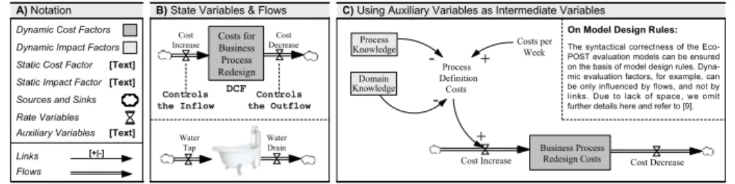
To better understand the evolution of DCF as well as DCF interference through ImF, we use economic-driven evaluation models. In particular, each DCF is represented and analyzed by exactly one evaluation model. These models are specified using the System Dynamics [11, 12] notation (cf. Fig. 1A) [7].

Model Notation. An evaluation model comprises a set of model variables which are denoted as evaluation factors. In our context SCF, DCF, and ImF correspond to evaluation factors. Different types of variables exist. State variables can be used to represent dynamic factors, i.e., to capture changing values of DCF (e.g., the ”Costs for Business Process Redesign”; cf. Fig. 1B) and dynamic ImF (e.g., a certain degree of

”Process Knowledge”). A state variable is graphically denoted as rectangle (cf. Fig. 1B), and its value at time t is determined by the accumulated changes of this variable from starting point t₀to present moment t (t>t₀); similar to a bathtub which accumulates - at a defined moment t - the amount of water which has been poured into it in the past.

Each state variable needs to be connected to at least one source or sink. Both sources and sinks are graphically denoted as cloud-like symbols (cf. Fig. 1B).

B) State Variables & Flows

Costs for Business Process Redesign

Controls the Inflow

Controls the Outflow DCF Cost Increase

Cost Decrease A) Notation

Flows Auxiliary Variables Rate Variables Dynamic Cost Factors

Links Sources and Sinks Dynamic Impact Factors

[Text]

[+|-]

Static Cost Factor [Text]

Static Impact Factor [Text]

C) Using Auxiliary Variables as Intermediate Variables

Business Process Redesign Costs

Cost Increase Cost Decrease

Process Definition

Costs Process

Knowledge

Domain Knowledge

- -

+

Costs per

+ Week

Water Tap

Water Drain

On Model Design Rules:

The syntactical correctness of the Eco- POST evaluation models can be ensured on the basis of model design rules. Dyna- mic evaluation factors, for example, can be only influenced by flows, and not by links. Due to lack of space, we omit further details here and refer to [9].

Fig. 1. Evaluation Model Notation, Mapping Rules, and initial Examples.

Values of state variables change through inflows and outflows. Graphically, both flow types are depicted by twin-arrows which either point to (in the case of an inflow) or out of (in the case of an outflow) the state variable (cf. Fig. 1B). Picking up again the bathtub image, an inflow is a pipe that adds water to the bathtub, i.e., inflows increase the value of a state variable. An outflow, by contrast, is a pipe that purges water from the bathtub, i.e., outflows decrease the value of a state variable. The DCF ”Costs for

(4)

Business Process Redesign” shown in Fig. 1C, for example, increases through its inflow (”Cost Increase”) and decreases through its outflow (”Cost Decrease”). Returning to the bathtub image, we further need ”water taps” to control the amount of water flowing into the bathtub, and ”drains” to specify the amount of water flowing out. For this purpose, a rate variable is assigned to each flow (graphically depicted by a valve; cf. Fig. 1B).

Besides state variables, evaluation models may comprise constants and auxiliary variables (which are both graphically represented by their name). Constants are used to represent static evaluation factors, i.e., SCF and static ImF in our context. Auxiliary variables, in turn, represent intermediate variables. As an example consider the auxiliary variable ”Process Definition Costs” in Fig. 1C. Both are integrated into an evaluation model with links (not flows), i.e., with labeled arrows. A positive link (labeled with a

”+”) between x and y (with y as dependent variable) indicates that y will tend in the same direction if a change occurs in x. A negative link (labeled with a ”-”) denotes that the dependent variable y will tend in the opposite direction if the value of x changes.

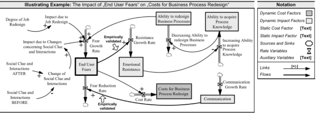
Illustrating Example. Fig. 2 shows a model which describes the influence of the dynamic ImF ”End User Fears” on the DCF ”Costs for Business Process Redesign”.

More specifically, this model reflects the assumption that the introduction of a PAIS may cause end user fears, e.g., due to a high degree of job redesign and due to changed social clues. Such end user fears can lead to emotional user resistance. This, in turn, results in a decreasing ability to acquire process knowledge. Reason is that an increasing emotional resistance makes profound process analysis (e.g., based on interviews with process participants) a difficult task to accomplish. A decreasing ability to acquire process knowledge results in a decreasing ability to redesign business processes.

Notation Illustrating Example: The Impact of „End User Fears“ on „Costs for Business Process Redesign“

Links Sources and Sinks

End User Fears

Emotional Resistance Fear

Growth Rate

Resistance Growth Rate

Ability to redesign Business Processes Degree of Job

Redesign

Social Clue and Interactions

BEFORE

Impact due to Job Redesign

Impact due to Changes concerning Social Clue and Interactions

+

+ +

AFTER Change of

+ +

+

Decreasing Ability to redesign Business

Processes

+

Communication Communication

Growth Rate Fear Reduction

Rate

+

Ability to acquire Process Knowledge

Increasing Ability to acquire Process Knowledge

- +

Costs for Business Process Redesign Cost Rate

+

Dynamic Impact Factors

[Text]

[+|-]

Empirically validated

-

Static Impact Factor [Text]

Fig. 2. Dealing with the Impact of End User Fears.

To empirically confirm our assumptions as represented in this (and other) evaluation models we conduct empirical and experimental research activities (see [13, 14]).

3 Simulating EcoPOST Evaluation Models

Evaluation models like the one depicted in Fig. 2 are of significant value for PAIS engineers. However, the evolution of DCF and dynamic ImF is difficult to comprehend.

(5)

For this reason, we added components for analyzing these dynamic implications to our overall evaluation framework. More precisely, this section describes how evaluation models can be simulated in order to unfold their dynamic effects. Section 3.1 explains why simulation is needed in our context. Section 3.2 illustrates the general computation of a simulation. Based on this, Section 3.3 deals with the specification of simulation models. Section 3.4 gives an illustrating example.

3.1 Feedback Loops

The change of DCF and dynamic ImF is caused by the interplay of the different elements of an evaluation model, i.e., the complex interdependencies between dynamic and static evaluation factors, flows and links. In this context, feedback loops are of particular importance.

Feedback Loops. A feedback loop is a closed cycle of causes and effects. Within this cycle, past events (like the change of a DCF or dynamic ImF) are utilized to control future actions (like another change of the same evaluation factor). In other words, if a change occurs in a model variable which is part of a feedback loop, this change will be propagated around the loop [12].

As an example consider the feedback loop depicted in Fig. 2. Basic to this model is a cyclic structure connecting the four dynamic ImF ”End User Fears”, ”Emotional Resistance”, ”Ability to acquire Process Knowledge”, and ”Ability to redesign Business Processes”. As aforementioned, it reflects the assumption that the introduction of a PAIS may cause end user fears, e.g., due to a high degree of job redesign. Such end user fears lead to increased emotional resistance. Increased resistance decreases the ability to get support from end users during process redesign. This, in turn, decreases the ability to effectively redesign business processes. Finally, a lower ability to redesign business processes results in decreased end user fears. Reason is that the end users will be less afraid of change if the ability to redesign processes decreases.

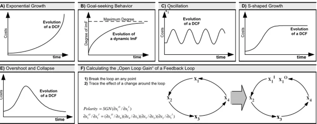
We distinguish between two types of loop polarities. First, positive (or self-rein- forcing) loops generate growth of DCF and dynamic ImF (cf. Fig. 3A). Second, nega- tive (or self-correcting) loops counteract and oppose growth (cf. Fig. 3B). If evaluation models contain both positive and negative feedback loops, more complex effects may emerge (cf. Fig. 3 C-E).

The polarity of a feedback loop is equivalent to the sign of the open loop gain.

”Gain” refers to the strength of the change returned by a loop and ”open loop” means that the gain is calculated for just one feedback cycle by opening the closed loop at some point [15]. Consider Fig. 3F which shows a closed feedback loop consisting of four variables x₁, ...,x₄. Assume that we open the loop at x₁(though any other variable of the loop can be used as well). Opening the loop at x₁splits this variable into an input variable (xÎ₁) and an output variable (x₁Ô). The open loop gain is then defined as the (partial) derivative of xÔ₁ with respect to xÎ₁, that is, the feedback effect of a change in a variable as it is propagated around a loop. Thus, the polarity of loop can be calculated as SGN(δxÔ₁/δxÎ₁), whereSGN() is the sign function, returning +1 if the argument is positive, and -1 otherwise (if the open loop gain is zero, there is no loop).

(6)

A) Exponential Growth B) Goal-seeking Behavior C) Oscillation D) S-shaped Growth

E) Overshoot and Collapse Evolution

of a DCF

time

Costs

Evolution of a dynamic ImF

time Maximum Degree

Degree of ImF Costs

time Evolution of a DCF

Costs

time Evolution

of a DCF

Costs

time Evolution of a DCF

F) Calculating the „Open Loop Gain“ of a Feedback Loop 1) Break the loop an any point

2) Trace the effect of a change around the loop x1

I

x1

x2

x₃ x4

x1 I

x2

x3

x4

x₁^O

) / )(

/ )(

/ ( /

) / (

1 2 2 3 3 4 4 1 1 1

1 1

I O

x x x x x x x x x x

x x SGN Polarity

∂

=

∂

=

Fig. 3. Feedback in Evaluation Models: Overview of potential dynamic Effects.

It is important to mention that all dynamic effects caused by feedback loops are typically not easily understandable [16]. For this reason, we investigate the effects of feedback loops through simulation¹of respective evaluation models.

3.2 Computing a Simulation

In the EcoPOST framework, simulation is based on the step-by-step numerical solution of algebraic equations specifying how to start a simulation from an existing start con- dition and how to compute succeeding conditions. In other words, the equations define how the variables of an evaluation model change over time [17].

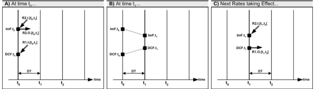
Illustrating Example. Consider Fig. 4 which depicts the simulation of two dynamic evaluation factors: a DCF and a dynamic ImF. The condition at time t₀has been calcu- lated and the condition at time t₁is now being evaluated. DT stands for ”Difference in Time” and denotes the length of the time interval between two conditions.

DCF.t0and ImF.t0designate the two values of DCF and ImF at time t₀(cf. Fig.

4A). R1.I.[t0,t₁[is a rate variable specifying the inflow of DCF within the time inter- val[t0,t₁[. Similarly, the rate variables R2.I.[t0,t₁[and R2.O.[t0,t1[specify the inflow respectively outflow of ImF within the time interval[t0,t₁[. Therewith, all information needed to compute the new values of DCF and ImF is available.

Within the time interval[t0,t1[, the rate variables act on DCF and ImF and cause them to change. The new values of DCF and ImF at time t₁are calculated by adding and subtracting the changes represented by these rates (cf. Fig. 4B). Thereby, the sequence of computation does not matter because both DCF and ImF depend only on their own previous values and on the rates taking effect within the time interval[t0,t1[. Similarly, the order in which the rates are computed does not matter because the rates do not

1For simple evaluation models, it is sometimes possible to analytically solve the simulation model’s equations. In doing so, it becomes possible to determine a model condition in terms of any future time, not just in terms of the short time intervals between successive computations during a simulation. One would be able to substitute any particular value of future time and evaluate the future model condition without first proceeding through the intervening conditions. How- ever, analytical solutions are only possible for the minority of our evaluation models. Most evaluation models comprise nonlinear relationships making the calculation of an analytical solution impossible. For such evaluation models, only the simulation process based on a step-by-step numerical solution is available.

(7)

depend on each other. Finishing the computation creates the situation shown in Fig. 4B.

In the following, only these values are needed to compute the forthcoming rates for the [t1,t2[interval (cf. Fig. 4C).

A) At time t₀...

time t₀

ImF.t0

B) At time t₁...

time

C) Next Rates taking Effect...

time ImF.t1

DCF.t1

DT DT DT

DCF.t₀

ImF.t0

DCF.t₀

ImF.t1

DCF.t1 R1.I.[t0,t1[

R2.O.[t0,t1[ R2.I.[t0,t1[

t₁ t₂ t₀ t₁ t₂ t₀ t₁ t₂

R1.O.[t₁,t₂[ R2.I.[t1,t2[

Fig. 4. Computing a Simulation Model.

Behavioral Experiments. Note that the numerical solution of equations does not allow to directly ”jump” to some future condition without first computing through all previous conditions, i.e., there exists no general solution (describing all possible effects) which can be found based on a step-by-step numerical solution. Instead, one step-by- step numerical solution gives one time history of an evaluation model’s variables based on given parameters and initial conditions. For deriving additional information, another full step-by-step computation has to be conducted based on different conditions. There- with, it becomes possible to conduct behavioral ”experiments” based on a series of simulation runs. During these simulation runs equations are manipulated in a controlled manner to systematically investigate the effects of changed simulation parameters.

3.3 Specifying a Simulation Model

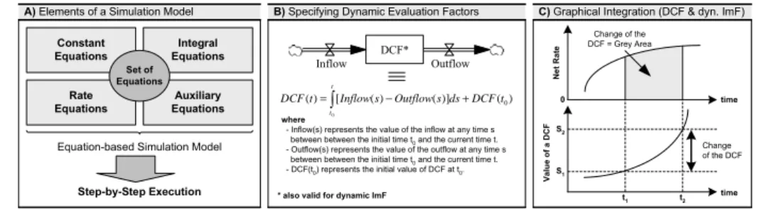
In the EcoPOST framework, a simulation model consists of a number of algebraic equa- tions - one for each model variable (i.e., dynamic and static evaluation factors as well as rate variables and auxiliary variables). The basic components of these algebraic equations are the model variables. However, we use different types of algebraic equations for the different variables of an evaluation model (cf. Fig. 5A):

– Static Evaluation Factors: Static evaluation factors (i.e., SCF and static ImF) are specified using a numerical value in a constant equation (e.g., ”Business Process Redesign Costs = 1000 $/Week”). A specific variant of a constant equation is an initially computed constant. In fact, it will often become necessary to specify a constant in terms of another constant if the former depends on the latter and the former should change in any simulation run where the latter is given a new value.

As an example of an initially computed constant consider the following equation:

Process Redesign Costs = 1000 $/Week * Risk Factor. Note that initially computed constants need to be evaluated only once at the beginning of a simulation.

(8)

– Dynamic Evaluation Factors: Dynamic evaluation factors (i.e., DCF and dynamic ImF) are specified by integral equations in our approach [16]. Such equations spec- ify the accumulation of a dynamic evaluation factor from a starting point t0to the present moment t (cf. Fig. 5B). More specifically, DCF and dynamic ImF integrate their net flow. The net flow during any interval [t₁,t₂] is the area bounded by the graph of the net rate between the start and the end of the interval (cf. Fig. 5C).

Thus, the value of a dynamic evaluation factor at t₂can be calculated as the sum of its value at t₁and the area under the net rate curve between t₁and t₂. In Fig. 5C, the value at t₁is S₁. Adding the area under the net rate curve between t₁and t₂increases the value to S₂. The net flow is determined by one or several rate variables.

B) Specifying Dynamic Evaluation Factors A) Elements of a Simulation Model

DCF*

Inflow Outflow

∫ ⁻ ⁺

=^t

t

t DCF ds s Outflow s Inflow t DCF

0

) ( )]

( ) ( [ )

( ₀

where

- Inflow(s) represents the value of the inflow at any time s between between the initial time t₀ and the current time t.

- Outflow(s) represents the value of the outflow at any time s between between the initial time t₀ and the current time t.

- DCF(t₀) represents the initial value of DCF at t₀.

C) Graphical Integration (DCF & dyn. ImF)

Change of the DCF = Grey Area

Change of the DCF S2

S₁

t1 t

2

Net RateValue of a DCF

0

time time Constant

Equations

Integral Equations

Rate Equations

Auxiliary Equations

Equation-based Simulation Model

Step-by-Step Execution * also valid for dynamic ImF Set of

Equations

Fig. 5. Integration of Flows for Dynamic Evaluation Factors.

– Rate Variables: Rate variables are expressed by rate equations. Rate equations specify the change of dynamic evaluation factors (DCF or dynamic ImF) between two computed conditions (cf. Section 3.2). More specifically, rate equations for flows connected to DCF specify the amount of costs flowing to, from, or between DCF. Rate equations for flows connected to dynamic ImF specify the impact flowing to, from, or between dynamic ImF. In any case, a rate equation uses information (i.e., values) from other model variables (SCF, DCF, dynamic ImF, and auxiliary variables) to calculate a specific change. In the context of a specific rate variable, the relevant information is represented by those model variables that are connected to the rate variable by links (cf. Section 2.2).

– Auxiliary Variables: Auxiliary variables are specified by auxiliary equations. Their constituting elements may be SCF, DCF, dynamic ImF, rate variables, and auxiliary variables. Auxiliary equations are evaluated after the integral equations on which they depend, and before the rate equations of which they are part.

The total set of equations of a given evaluation model is denoted as simulation model.

For the design of our evaluation models as well as their simulation we have used the visual modeling and simulation tool Vensim [18].

3.4 Specifying nonlinear Relationships through Table Functions

An important part of our evaluation models are ImF (e.g., process knowledge, domain knowledge, end user fears). Often, an ImF has a nonlinear impact on DCF. Such non-

(9)

linearities have to be represented in our simulation models as well. For this purpose, we use a specific kind of auxiliary equation (implying that nonlinearities require the introduction of additional auxiliary variables in our evaluation models). Specifically, we use table functions transferring an input value (e.g., a certain degree of process knowledge) into a corresponding output value (e.g., expressing a specific effect on a DCF). More specifically, we can define (with Y representing an ImF and X representing a DCF):

Definition A function Y=f(X)is called table function, if it is represented as follows:

– Y = Effect of X on Y,

– Effect of X on Y = Table for Effect of X on Y(X), – Table for Effect of X on Y =(x1,y₁),(x2,y₂), ...,(xn,y_n),

where(xi,yi)represents each pair of points defining the relationship.

In other words, the output value Y is calculated dependent on the input value X through lookup function f . Linear interpolation is used for values lying between the specified table values. Fig. 6 illustrates the specification of table functions in Vensim [18], the visual modeling and simulation tool we use.

Fig. 6. Specifying Table Functions (left) and Table of Values (right) in Vensim [18].

Fig. 7 shows typical table functions. Dependent on the degree of an ImF (represented by X ) a specific impact rating is derived (represented by Y ). An impact rating less than 1 results in decreasing costs (cf. Fig. 7A). A rating equal to 1 neither does increase nor decrease costs. A rating larger than 1 results in increasing costs (cf. Fig. 7B and Fig.

7C). Quantifications based on such impact ratings are also known from software cost models like COCOMO [19].

The information needed for specifying the shape and the values of table functions can be derived from different sources, including, for example, statistical studies, prac- tical fieldwork, and interviews. Generally, there exists no standard way of building ro- bust table functions though a ”best practice” guideline for formulating table functions is given in [15] (cf. Fig. 8). It is important to mention that the input and output values of table functions are typically normalized. This means that the input value is a dimension- less ratio of the input to a reference value X^∗and the output value is a dimensionless effect modifying the reference value Y^∗, i.e., Y=Y^∗f(X/X^∗).

(10)

0 0 1

1

Impact Due to Impact Factor

Degree of Impact Factor (normalized)

IR = f(x) with x, IRin [0,1]

Impact

Impact Rating (IR) < 1

0 1 2

1

Impact on DCF due to Impact Factor

Degree of Impact Factor (normalized) 0 1 2

1

Impact on DCF due to Impact Factor

Degree of Impact Factor (normalized)

IR = f(x) with x in [0,1] and IR in [1,2] IR = f(x) with x in [0,1] and IR in [1,2]

Impact Impact

Impact Rating (IR) > 1

A B C

Fig. 7. Table Functions for quantifying Impact Factors.

Normalize the input and output.

Normalize the table function so that the input is the dimensionless ratio of the input to a reference value X* and the output is a dimensionless effect modifying the reference value Y*, i.e., Y=Y*f(X/X*).

Identify reference points. Indentify the reference points where the values of the function are determined by definition. In normalized functions, the function usually must pass through the point (1,1) so that Y=Y* when X=X*.

Identify reference policies.

Reference policies are lines or curves corresponding to standard or extreme policies. The reference policy f(X/X*)=1, for example, represents the policy that X has no effect on Y. The 45° line represents the policy that Y varies 1% for every 1% change in X and is often a meaningful reference policy.

Consider extreme conditions.

What values must the function take at extremes? If there are multiple nonlinear effects in the formulation, check that the formulation makes sense for all combinations of extreme values and that the slopes of the effects at the normal operating points conform to any reference policies and constraints on the overall response of the output.

Specify the domain for the independent variable.

Specify the domain for the independent variable so that it includes the full range of possible values, including extreme conditions, not only the normal operating region.

Identify the plausible shapes for the function.

Identify the plausible shapes for the function within the feasible region defined by the extreme conditions, refeence points, and reference policy lines. Select the shape you believe best corresponds to the data (numerical and qualitative). Justify any inflection points. Interpret the shapes in terms of the physical constraints and policies of the decision maker.

Specify the values for your best estimate

of the function.

Use increments small enough to get the smoothness you require. Examine the increments between values to make sure there are no kinks you cannot justify. If numerical data are available you can often estimate the values statistically. Otherwise, make a judgmental estimate using the best information. Often, judgmental estimates provide sufficient accuracy, particularly early in a project, and help focus subsequent modeling and data collection efforts.

Run and test the model

Run the model and test to make sure the behavior of the formulation and nonlinear function is reasonable. Check that the input varies over the appropriate range (e.g., that the inputs is not operating off the ends of the function at all times).

Test the sensitivity of your results.

Test the sensitivity of your results to plausible variations in the values of the function. If sensitivity analysis shows that the results change significantly over the range of uncertainty in the relationship, you need to gather more data to reduce the uncertainty. If the results are not sensitive to the assumed values, then you do not need to spend additional resources to estimate the function more accurately.

1

9 8 7 6 5 4 3 2

Fig. 8. Guideline for building Table Functions [15].

(11)

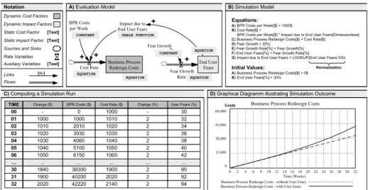
3.5 Illustrating Example

Fig. 9A shows a simple evaluation model. Assume that the evolution of the DCF ”Costs for Business Process Redesign” (caused by the dynamic ImF ”End User Fears”) shall be analyzed (ignoring other potential ImF). The model reflects the assumption that the redesign of business processes (e.g., prior to the introduction of a PAIS) may be influenced by end user fears (caused by a high degree of job redesign or changed social clues). Such end user fears can lead to emotional resistance of users, and, in turn, to a lack of support from the users while redesigning business processes, e.g., during an interview-based process analysis.

A) Evaluation Model

C) Computing a Simulation Run

TIME Change ($) BPR Costs ($)

00 - 0

01 1000 1000

02 1010 2010

03 1020 3030

04 1030 4060

05 1040 5100

06 1050 6150

... ... ...

30 1840 38300

31 1900 40200

32 2020 42220

Notation

Links Sources and Sinks Dynamic Impact Factors

[Text]

[+|-]

Static Impact Factor[Text]

TABLE FUNCTION

EQUATION

Business Process Redesign Costs 60,000

45,000

30,000

15,000

0

0 2 4 6 8 101214161820 22 24 26 28 3032

Time (Weeks) Business Process Redesign Costs : without User Fears Business Process

Redesign Costs

End User Fears Fear Growth

Rate Cost Rate

Impact due to End User Fears BPR Costs

per Week

Fear Growth

B) Simulation Model Equations:

A) BPR Costs per Week[$] = 1000$

B) Cost Rate[$] =

BPR Costs per Week[$] * Impact due to End User Fears[Dimensionless]

C) Business Process Redesign Costs[$] = Cost Rate[$]

D) Fear Growth = 2[%]

E) Fear Growth Rate[%] = Fear Growth[%]

F) End User Fears[%] = Fear Growth Rate[%]

G) Impact due to End User Fears = LOOKUP(End User Fears/100) Initial Values:

A) Business Process Redesign Costs[$] = 0$

B) End User Fears[%] = 30%

Cost Rate ($) 1000 1010 1020 1030 1040 1050 1060 ...

1900 2020 2140

Change (%) - 2 2 2 2 2 2 ...

2 2 2

User Fears (%) 30 32 34 36 38 40 42 ...

90 92 94

D) Graphical Diagramm illustrating Simulation Outcome

Business Process Redesign Costs : with User Fears Costs

CONSTANT

CONSTANT EQUATION

EQUATION EQUATION

Normalization

+ +

Fig. 9. Dealing with the Impact of End User Fears.

Assume that the business process redesign activities are scheduled for 32 weeks. In order to simulate the evolution of the resulting costs along this time frame, we use the simulation model depicted in Fig. 9B. Here, the nonlinear impact of end user fears on the costs of business process redesign is represented through a table function. Fig. 9C shows the values of the evaluation model’s dynamic evaluation factors over time when the simulation model is executed. The underlying principles of this computation have been already described in Section 3.2. Finally, Fig. 9D shows a graphical diagram which illustrates the outcome of the simulation. As can be seen, there is a significant negative impact of end user fears on the costs of business process redesign.

4 Related Work

Basically, one can distinguish between six major categories of cost estimation tech- niques [20]: model-based approaches (e.g., COCOMO, SLIM), expertise-based ap- proaches (e.g., the Delphi method), learning-oriented approaches (using neural net- works or case based reasoning), regression-based approaches (e.g., the ordinary least

(12)

squares method), composite approaches (e.g., the Bayesian approach), and dynamic- based approaches (which explicitly acknowledge that cost factors change over the du- ration of the system development). Picking up this classification, our framework can be considered as an example of a dynamic-based approach (the other five categories rely on static analysis models). Besides, IT evaluation approaches have to be considered as well. Due to lack of space, we omit further details here and refer to [7].

Recently, equation-based simulation approaches (as envisioned in our EcoPOST framework) often compete with agent-based simulation. Agent-based simulations are based on a set of agents (e.g., reactive agents, intentional agents, social agents) encap- sulating the behavior of the various variables that make up a system [21]. During a simulation, the behavior of these agents is emulated. Generally, agent-based simulation is less quantitative and more qualitative than equation-based simulation. Invariants do not come in the form of equations, but in the form of rules, and this makes agent-based simulation an interesting alternative, particularly in purely social environments, but also in environments that include both social and technological variables. When compared to equation-based approaches, agent-based approaches do not begin with specifying equations that relate observed variables to one another, but with behaviors through which individuals interact [22]. Thereby, agent-based approaches define agent behavior in terms of variables accessible to individual agents. This leads away from reliance on system-level information as extensively done by equation-based approaches (since it is often easier to formulate parsimonious closed-form equations using such quantities).

However, as equation-based simulation is easier to use in practice (which is one major requirement guiding the development of the EcoPOST framework), we have not considered the use of agent-based simulation.

5 Summary

The EcoPOST framework enables PAIS engineers to model the complex interplay between the numerous cost and impact factors which arise in the context of PAIS engineering projects. Fig. 10 depicts the main pillars of the EcoPOST framework [10]. This paper has focused on the use of simulation to investigate the dynamic effects described by our evaluation models (particularly the evolution of DCF).

Empirical &

Experimental Research Economic-driven

Evaluation Models Simulation Value-based Evaluation Patterns

Governance Guidelines

EcoPOST Cost Benefit Analyzer

I II III IV V VI

Fig. 10. Main Components of the EcoPOST Framework.

In particular, our paper has illustrated the use of simulation to investigate the dynamic implications described by EcoPOST evaluation models. We have motivated the use of computer simulation as a means to analyze the dynamic effects caused by feedback loops. We have described the constituting elements of EcoPOST simulation models and

(13)

have discussed the execution of simulation models. Finally, we have given an example illustrating the basic notion of simulating dynamic evaluation factors.

Note that the expressiveness of simulation always depends on the plausibility and resilience of the underlying simulation models. Therefore, we have additionally accomplished various empirical and experimental research activities (e.g., software experiments, online surveys, case studies) in order to put the quantifications gained from our simulation models on a more reliable basis (see [13] for examples).

References

1. Reichert, M., Rinderle, S., Kreher, U., Dadam, P.: Adaptive Process Management with ADEPT2. Proc. 21th ICDE ’05, pp.1113-1114 (2005)

2. Dumas, M., van der Aalst, W.M.P., ter Hofstede, A.H.: Process-aware Information Systems:

Bridging People and Software through Process Technology. Wiley (2005)

3. Reijers, H.A., van der Aalst, W.M.P.: The Effectiveness of Workflow Management Systems - Predictions and Lessons Learned. Int’l. J. of Inf. Manag., 25(5), pp.457-471 (2005) 4. Choenni, S., Bakkera, R., Baetsa, W.: On the Evaluation of Workflow Systems in Business

Processes. Electronic Journal of IS Evaluation (EJISE), 6(2) (2003)

5. Oba, M., Onoda, S., Komoda, N.: Evaluating the Quantitative Effects of Workflow Systems based on Real Cases. Proc. 33rd HICSS (2000)

6. Kleiner, N.: Can Business Process Changes Be Cheaper Implemented with Workflow- Management-Systems? Proc. IRMA ’04, pp.529-532 (2004)

7. Mutschler, B., Reichert, M., Bumiller, J.: Designing an Economic-driven Evaluation Frame- work for Process-oriented Software Technologies. Proc. 28th ICSE, pp.885-888 (2006) 8. Yu, E.: Modelling Strategic Relationships for Process Reengineering. PhD Thesis, University

of Toronto (1995)

9. Mutschler, B., Reichert, M., Bumiller, J.: An Approach for Evaluating Workflow Manage- ment Systems from a Value-Based Perspective. Proc. 10th IEEE EDOC, pp.477-482 (2006) 10. Mutschler, B., Reichert, M.: Analyzing the Dynamic Cost Factors of Process-aware Infor-

mation Systems: A Model-based Approach. Proc. CAiSE ’07 (to appear) (2007) 11. Richardson, G.P., Pugh, A.L.: System Dynamics - Modeling with DYNAMO. (1981) 12. Ogata, K.: System Dynamics. Prentice Hall (2003)

13. Mutschler, B., Reichert, M., Bumiller, J.: Why Process-Orientation is Scarce: An Emp. Study of Process-oriented IS in the Autom. Industry. Proc. 10th IEEE EDOC, pp.433-438 (2006) 14. Mutschler, B., Reichert, M.: A Survey on Evaluation Factors for Business Process Manage-

ment Technology. Technical Report, TR-CTIT-06-63, University of Twente (2006) 15. Sterman, J.D.: Business Dynamics - Systems Thinking and Modeling. McGraw-Hill (2000) 16. Forrester, J.W.: Industrial Dynamics. Productivity Press, Cambridge, London (1961) 17. Vangheluwe, H., de Lara, J., Mosterman, P.J.: An Introduction to Multi-Paradigm and Sim-

ulation. Proc. AIS ’02, pp.9-20 (2002)

18. Vensim: Ventana Systems. http://www.vensim.com/ (2006)

19. Boehm, B., Abts, C., Brown, A.W., Chulani, S., Clark, B.K., Horowitz, E., Madachy, R., Reifer, D., Steece, B.: Software Cost Estimation with Cocomo 2. Prentice Hall (2000) 20. Boehm, B., Abts, C., Chulani, S.: Software Development Cost Estimation Approaches - A

Survey. Technical Report, USC-CSE-2000-505 (2000)

21. Brassel, K.H., Mhring, M., Schumacher, E., Troitzsch, K.G.: Can Agents Cover All the World? Simulating Social Phenomena, LNEMS 456, Springer (1997)

22. Scholl, H.J.: Agent-based and System Dynamics Modeling: A Call for Cross Study and Joint Research. Proc. 34th Int’l. Conf. on System Sciences (2001)