Exploring the Dynamic Costs of Process-aware Information Systems through Simulation
Bela Mutschler and Manfred Reichert
Information Systems Group, University of Twente, The Netherlands {b.b.mutschler;m.u.reichert}@utwente.nl
Abstract. Introducing process-aware information systems (PAIS) in enterprises (e.g., workflow management systems, case handling systems) is associated with high costs. Though cost evaluation has received considerable attention in software engineering for many years, it is difficult to apply existing evaluation approaches to PAIS. This difficulty particularly stems from the inability of these techniques to deal with the complex interplay of the many technological, organizational and project-driven factors which emerge in the context of PAIS engineering projects.
In response to this problem this paper proposes an approach which utilizes si- mulation models for investigating costs related to PAIS engineering projects. We motivate the need for simulation, discuss the design and execution of simulation models, and give an illustrating example.
Keywords: Cost Modeling, Simulation Models, Method Engineering.
1 Introduction
Process-aware information systems (PAIS) separate process logic from application code and orchestrate business processes according to their defined logic during run-time [1]. To enable the realization of PAIS, a variety of process support paradigms (e.g., workflow management, service flows, case handling), process modeling standards (e.g., BPEL4WS, BPML), and process management tools (e.g., ARIS Toolset, Staffware) have been introduced [2].
While the benefits of PAIS are typically justified by improved business process per- formance [3–5] and cheaper process implementation [6], there exist no approaches for systematically analyzing related costs. In particular, existing cost evaluation techniques are unable to cope with the numerous technological, organizational and project-driven factors to be considered in the context of a PAIS (and which do only partly exist in projects developing data- or function-centered information systems) [7]. As an exam- ple, consider costs for analyzing and redesigning business processes. Another challenge results from the many causal dependencies between evaluation factors. Activities re- lated to business process redesign, for example, can be influenced by impact factors like available process knowledge or end user fears. These dependencies result in dynamic economic effects which can influence the overall costs of a PAIS engineering project significantly. Existing approaches are typically not able to deal with such effects as they rely on static models based upon snapshots of the analyzed software system.
What is needed is a comprehensive approach that enables system engineers to model the complex interplay between the cost and impact factors that arise in the context of PAIS, and to investigate resulting effects. In response to this need we have introduced the notion of evaluation models in [8, 9]. This paper deals with the simulation of the dy- namic costs of PAIS engineering projects. Section 2 describes background information necessary for understanding the paper. Section 3 deals with simulation as envisioned in our approach. Section 4 concludes with a summary.
2 The EcoPOST Evaluation Framework
In [8, 9] we have introduced a model-based approach for systematically investigating the complex cost structures of PAIS engineering projects. This approach distinguishes between different kinds of evaluation factors to be considered when dealing with the costs of PAIS engineering projects.
Terminology. A Static Cost Factors (SCF) represent costs whose value does not change during a PAIS engineering project (except for its time value, which is not fur- ther considered in this paper). As typical examples of SCF consider software license costs, hardware costs, or costs for external consultants. Dynamic Cost Factors (DCF), in turn, represent costs that are determined by activities related to a PAIS engineering project. These activities cause measurable efforts, which, in turn, vary due to the influ- ence of impact factors. The (re)design of business processes prior to the introduction of PAIS, for example, constitutes such an activity. The DCF ”Costs for Business Process Redesign”, for instance, may be influenced by an intangible factor ”Willingness of Staff Members to support Redesign Activities”. Obviously, if staff members do not contribute to a redesign project by providing needed information (e.g., about process details), any redesign effort will be ineffective and will increase costs. If staff willingness is addi- tionally varying during the redesign activity (e.g., due to a changing communication policy), the DCF will be subject to more complex effects.
In the EcoPOST framework, intangible factors like ”Willingness of Staff Members to support Redesign Activities” are represented by Impact Factors (ImF). They are in- tangible evaluation factors that influence DCF (or more precisely, the activities under- lying a DCF). ImF cause the value of a DCF to change, making the evaluation of DCF a difficult task to accomplish. As examples consider factors such as ”End User Fears”,
”Availability of Process Knowledge”, or ”Ability to redesign Business Processes”. Op- posed to SCF and DCF, the values of ImF are not quantified in monetary terms, but are based on qualitative scales describing the degree of an ImF (ranging from ”low” to
”high”). ImF can be further classified into static and dynamic ImF. The value of a static ImF does not change. The value of a dynamic ImF, by contrast, may change (due to the influence of other ImF).
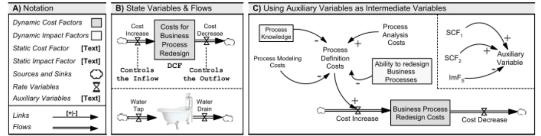
Evaluation Models. To better understand the evolution of DCF as well as DCF interference through ImF, we use evaluation models. In particular, each DCF is repre- sented and analyzed by exactly one evaluation model. These models are specified using the System Dynamics (SD) [10–12] notation (cf. Fig. 1A) [13]. SCF, DCF, and ImF are represented by different types of variables. State variables, for example, are used to represent dynamic factors, i.e., to capture changing values of DCF (e.g., the ”Costs for
Business Process Redesign”; cf. Fig. 1B) and dynamic ImF (e.g., degree of ”Process Knowledge”). A state variable is graphically denoted as rectangle (cf. Fig. 1B), and its value at time t is determined by the accumulated changes of this variable from starting point t0 to present moment t (t>t0); similar to a bathtub which accumulates – at a defined moment t – the amount of water which has been poured into it in the past. Each state variable needs to be connected to at least one source or sink. Both sources and sinks are graphically denoted as cloud-like symbols.
B) State Variables & Flows
Costs for Business Process Redesign
Controls the Inflow
Controls the Outflow DCF Cost Increase
Cost Decrease A) Notation
Flows Auxiliary Variables Rate Variables Dynamic Cost Factors
Links Sources and Sinks Dynamic Impact Factors
[Text]
[+|-]
Static Cost Factor [Text]
Static Impact Factor [Text]
C) Using Auxiliary Variables as Intermediate Variables
Business Process Redesign Costs
Cost Increase Cost Decrease
Process Definition Costs Process
Knowledge
Process Modeling Costs
-
- +
Process Analysis Costs
+
Water Tap
Water Drain
SCF1
SCF2 ImFS
Auxiliary Variable
+ +
Ability to redesign -
Business Processes
-
Fig. 1. Evaluation Model Notation and initial Examples.
Values of state variables change through inflows and outflows. Graphically, both flow types are depicted by twin-arrows which either point to (in the case of an inflow) or out of (in the case of an outflow) the state variable (cf. Fig. 1B). Picking up the bathtub image, an inflow is a pipe that adds water to the bathtub, i.e., inflows increase the value of a state variable. An outflow, by contrast, is a pipe that purges water from the bath- tub, i.e., outflows decrease the value of a state variable. The DCF ”Costs for Business Process Redesign” as shown in Fig. 1C, for example, increases through its inflow ”Cost Increase” and decreases through its outflow ”Cost Decrease”. Returning to the bathtub image, we further need ”water taps” to control the amount of water flowing into the bathtub, and ”drains” to specify the amount of water flowing out. For this purpose, a rate variable is assigned to each flow (graphically depicted by a valve; cf. Fig. 1B).
In addition to state variables representing DCF and dynamic ImF, evaluation models comprise constants and auxiliary variables (which are both graphically represented by their name). Constants are used to represent static evaluation factors, i.e., SCF and static ImF in our context. As an example for a SCF consider license costs. As an example for a static ImF consider a given degree of ”Process Complexity”. Auxiliary variables, in turn, represent intermediate variables. As an example consider the auxiliary variable
”Process Definition Costs” in Fig. 1C. Both constants and auxiliary variables are em- bedded in an evaluation model with links (not flows), i.e., labeled arrows. A positive link (labeled with ”+”) between x and y (with y as dependent variable) indicates that y will tend in the same direction if a change occurs in x. A negative link (labeled with
”-”) expresses that the dependent variable y will tend in the opposite direction.
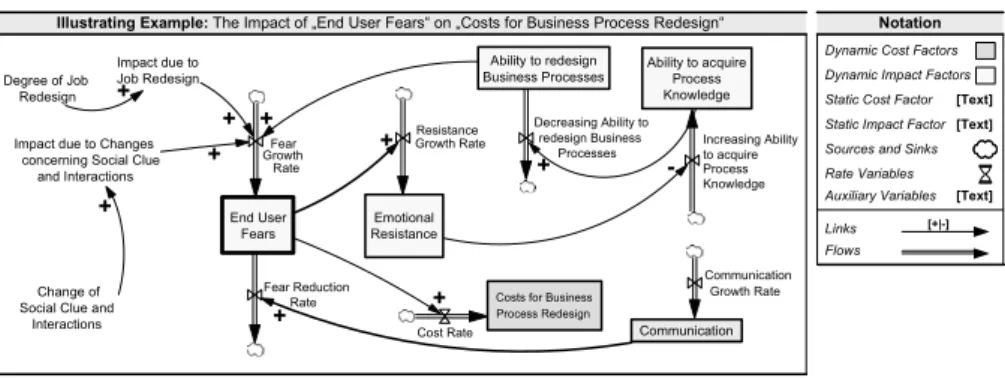
Illustrating Example. Fig. 2 shows a model which describes the influence of the dynamic ImF ”End User Fears” on the DCF ”Costs for Business Process Redesign”.
More specifically, this model reflects the assumption that the introduction of a PAIS may cause end user fears, e.g., due to a high degree of job redesign and due to changed social clues. Such end user fears can lead to emotional user resistance. This, in turn,
results in a decreasing ability to acquire process knowledge. Reason is that an increas- ing emotional resistance makes profound process analysis (e.g., based on interviews with process participants) a difficult task to accomplish. A decreasing ability to acquire process knowledge results in a decreasing ability to redesign business processes.
Notation Illustrating Example: The Impact of „End User Fears“ on „Costs for Business Process Redesign“
Flows Auxiliary Variables Rate Variables Dynamic Cost Factors
Links Sources and Sinks
End User Fears
Emotional Resistance Fear
Growth Rate
Resistance Growth Rate
Ability to redesign Business Processes Degree of Job
Redesign
Impact due to Job Redesign
Impact due to Changes concerning Social Clue
and Interactions
+
+ +
Change of Social Clue and
Interactions
+
+ Decreasing Ability to
redesign Business Processes
+
Communication Communication
Growth Rate Fear Reduction
+Rate
Ability to acquire Process Knowledge
Increasing Ability to acquire Process Knowledge
+ -
Costs for Business Process Redesign Cost Rate
+
Dynamic Impact Factors
[Text]
[+|-]
Static Cost Factor [Text]
Static Impact Factor [Text]
Fig. 2. Dealing with the Impact of End User Fears.
3 Simulating EcoPOST Evaluation Models
Evaluation models, like the one depicted in Fig. 2, are very useful for PAIS engineers.
However, the evolution of DCF and dynamic ImF is difficult to comprehend. For this reason, we add components for analyzing this evolution to our overall evaluation frame- work. More precisely, this section describes how evaluation models can be simulated in order to unfold their dynamic effects.
3.1 Understanding PAIS Engineering Projects as Feedback Systems
As mentioned, we use System Dynamics (SD) for defining evaluation models. SD is a formalism for studying and modeling complex feedback systems, as they can be found, for example, in biological, environmental, industrial, business, and social systems [10, 11]. Its underlying assumption is that human mind is excellent in observing the elemen- tary forces and actions out of which a system is composed (e.g., fears, delays, resistance to change), but unable to understand dynamic implications resulting from these forces and actions. In PAIS engineering projects we have the same situation. Such projects are characterized by a strong nexus of organizational, technological, and project-driven factors. Thereby, the identification of these factors constitutes one main problem. Far more difficult is to understand causal dependencies between factors and resulting ef- fects. Only by considering PAIS engineering projects as feedback system we are able to unfold the dynamic effects caused by these dependencies and the different organiza- tional, technological, and project-driven system parts.
”Feedback” refers to situations in which a factor X (e.g., user fears) affects another factor Y (e.g., emotional resistance of end users), and factor Y, in turn, affects X (either directly or indirectly). SD denotes such causal structures (or cyclic chains of causes and
effects) as ”feedback loops” (see below). It assumes that it is not possible to study the causal dependency between X and Y without considering the entire system.
There are other formalisms that can be used to model complex systems of interact- ing factors. Causal Bayesian Networks (BN) [14], for example, promise to be a useful approach in this context as well. BN deal with (un)certainty and focus on determin- ing probabilities of events. A BN is a directed acyclic graph which represents inde- pendencies embodied in a given joint probability distribution over a set of variables.
Variables can be measurable or intangible parameters or random variables (which form the ”Bayesian” aspect of a BN). In our context, we are interested in the interplay of the parts (components) of a system and the effects resulting from this interplay. BN do not allow to model feedback loops as cycles in BN would allow infinite feedbacks and oscillations that would prevent stable parameters of the probability distribution.
Agent-based modeling provides another promising approach. Resulting models com- prise a set of reactive, intentional, or social agents encapsulating the behavior of the various variables that make up a system [15]. During simulation, the behavior of these agents is emulated according to defined rules [16]. System-level information (e.g., about intangible factors being effective in a PAIS engineering project) is thereby not further considered. However, as system-level information is an important aspect in our ap- proach, we have not further considered the use of agent-based modeling.
3.2 Feedback Loops
Changes of DCF and dynamic ImF are caused by the interplay of the different elements of an evaluation model, i.e., the complex interdependencies between dynamic and static evaluation factors, flows and links. In this context, feedback loops are of particular im- portance. A feedback loop is a closed cycle of causes and effects. Within this cycle, past events (like the change of a DCF or dynamic ImF) are utilized to control future actions (like another change of the same evaluation factor). In other words, if a change occurs in a model variable, which is part of a feedback loop, this change will be propagated around the loop [12].
As an example consider the feedback loop depicted in Fig. 2. Basic to this model is a cyclic structure connecting the four dynamic ImF ”End User Fears”, ”Emotional Resistance”, ”Ability to acquire Process Knowledge”, and ”Ability to redesign Business Processes”. As aforementioned, it reflects the assumption that the introduction of a PAIS may cause end user fears, e.g., due to a high degree of job redesign. Such end user fears lead to increased emotional resistance. This, in turn, decreases the ability to get support from end users during process redesign and thus decreases the ability to effectively redesign business processes. Finally, a lower ability to redesign business processes results in decreased end user fears. Reason is that the end users will be less afraid of change if the ability to redesign processes decreases.
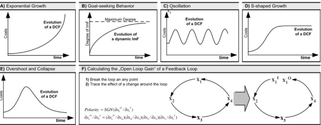
We distinguish between two kinds of loop polarities. Positive loops generate growth of DCF and dynamic ImF (cf. Fig. 3A). Negative loops, in turn, counteract and oppose growth (cf. Fig. 3B). If evaluation models contain both positive and negative feedback loops, more complex effects will result (cf. Fig. 3 C-E).
The polarity of a feedback loop is equivalent to the sign of the open loop gain.
”Gain” refers to the strength of the change returned by a loop and ”open loop” means
A) Exponential Growth B) Goal-seeking Behavior C) Oscillation D) S-shaped Growth
E) Overshoot and Collapse Evolution
of a DCF
time
Costs
Evolution of a dynamic ImF
time Maximum Degree
Degree of ImF Costs
time Evolution of a DCF
Costs
time Evolution
of a DCF
Costs
time Evolution of a DCF
F) Calculating the „Open Loop Gain“ of a Feedback Loop 1) Break the loop an any point
2) Trace the effect of a change around the loop x1
I
x1
x2
x3 x4
x1 I
x2
x3
x4
x1O
) / )(
/ )(
/ )(
/ ( /
) / (
1 2 2 3 3 4 4 1 1 1
1 1
I O
I O
I O
x x x x x x x x x x
x x SGN Polarity
∂
∂
∂
∂
∂
∂
∂
∂
=
∂
∂
∂
∂
=
Fig. 3. Feedback in Evaluation Models: Overview of potential dynamic Effects.
that the gain is calculated for just one feedback cycle by opening the closed loop at some point [12]. Consider Fig. 3F which shows a closed feedback loop consisting of four variables x1, ...,x4. Assume that we open the loop at x1. This splits x1into an input variable (xI1) and an output variable (x1O). The open loop gain is then defined as the (partial) derivative of xO1 with respect to xI1; i.e., the feedback effect of a change in a variable as it is propagated around a loop. Thus, loop polarity can be calculated as SGN(δxO1/δxI1), whereSGN()is the sign function, returning +1 in case of positive loop polarity, and -1 otherwise (if the open loop gain is zero, there will be no loop).
It is important to mention that dynamic effects caused by feedback loops are not easy to understand [11, 17]. In order to systematically investigate their effects in detail, we simulate our evaluation models.
3.3 Computing a Simulation
In the EcoPOST framework, simulation is based on a step-by-step numerical solution of algebraic equations, which specify how to perform a simulation from an initial con- dition and how to compute succeeding conditions [11]. In other words, the equations define how the variables of an evaluation model change over time.
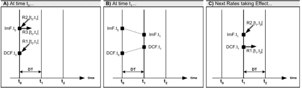
Illustrating Example. Consider Fig. 4 which depicts the simulation of two dynamic evaluation factors: a DCF and a dynamic ImF. The condition at time t0has been calcu- lated and the condition at time t1is now being evaluated. DT stands for ”Difference in Time” and denotes the length of the time interval between two conditions. DCF.t0and ImF.t0designate the two values of DCF and ImF at time t0(cf. Fig. 4A). R1.[t0,t1[is a rate variable specifying the inflow of DCF within the time interval[t0,t1[. Similarly, the rate variables R2.[t0,t1[and R3.[t0,t1[specify the inflow respectively outflow of ImF within the time interval[t0,t1[. Therewith, all information needed to compute the new values of DCF and ImF is available.
Within the time interval[t0,t1[, the rate variables act on DCF and ImF and cause them to change. The new values of DCF and ImF at time t1are calculated by adding and subtracting the changes represented by these rates (cf. Fig. 4B). Finishing the com-
A) At time t0...
t0 time ImF.t0
B) At time t1...
time
C) Next Rates taking Effect...
time ImF.t1
DCF.t1
DT DT DT
DCF.t0
ImF.t0
DCF.t0
ImF.t1 DCF.t1 R1.[t0,t1[
R3.[t0,t1[ R2.[t0,t1[
t1 t2 t0 t1 t2 t0 t1 t2
R1.[t1,t2[ R2.[t1,t2[
Fig. 4. Computing a Simulation Model.
putation creates the situation shown in Fig. 4B. In the following, only these values are needed to compute the forthcoming rates for the[t1,t2[interval (cf. Fig. 4C).
Sensitivity Analysis. Note that the numerical solution of equations does not allow to determine an arbitrary future condition during a simulation without first computing through all previous conditions. Each step-by-step numerical solution represents one simulation run with one final condition. In order to determine another condition, an ad- ditional step-by-step computation has to be conducted. Therewith, it becomes possible to conduct behavioral ”experiments” based on a series of simulation runs. During these simulation runs equations are manipulated in a controlled manner to systematically in- vestigate the effects of changed simulation parameters. Therewith, it becomes possible to accomplish sensitivity analysis, i.e., to investigate how the output of a simulation will vary if the initial condition of a simulation is changed.
3.4 Specifying a Simulation Model
In the EcoPOST framework, a simulation model consists of a number of algebraic equa- tions – one for each model variable (i.e., dynamic and static evaluation factors as well as rate variables and auxiliary variables). We use different types of algebraic equations for the different variables of an evaluation model (cf. Fig. 5A).
Elements of a Simulation Model. Static evaluation factors (i.e., SCF and static ImF) are specified based on numerical values in constant equations (e.g., ”Process Redesign Costs = 1000 $/Week”). Dynamic evaluation factors (i.e., DCF and dynamic ImF), in turn, are specified by integral equations [11]. Such equations specify the accumulation of a dynamic evaluation factor from a starting point t0to the present moment t (cf. Fig.
5B). More specifically, DCF and dynamic ImF integrate their net flow. The net flow during any interval [t1,t2] is the area bounded by the graph of the net rate between the start and the end of the interval (cf. Fig. 5C). Thus, the value of a dynamic evaluation factor at t2can be calculated as the sum of its value at t1and the area under the net rate curve between t1and t2. In Fig. 5C, the value at t1is S1. Adding the area under the net rate curve between t1and t2increases the value to S2.
Rate variables are specified by rate equations. A rate equation specifies the net change caused by a particular flow (influencing either a DCF or a dynamic ImF) be- tween two computed conditions (cf. Section 3.3). Rate equations for DCF-related flows
B) Specifying Dynamic Evaluation Factors A) Elements of a Simulation Model
DCF*
Inflow Outflow
∫ − +
=
t
t
t DCF ds s Outflow s Inflow t DCF
0
) ( )]
( ) ( [ )
( 0
where
- Inflow(s) represents the value of the inflow at any time s between between the initial time t0 and the current time t.
- Outflow(s) represents the value of the outflow at any time s between between the initial time t0 and the current time t.
- DCF(t0) represents the initial value of DCF at t0.
C) Graphical Integration (DCF & dyn. ImF) Change of the
DCF = Grey Area
Change of the DCF S2
S1
t1 t2
Net RateValue of a DCF
0
time time Constant
Equations
Integral Equations
Rate Equations
Auxiliary Equations
Equation-based Simulation Model
Step-by-Step Numerical Solution * also valid for dynamic ImF Set of
Equations
Fig. 5. Integration of Flows for Dynamic Evaluation Factors.
specify the ”amount of costs” flowing to, from, or between DCF. Rate equations for ImF-related flows specify the ”impact” flowing to, from, or between dynamic ImF. A rate equation comprises those model variables which influence the flow it controls. This can be SCF, DCF, dynamic ImF, and auxiliary variables.
Finally, auxiliary variables are specified by auxiliary equations. Their constituting elements may be static and dynamic evaluation factors as well as other auxiliary vari- ables. Though the value of auxiliary variables changes during simulation, they do not represent a model state. Instead, they are used for intermediate calculations.
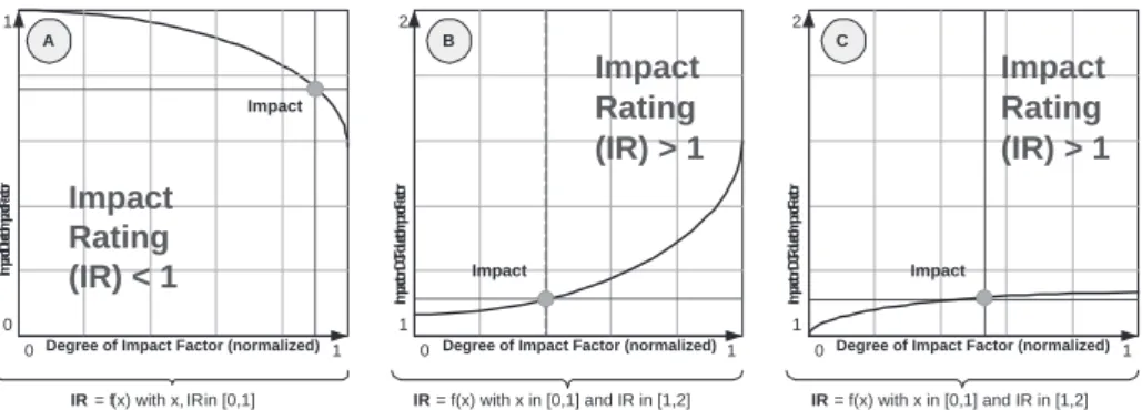
Nonlinear Relationships. An important part of our evaluation models are ImF. If an (either static or dynamic) ImF has a nonlinear impact on DCF, such nonlinearities will have to be represented in our simulation models as well. In our simulation models, nonlinearities are represented by an additional auxiliary variable between the ImF and the DCF. This auxiliary variable is specified by a table1function f transferring an input value X (e.g., a certain level of process knowledge) into a corresponding output value Y (e.g., expressing a specific effect on a DCF).
0 0 1
1
Impact Due to Impact Factor
Degree of Impact Factor (normalized)
IR = f(x) with x, IRin [0,1]
Impact
Impact Rating (IR) < 1
0 1 2
1
Impact on DCF due to Impact Factor
Degree of Impact Factor (normalized) 0 1 2
1
Impact on DCF due to Impact Factor
Degree of Impact Factor (normalized)
IR = f(x) with x in [0,1] and IR in [1,2] IR = f(x) with x in [0,1] and IR in [1,2]
Impact Impact
Impact Rating (IR) > 1
Impact Rating (IR) > 1
A B C
Fig. 6. Table Functions for quantifying Nonlinear Relationships.
Fig. 6 shows typical table functions. Dependent on the degree of an ImF (represented by X ) a specific impact rating is derived (represented by Y ). An impact rating less than
1Linear interpolation is used for values lying between the specified table values.
1 results in decreasing costs (cf. Fig. 6A). A rating equal to 1 does neither increase nor decrease costs. A rating larger than 1 results in increasing costs (cf. Fig. 6B and Fig.
6C). Quantifications based on such impact ratings are also known from software cost models like COCOMO [18]. Generally, there exists no standard way of building robust table functions (a ”best practice” guideline is given in [12]).
Empirical and Experimental Research. The expressiveness of simulation results al- ways depends on the plausibility and resilience of the underlying simulation model.
In particular, the specification of nonlinear dependencies is a difficult task to accom- plish. In order to be able to build simulation models, it is often inevitable to rely on hypotheses, sometimes even arguable assumptions.
In response to this problem (i.e., to generate needed data), we have accomplished various empirical and experimental research activities in the EcoPOST project (e.g., software experiments, online surveys, case studies) in order to put our simulation mod- els on a more reliable basis (see [19] for examples).
3.5 Illustrating Example
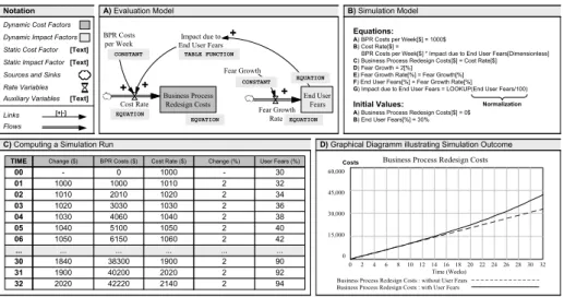
Fig. 7A shows a simple2evaluation model. Assume that the evolution of a DCF ”Busi- ness Process Redesign Costs” caused by the dynamic ImF ”End User Fears” shall be analyzed. Such end user fears can lead to emotional resistance of users, and, in turn, to a lack of support from the users while redesigning business processes, e.g., during an interview-based process analysis.
A) Evaluation Model
C) Computing a Simulation Run
TIME Change ($) BPR Costs ($)
00 - 0
01 1000 1000
02 1010 2010
03 1020 3030
04 1030 4060
05 1040 5100
06 1050 6150
... ... ...
30 1840 38300
31 1900 40200
32 2020 42220
Notation
Flows Auxiliary Variables Rate Variables Dynamic Cost Factors
Links Sources and Sinks Dynamic Impact Factors
[Text]
[+|-]
Static Cost Factor [Text]
Static Impact Factor[Text]
TABLE FUNCTION
EQUATION
Business Process Redesign Costs 60,000
45,000
30,000
15,000
0
0 2 4 6 8 101214161820 22 24 26 28 3032
Time (Weeks) Business Process Redesign Costs : without User Fears Business Process
Redesign Costs
End User Fears Fear Growth
Rate Cost Rate
Impact due to End User Fears BPR Costs
per Week
Fear Growth
B) Simulation Model Equations:
A) BPR Costs per Week[$] = 1000$
B) Cost Rate[$] =
BPR Costs per Week[$] * Impact due to End User Fears[Dimensionless]
C) Business Process Redesign Costs[$] = Cost Rate[$]
D) Fear Growth = 2[%]
E) Fear Growth Rate[%] = Fear Growth[%]
F) End User Fears[%] = Fear Growth Rate[%]
G) Impact due to End User Fears = LOOKUP(End User Fears/100) Initial Values:
A) Business Process Redesign Costs[$] = 0$
B) End User Fears[%] = 30%
Cost Rate ($) 1000 1010 1020 1030 1040 1050 1060 ...
1900 2020 2140
Change (%) - 2 2 2 2 2 2 ...
2 2 2
User Fears (%) 30 32 34 36 38 40 42 ...
90 92 94
D) Graphical Diagramm illustrating Simulation Outcome
Business Process Redesign Costs : with User Fears Costs
CONSTANT
CONSTANT EQUATION
EQUATION EQUATION
Normalization
+ + +
+
Fig. 7. Dealing with the Impact of End User Fears.
Assume that the business process redesign activities are scheduled for 32 weeks. In order to simulate the evolution of the resulting costs along this time frame, we use the
2Note that it is the basic goal of this example to illustrate the simulation of our evaluation models. Usually, evaluation models are more complex. However, due to lack of space we cannot give a more extensive example.
simulation model depicted in Fig. 7B. The nonlinear impact of end user fears on the DCF is represented through a table function. Fig. 7C shows the values of the evaluation model’s dynamic evaluation factors over time when executing the simulation model.
Fig. 7D shows the outcome of the simulation. As can be seen, there is a significant negative impact of end user fears on the costs of business process redesign.
4 Summary
Our paper has illustrated the use of simulation to investigate the dynamic implications described by EcoPOST evaluation models. We have motivated the use of simulation as a means to analyze the dynamic effects caused by feedback loops. We have described the constituting elements of EcoPOST simulation models and have discussed the execution of simulation models. Finally, we have given an illustrating example.
References
1. Reichert, M., Rinderle, S., Kreher, U., Dadam, P.: Adaptive Process Management with ADEPT2. Proc. 21th ICDE ’05, pp.1113-1114 (2005)
2. Dumas, M., van der Aalst, W.M.P., ter Hofstede, A.H.: Process-aware Information Systems:
Bridging People and Software through Process Technology. Wiley (2005)
3. Reijers, H.A., van der Aalst, W.M.P.: The Effectiveness of Workflow Management Systems - Predictions and Lessons Learned. Int’l. J. of Inf. Manag., 25(5), pp.457-471 (2005) 4. Choenni, S., Bakkera, R., Baetsa, W.: On the Evaluation of Workflow Systems in Business
Processes. Electronic Journal of IS Evaluation (EJISE), 6(2) (2003)
5. Oba, M., Onoda, S., Komoda, N.: Evaluating the Quantitative Effects of Workflow Systems based on Real Cases. Proc. 33rd HICSS (2000)
6. Kleiner, N.: Can Business Process Changes Be Cheaper Implemented with Workflow- Management-Systems? Proc. IRMA ’04, pp.529-532 (2004)
7. Mutschler, B., Reichert, M.: A Survey on Evaluation Factors for Business Process Manage- ment Technology. Technical Report, TR-CTIT-06-63, University of Twente (2006) 8. Mutschler, B., Reichert, M., Bumiller, J.: An Approach for Evaluating Workflow Manage-
ment Systems from a Value-Based Perspective. Proc. 10th IEEE EDOC, pp.477-482 (2006) 9. Mutschler, B., Reichert, M.: Analyzing the Dynamic Cost Factors of Process-aware Infor-
mation Systems: A Model-based Approach. Proc. CAiSE ’07 (2007)
10. Richardson, G.P., Pugh, A.L.: System Dynamics - Modeling with DYNAMO. (1981) 11. Forrester, J.W.: Industrial Dynamics. Productivity Press, Cambridge, London (1961) 12. Sterman, J.D.: Business Dynamics - Systems Thinking and Modeling. McGraw-Hill (2000) 13. Mutschler, B., Reichert, M., Bumiller, J.: Designing an Economic-driven Evaluation Frame-
work for Process-oriented Software Technologies. Proc. 28th ICSE, pp.885-888 (2006) 14. Jensen, F.V.: Bayesian Networks and Decision Graphs. Springer (2002)
15. Brassel, K.H., Mhring, M., Schumacher, E., Troitzsch, K.G.: Can Agents Cover All the World? Simulating Social Phenomena, LNEMS 456, Springer (1997)
16. Scholl, H.J.: Agent-based and System Dynamics Modeling: A Call for Cross Study and Joint Research. Proc. 34th Int’l. Conf. on System Sciences (2001)
17. Ogata, K.: System Dynamics. Prentice Hall (2003)
18. Boehm, B., Abts, C., Brown, A.W., Chulani, S., Clark, B.K., Horowitz, E., Madachy, R., Reifer, D., Steece, B.: Software Cost Estimation with Cocomo 2. Prentice Hall (2000) 19. Mutschler, B., Reichert, M., Bumiller, J.: Why Process-Orientation is Scarce: An Emp. Study
of Process-oriented IS in the Autom. Industry. Proc. 10th IEEE EDOC, pp.433-438 (2006)