Housing and Macroeconomy: The Role of Credit Channel, Risk -, Demand - and Monetary Shocks

July 29, 2016

Housing and Macroeconomy: The Role of Credit Channel, Risk -, Demand - and Monetary Shocks

Abstract

This paper demonstrates that risk (uncertainty) along with the monetary (interest rates) shocks to the housing production sector are a quantitatively important impulse mechanism for the business and hous- ing cycles. Our model framework is that of the housing supply/banking sector model as developed in Dorofeenko, Lee, and Salyer (2014) with the model of housing demand presented in Iacoviello and Neri (2010). We examine how the factors of production uncertainty, nancial intermediation, and credit con- strained households can a ect housing prices and aggregate economic activity. Moreover, this analysis is cast within a monetary framework which permits a study of how monetary policy can be used to mitigate the deleterious e ects of cyclical phenomenon that originates in the housing sector. We provide empirical evidence that large housing price and residential investment boom and bust cycles in Europe and the U.S.

over the last few years are driven largely by economic fundamentals and nancial constraints.We also nd that, quantitatively, the impact of risk and monetary shocks are almost as great as that from technology shocks on some of the aggregate real variables. This comparison carries over to housing market variables such as the price of housing, the risk premium on loans, and the bankruptcy rate of housing producers.

JEL Classi cation: E4, E5, E2, R2, R3

Keywords: hetrogenous households, residential investment, housing prices, credit constraint, loan to value ratio, cash in advance constraint, monetary policy, uncertainty and demand shocks

Victor Dorofeenko

Department of Economics and Finance Institute for Advanced Studies

Stumpergasse 56 A-1060 Vienna, Austria

Gabriel S. Lee (Corresponding Author) University of Regensburg

Universtitaetstrasse 31 93053 Regensburg, Germany And

Institute for Advanced Studies Kevin D. Salyer

Department of Economics University of California Davis, CA 95616, U.S.A.

Johannes Strobel University of Regensburg Universtitaetstrasse 31 93053 Regensburg, Germany Contact Information:

Lee: ++49.941.943.5060; E-mail: gabriel.lee@ur.de Salyer: ++1.530.752.8359; E-mail: kdsalyer@ucdavis.edu

We bene tted from comments received during presentations at: the Humboldt University, University of Erlangen-Nuremberg, Computing in Economics and Finance Conference 2014. We are especially indebted to participants in the IHS and the University of Regensburg Macroeconomics Seminars for insightful suggestions that improved the exposition of the paper. We also gratefully acknowledge nancial support from Deutsche Forschungs-

1 Introduction

Figure 1 shows the dramatic rise and fall of real housing prices for the U.S. and some of the selected European countries¹ from the rst quarter of 1997 to the second quarter of 2011. The U.S. housing market peaked in the second quarter of 2007 with the price appreciation of 122 percent.² In comparison to Ireland (300 percent), Greece (185 percent), and Spain (163 percent) and with each country having slightly di erent peak periods, the U.S. housing price appreciation is not only in-line with the rest of the economies but also is relatively mild³. With the subsequent pronounced decline in house prices in these economies from their peaks during the mid 2000's, there is a growing body of literature that describes these large swings in housing prices asbubbles or these sharp increases in housing prices were caused byirrational exuberance⁴, and subsequently, these housing price bubbles then are the causes of the recent global nancial instability.

Given the recent macroeconomic experience of most developed countries, few students of the economy would argue with the following three observations: 1. Financial intermediation plays an important role in the economy, 2. The housing sector is a critical component for aggregate economic behavior and 3. Uncertainty, and, in particular, time-varying uncertainty⁵ - and mon- etary shocks are quantitatively important sources of business cycle activity. And while there has no doubt been a concomitant increase in economic research which examines housing markets and nancial intermediation, only a few analyses have been conducted in a calibrated, general equi- librium setting; i.e. an economic environment in which the quantitative properties of the model

1 We have selected Ireland, Spain, Greece, Italy and Portugal for our illustration purpose. Moreover, these countries are purposely chosen as most of them are currently experiencing a great nancial di culties. We also include Germany, who has not experienced any housing or nancial crisis, to use as a benchmark comparison.

2Unlike the Case-Shiller index that has an appreciation of 122 percent, the O ce of Federal Housing Enterprise Oversight (OFHEO) experienced 77 percent appreciation. The di erence between the The O ce of Federal Housing Enterprise Oversight (OFHEO) and Case-Shiller housing price indices arises largely from the treatment of expensive homes. The OFHEO index includes only transactions involving mortgages backed by the lenders it oversees, Fannie Mae and Freddie Mac, which are capped at $417,000. The Case-Shiller measure has no upper limit and gives more weight to higher-priced homes.

3The following countries have experienced less of an appreciation: Portugal (44 percent), Italy (70 percent) and Germany (-4.2 percent) with even depreciation.

4 The term Irrational Exuberance was rst coined by Alan Greenspan, the former chairman of the Board of Governors of the Federal Reserve in 1996 at the U.S. Congress testimony.

5We de ne and estimate these uncertainty (risk) shocks as the time variation in the cross sectional distribution of rm level productivities. The detail analysis of the risk shock estimation follows in the later section.

are broadly consistent with observed business cycle characteristics with various shocks.⁶ The objective of our paper is to develop a theoretical and computational framework that can help us understand: [1] how does uncertainty in lending channel e ect economies (including both nancial and housing markets) at di erent stages of business cycle; [2] what are the e cts associated with credit constrained heterogenous agents on the housing prices and the business cycle; and [3] what types monetary policies might help (or hinder) the process of housing and nancial development.

To address the aforementioned questions, we use the framework of the housing supply/banking sector model as developed in Dorofeenko, Lee, and Salyer (2014) with the model of housing demand presented in Iacoviello and Neri (2010). In particular, we examine how the factors of production uncertainty, nancial intermediation, and credit constrained households can a ect housing prices and aggregate economic activity. Moreover, this analysis is cast within a monetary framework of Carlstrom and Fuerst (2001) which permits a study of how monetary policy can be used to mitigate the deleterious e ects of cyclical phenomenon that originates in the housing sector.

The Dorofeenko, Lee, and Salyer (2014) model focuses on the e ects that housing production uncertainty and bank lending have on housing prices. To do this, their analysis combines the multi- sector housing model of Davis and Heathcote (2005) with the Carlstrom and Fuerst (1997) model of lending under asymmetric information and agency costs since both models had been shown to replicate several key features of the business cycle. In particular, the Davis and Heathcote (2005) model produces the high volatility of residential investment relative to xed business investment seen in the data. However, the model fails to produce the observed volatility in housing prices.

To this basic framework, Dorofeenko, Lee, and Salyer (2014) introduce an additional impulse mechanism, time varying uncertainty (i.e. risk shocks) shocks to the standard deviation of the entrepreneurs' technology shock a ecting only the housing production, and require that housing

6 Some of the recent works which also examine housing and credit are: Iacoviello and Minetti (2008) and Iacoviello and Neri (2010) in which a new-Keynesian DGSE two sector model is used in their empirical analysis;

Iacoviello (2005) analyzes the role that real estate collateral has for monetary policy; and Aoki, Proudman and Vliegh (2004) analyse house price ampli cation e ects in consumption and housing investment over the business cycle. None of these analyses use risk shocks as an impulse mechanism. Some recent papers that have examined the e ects of uncertainty in a DSGE framework include Bloom et al. (2012), Fernandez-Villaverde et al. (2009), Christiano et al. (2015), and Dorofeenko, Lee and Salyer (2014) with housing markets.

producers nance the purchase of their inputs via bank loans. Dorofeenko, Lee, and Salyer (2014) model risk shocks as a mean preserving spread in the distribution of the technology shocks a ecting only house production and explore quantitatively how changes in uncertainty a ect equilibrium characteristics.⁷ The importance of understanding how these uncertainty or risk shocks a ect the economy is widely discussed in academics and among policymakers. For example, Baker, Bloom, and Davis (2012) demonstrates that a long persistent sluggish economic recovery in the U.S. (e.g.

low output growth and unemployment hovering above 8%) even after the bottoming of the U.S.

recession in June 2009 could be attributed to the high levels of uncertainty about economic policy.

In Dorofeenko, Lee, and Salyer (2014), these factors lead to greater house price volatility as housing prices re ect potential losses due to bankruptcy for some housing producers. In fact, the model is roughly consistent with the cyclical behavior of residential investment and housing prices as seen in U.S. data over the sample period 1975-2010. However, Dorofeenko, Lee, and Salyer (2014) model is not consistent with the behavior of housing prices and rm bankruptcy rates as seen in the recent decade. This failure is not surprising since the role of shocks to housing demand combined with changes in household mortgage nance are not present. Consequently, in this paper, we embed key features of the recent model by Iacoviello and Neri (2010) to rectify this omisssion. As detailed below, the main features of the Iacoviello and Neri (2010) model that we employ are the introduction of heterogenous agents (patient and impatient), a borrowing constraint (which a ects impatient households) and a monetary authority that targets in ation via interest rate. We then introduce housing demand shocks (via preferences) and examine how these get transmitted to the economy. Next we examine optimal monetary policy in this setting.

In analyzing the role of the LTV (Loan to Value) ratio on macro and housing variables, we present three di erent scenarios that are based on LTV ratio: low (80), middle (85) and high (90) borrowing constraints. These di erent levels of LTV ratio are, for an expositional purpose, to

7 One should note that the time varying risk shocks in this paper are quite di erent than the pure aggregate or sectoral technology (supply) shocks. First, risk shocks a ect only the housing production sector. Second, risk shocks are meant to represent the second moments of the variance. That is, these time varying risk shocks proxy the changes in eocnomic environment uncertainty.

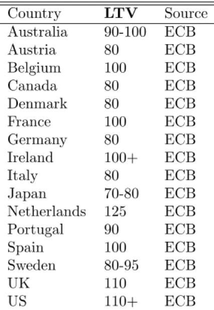
re ect three di erent European economies: Germany, Italy and Spain. According to IMF (2011) (also shown in Table 5 in the Appendix), Germans have one of the lowest LTV ratio, whereas Spanish borrowers have one of the highest LTV ratio with Italy being in between these two levels.⁸

HERE I NEED TO WRITE SOMETHING ELSE OR UPDATE THE RESULTS!!!!

Unlike some of the recent literature that emphasize the important role of the level of LTV on housing market, our results indicate otherwise: almost no di erences between di erent levels of LTV on the variables that we analyze. On the role of speci shocks, we show that the e ects of monetary shocks are huge on most of the macro variables and in particular on the housing investment and the amount of borrowing the households undertake: over 75 percent and almost 50 percent of the variation in housing investment and borrowing can be explained by the monetary shocks. On the contrary to monetary shocks, housing demand shocks have a trivial impact on all the variables that we analyze: at most 6 percent of the variation in housing price can be explained by the preference shocks. Lastly, our endogenous debt nancial accelerator model with risk shocks lends a strong support for the important role of risk shocks: over 85 percent of the variation in housing price is due to risk shocks. Our results, thus, show that there is a clear and an important role for the policy makers to smooth housing price and/or housing investment: to calm markets and to provide and restore market con dence.

2 Model: Housing Markets, Financial Intermediation, and Monetary Policy

Our model builds on three separate strands of literature: Davis and Heathcote's (2005) multi- sector growth model with housing, Dorofeenko, Lee and Salyer's (2008, 2014) credit channel model with uncertainty, and Iacoviello and Neri's (2010) model of housing demand. In this paper, however, we do not consider any other New Keynesian economic frictions other than the

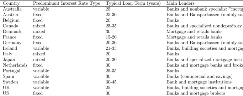
8Some of the recent housing market developments for various European countries are discussed in the Appendix.

asymmetric information friction that occurs in the loan contract between the mutual fund and entrepreneurs.

First we specify the households' optimization problem in a representative agent economy in which the demand for money is motivated by a cash-in-advance constraint. Then, this environment is modi ed by dividing the households into two groups, patient and impatient (a laIacoviello and Neri's (2010)) . This will introduce a role for household lending and borrowing. We then introduce nancial intermediation ("banking") sector, where the patient households lend savings to bankers, and the bankers then lend to both impatient households and entrepreneurs (housing producing agents). With the banking sector, the state of the economy (which is measured in this paper by the level of "uncertaity" or "risk") e ects the lending amount and the probability of loan default, and hence e ecting the net worth of these nancial intermediaries. And consequently, the endogenous net worth of the nanical intermediary sector could in fact contribute aggregate movements in various nancial and macro variables. Finally, we include government in setting monetary policy rule with a variation of the Taylor Rule.

Here is a brief outline and summary of the environment of this economy: Figure 2 shows a schematic of the implied ows for this economy.

Three types of agents:

{ Risk-averse patient (impatient) households that choose consumption, labor, money holding, and housing service: Lend (borrow) money to (from) the nancial intermedi- aries.

{ Risk-neutral entrepreneurs (housing developers) that choose consumption, investment, and labor.

Cost of inputs is nanced by borrowing Housing production subject to risks shocks.

Multisectors: 6 Firms

{ Threeintermediate goods producing: Construction, Manufacturing, and Service

{ Two" nal" goods production: Residential Investment and Consumption / Non-residential Investment

{ HousingProduction (via entrepreneurs): Residential Investment + Land.

A mutual fund: Financial intermediaries (that guarantees a certain return to house- holds through lending to an in nite number of entrepreneurs).

Government: Lump sum money transfer and taxes.

Shocks: 6 di erent shocks

{ 3 sectoral productivity technology shocks: Construction, Manufacturing and Service { Idiosyncratic technology shocks (!t) a ecting housing production.

Denoting thec:d:f:andp:d:f:of !tas (!t; !;t) and (!t; !;t).

Second moment, !;t;(i.e. risk) shocks a ecting the distribution of these Idiosyn- cratic technology shocks.

{ Monetary shocks: a la Taylor Rule.

{ Housing demand (preference) shocks.

2.1 Money and cash-in-advance constraint in housing model: House- holds

This section follows the work of Carlstrom and Fuerst (2001) but adds loans and collateral restric- tions on the demand side as in Iacoviello and Neri (2010). Households maximize lifetime utility given by:

E0

X1 t=0

tU(ct; ht;1 Nt)

!

(1)

w.r.t. its consumption c_t, labor hours N_t, capitalK_t and housingh_tstocks, the investment into consumption ik;t and housing ih;t goods sectors, and money holdings Mt subject to the budget constraint (where we let to denote the Lagrange multiplier):

ct+ik;t+ph;tih;t+Mt+1

Pc;t

(2) K_t(r_{t k}(r_{t k})) +N_tw_t(1 _n) +p_l;tx_l;t+M_t+M_s;t

Pc;t

:

Pc;t denotes the nominal consumption price. Note that the new monetary injection, Ms;t is distributed by the government at the beginning of the period as a lump-sum transfer (with the aggregate money stock given byMs;t): The cash-in-advance constraint (CIA) states that money (post-transfer) must be used to buy investment and consumption goods (the associated Lagrange multiplier is ):

c_t+i_k;t+p_h;ti_h;t M_t+M_s;t Pc;t

(3)

The laws of motion for capital and housing are given by (the respective Lagrange multipliers are and ):

Kt+1=Fk(ik;t; ik;t 1) + (1 k)Kt (4)

ht+1=Fh(ih;t; ih;t 1) + (1 h)ht (5)

Here _k and _n are the capital income and labor income taxes correspondingly, represents the usual capital/housing depreciation rate,p_l;tx_l;tis the value of land, and the functionF_j(i_j;t; i_{j;t 1}) accounts investment adjustment cost. According to Christiano et. al (2005), F_j(i_j;t; i_{j;t 1}) =

1 S _i^ij;t

j;t 1 i_j;t, where S(1) =S⁰(1) = 0 andS⁰⁰(1)>0.

The correspondent Euler equations are:

U1t t t= 0

w_{t t} U_3t= 0

t= Et((1 k) t+1+ ((1 k)rt+1+ k k) t+1)

t= Et((1 h) t+1+U2t+1)

t+ t= tFc;1(ik;t; ik;t 1) + Et( t+1Fc;2(ik;t+1; ik;t)) p_{h; t}( _t+ _t) = _tF_h;1(i_{h; t}; i_{h; t 1}) + E_t( _t+1F_h;2(i_{h; t+1}; i_{h; t}))

t

P_c;t = E_t ^t+1+ _t+1 P_c;t+1

Introducing the nominal interest rate Rt and the shadow prices of the capital and housing good,qkt andqh;t respectively:

Rt= 1 + ^t

t

; t=qk;tU1;t; t=qh;tU1;t

we obtain:

w_t R_t = U_3t

U_1t (6)

qk;t= Et (1 k)qk;t+1+(1 k)rt+1+ k k

R_t+1

U1;t+1

U_1;t (7)

qh;t= Et (1 h)qh;t+1

U1;t+1

U1;t

+U2;t+1

U1;t

(8)

1 =q_k;tF_k;1(i_{k; t}; i_{k; t 1}) + E_t q_k;t+1F_k;2(i_{k; t+1}; i_{k; t})U_1;t+1 U1;t

(9)

ph; t=qh;tFh;1(ih; t; ih; t 1) + Et qh;t+1Fh;2(ih; t+1; ih; t)U1;t+1

U_1;t (10)

including the Fisher equation for the nominal interest rate:

1 = R_tE_t U_1;t+1 (1 + t+1)U1;t

(11)

where we introduce the in ation rate _t,

t+1= Pc;t+1

P_c;t 1

The substitution of (3) into (2) and assuming that both constraints are binding, we have our budget constraint as:

c_t+1+i_k;t+1+p_h;t+1i_h;t+1= (12)

Kt((1 k)rt+ k k) +Ntwt(1 n) +pl;txl;t

1 + t+1

+Ms;t+1

Pc;t+1

2.1.1 Utility function and demand shocks The utility function is assumed to have the form:

U(c; h; l) =(c ^ch ^hl ^l)¹

1 (13)

where denotes the coe cient of relative risk aversion. The housing demand shock can be added to the utility function assuming that the parameter _h follows the AR(1) processes:

ln h;t+1= (1 h) ln ⁽⁰⁾_h + hln h;t+"h;t+1 (14)

We use, in fact, the same utility function as Devis and Heathcote (2005), but slightly deviate from them in notation ( l 6= 1 c h;t) to avoid the in uence of housing demand shocks on the labor supply share l.

2.1.2 Heterogeneous agents, borrowing and collateral constraint at the demand side As in Iacoviello and Neri (2010), we now introduce two types of agents, patient and impatient. A prime is used to denote impatient household's parameters and variables ( ⁰; N⁰ etc.). The patient

households as described in the previous section have a discount factor that is larger than the impatient ones, > ⁰. While both groups may lend or borrow money, the assumption > ⁰ will always lead to the situation where the patient households lend money to the impatient ones.

Adding the borrowingbtto the patient household's budget constraint (2) produce the inequality (lending corresponds to the negative values ofbt):

c_t+i_k;t+p_h;ti_h;t+b_{t 1}R_{b;t 1} 1 + t

+M_t+1 Pc;t

(15) Kt(rt k(rt k)) +Ntwt(1 n) +pl;txl;t+bt+Mt+Ms;t

P_c;t

In addition to the budget constraint, households face a cash-in-advance constraint:

ct+ik;t+ph;tih;t

M_t+M_s;t Pc;t

(16)

so, the relation (12) is changed to the form:

ct+1+ik;t+1+ph;t+1ih;t+1= (17)

Kt(rt k(rt k)) +Ntwt(1 n) +pl;txl;t+bt Rb;t 1bt 1

1+ t

1 + _t+1 +aMms;t+1

where ms;t = Ms;t+M_s;t⁰ =Pc;t. The share aM = Ms;t= Ms;t+M_s;t⁰ is chosen equal to its steady-state value and remains constant.

The impatient households have shorter budget constraint, because they don't own capital and land, so the quantities proportional toK_t,i_kt andx_lt are omitted:

c⁰_t +p_h;ti⁰_h;t+R_{b;t 1}b⁰_{t 1} 1 + _t +M_t+1⁰

P_c;t =N_t⁰w_t⁰(1 _n) +b⁰_t+M_t⁰+M_s;t⁰

P_c;t (18)

and their CIA constraint is:

c⁰_t +ph;ti⁰_h;t M_t⁰+M_s;t⁰

P_c;t (19)

which leads to the combined constraint:

c⁰_t+1 +p_h;t+1i⁰_h;t+1= N_t⁰w_t⁰(1 n) +b⁰_t ^Rb;t₁₊^{1b0t 1}

t

1 + t+1

+ (1 a_M)m_s;t+1 (20)

The additional (binding) borrowing constraint for the impatient households (collateral con- straint) restricts the size of the borrowed funds by the value of their housing stock:

b⁰_t mEt

ph;t+1(1 + t+1)h⁰_t

R_t (21)

wheremdenotes the loan-to-value (LTV) ratio. Iacoviello and Neri (2010) setmfor the impatient fraction of the USA households equal to m = 0:85. In our calibration exercise, we vary in the range from 0:1 to 0:9 to analyse the e ects ofmon our economy;m=f0:1;0:8;0:85;0:9g:

The market clearing condition for the borrowing is:

b⁰_t+bt= 0 (22)

The housing stock growth equations for the patient and impatient householders are:

h_t+1+h⁰_t+1=F_h(i_{h; t}; i_{h;t 1}) +F_h i⁰_{h; t}; i⁰_{h;t 1} + (1 _h) (h_t+h⁰_t) (23)

The patient households maximize their lifetime utility (1) w.r.t. consumptionc_t, labor hours N_t, capital K_t and housing h_t stocks, the investment into consumption i_k;t and housing i_h;t goods sectors, money holdings Mt and borrowingbt subject to constraints (15) and (16), stock accumulation equation (23) and the capital growth equation (4)

Their Euler equations consist of system (6) - (11) and the additional equation for the borrowing interest rate rb;t:

1 = Rb;tEt

Rt

R_t+1

U1;t+1

(1 + _t+1)U_1;t (24)

The impatient households maximize their lifetime utility (1) w.r.t. consumptionc⁰_t, labor hours N_t⁰, housingh⁰_t, the investment into housing goods sectori⁰_{h; t}, money holdingsM_t⁰and borrowingb⁰_t subject to constraints (18), (19), collateral constraint (21) and the housing accumulation equation (??). Their Euler equations are:

w⁰_t R⁰_t = U_3t

U_1t (25)

1 = ⁰R⁰_tEt

U1;t+1

(1 + _t+1)U_1;t (26)

q_b;t⁰ R⁰_t= 1 ⁰Rb;tEt

R⁰_t R_t+1⁰

U_1;t+1 (1 + t+1)U1;t

(27)

q_h;t⁰ = ⁰Et (1 h)q_h;t+1⁰ +q⁰_b;t+1b⁰_t+1 h⁰_t+1

U_1;t+1 U1;t

+U_2;t+1 U1;t

(28)

p_{h; t}=q⁰_h;tF_h;1 i⁰_{h; t}; i⁰_{h;t 1} + ⁰E_t q⁰_h;t+1F_h;2 i⁰_{h; t+ 1}; i⁰_h;t U1;t+1

U_1;t (29)

Here q_b;t⁰ denotes the shadow price of borrowing. The utility function U =U(c⁰_t;1 N_t⁰; h⁰_t) in equations (25) - (29) depends on the impatient household's consumption c⁰_t, labor hoursN_t⁰ and housingh⁰_t.

2.2 Production (Firms): with only one household

We rst assume a representative agent framework and then introduce heterogeneous agents as described above. We assume (as in Davis and Heathcote (2005)) that nal goods (residential investment and consumption goods) are produced using intermediate goods. The intermediate goods sector consists of three output: building/construction, manufacture, and services, which

are produced via Cobb-Douglas production functions:

xi=k_iⁱ(e^zini)^{1 i} (30)

wherei=b; m; s(building/construction, manufacture, service),kit; nitandzitare capital, house- hold -, entrepreneur labor, and labor augumenting (in log) productivity shock respectively for each sector, with the _ibeing the share of capital that di er across sectors. For example, we let in our calibration that _b< _m;re ecting the fact that the manufacturing sector is more capital in- tensive (or less labor intensive) than the construction sector. Unlike Davis and Heathcote (2005), we include entrepreneurial labor supply in the production function.⁹

The production shocks grows linearly:

zi=tlngz;i+ ~zi (31)

with the stochastic term~z= (~z_b;z~_m;z~_s) following the vectorAR(1) process:

~

z_t+1=B ~z_t+~"_t+1 (32)

where the the matrix B captures the deterministic part of shocks over time, and the innovation vector~"is distributed normally with a given covariance matrix ". The shock growth factorsgz;i

lead to the correspondent growth factors for other variables.

These intermediate rms maximize a conventional static pro t function att

max

fkit;nitg

(X

i

p_itx_it r_tk_t w_tn_t )

(33)

9Although we do not include in the model the entrepreneurial labor income, the assumption of entrepreneurial labor income is necessary as it gurantees a nonzero net worth for each entrepreneur. This nonzero net worth assumption is important as the nancial contracting problem is not well de ned otherwise. In our calibration section, we let the share of entrepreneur's labor supply to be quite small but nonzero. Consequently, although the entreprenuers' labor supply do not play a role in our equilibrium conditions, small share of entrepreneur's labor supply does ensure a small but nonzero net worth.

subject to equationsk_t P

ik_it; n_t P

in_it;and non-negativity of inputs, where r_t; w_t, and p_it are the capital rental, wage, and output prices. A conventional optimization leads to the relations:

kir= ipixi (34)

niw= (1 i)pixi (35)

so that

k_ir+n_iw=p_ix_i (36)

The intermediate goods are then used as inputs to produce two nal goods,yj:

yjt=

i=b;m;sx1_ijt^ij; (37)

wherej=c; d(consumption/capital investment and residential investment respectively), the input matrix is de ned by

x1 = 0 BB BB BB

@

bc bd

mc md

sc sd

1 CC CC CC A

; (38)

and the shares of construction, manufactures and services for sectorj are de ned by the matrix

= 0 BB BB BB

@

Bc Bd

M_c M_d S_c S_d

1 CC CC CC A

: (39)

The relative shares of the three intermediate inputs di er in producing two nal goods. For example, we would set Bc < Bd to represent the fact that the residential investment is more construction input intensive. Moreover, with the CRS property of the production function, the

following conditions must also be satis ed:

X

i

ij = 1 (40)

and

xit=X

j

x1ijt (41)

i.e

x_bt=b_ct+b_dt; x_mt=m_ct+m_dt; x_st=s_ct+s_dt: (42)

With intermediate goods as inputs, the nal goods' rms solve the following static pro t maximization problem att where the price of consumption good,pct;is normalized to 1:

fbjt;maxmjt;sjtg

(

yct+pdtydt

X

i

pitxit

)

subject to equation (37) and non-negativity of inputs. The optimization of nal good rms leads to the relations:

p_itx1_i;jt= _i;jp_jty_jt (43)

where i=b; m; s, j=c; d

Due to CRS property, we obtain:

X

i=b;m;s

pitxit= X

j=c;d

pjtyjt=Ktrt+wtNt (44)

where

K_t= X

i=b;m;s

k_it; N_t= X

i=b;m;s

n_it (45)

Lastly, the housing rms (real estate developers or entrepreneurs) produce the housing good,

y_ht, given residential investmenty_dtand x amount of landx_lt as inputs, according to

yht=x_lty¹_dt (46)

where, denotes the share of land. Output equation (46) will be modi ed later in the section to include idiosyncratic productivity and uncertainty shocks. As mentioned in the introduction, the focus of our paper is on the housing sector in which agency costs with uncertainty and hetroe- geneity arise: we come back to this modi cation on the rms' behaviorin the later section. The optimization de nes the price relations:

plxl= phyh; pdyd= (1 )phyh (47)

2.2.1 Firms: Production side with two types of households

With both patient and impatient household, we now need to make small modi cations of the production side of the model due to the presence of two types of labor supplying households in the system. Now the production of the intermediate good (30) changes to the form¹⁰:

xi=k_iⁱ e^zin^a_in⁰_i^{1 1 i} (48)

where n_i and n⁰_i are the hours supplied by the patient and impatient households respectively accordingly to their labor share . Equations (35) and (36) now are:

niw= pixi(1 i) (49)

n⁰_iw⁰= (1 )pixi(1 i) (50)

10For the simplicity purpose, we drop the time script in this section.

and

kir+n⁰_iw⁰+niw=pixi: (51)

Balance equations (44) are also changed to:

X

i=b;m;s

pixi = X

j=c;d

pjyj=Kr+N w+N⁰w⁰: (52)

The new variableN⁰ denotes the total impatient household's hours:

N⁰= X

i=b;m;s

n⁰_i: (53)

We can introduce now the e ective hoursLand the e ective wage W:

L=N N⁰¹ ; W = w w⁰ 1

1

: (54)

Then from relation (49) and (50) follows that

LW =N w+N⁰w⁰: (55)

We can also introduce the e ective hours li = n_in⁰_i¹ for building, manufacture and services (i=b; m; s) separately:

li=n_in⁰_i¹ :

Then the following equations hold:

l_iW = (1 _i)p_ix_i=n⁰_iw⁰+n_iw; L= X

i=b;m;s

l_i

2.3 Credit Channel with Uncertainty

In this section, we outline how the nancial intermediaries decide on the amount of loan that is to be lend out to housing developers (entrepreneurs). One should note that in our lending model, we only focuses on the supply side. That is, we do not address the endogenous lending mechanism for the impatient households (the demand side): The loan for the impatient household is exogenously determined by the collateral constraint in equation (21).

2.3.1 Housing Entrepreneurial Contract

It is assumed that a continuum of housing producing rms with unit mass are owned by risk- neutral entrepreneurs (developers). The costs of producing housing are nanced via loans from risk-neutral intermediaries. Given the realization of the idiosyncratic shock to housing production, some real estate developers will not be able to satisfy their loan payments and will go bankrupt.

The banks take over operations of these bankrupt rms but must pay an agency fee. These agency fees, therefore, a ect the aggregate production of housing and, as shown below, imply an endogenous markup to housing prices. That is, since some housing output is lost to agency costs, the price of housing must be increased in order to cover factor costs.

The timing of events is critical:

1. The exogenous state vector of technology shocks, uncertainty shocks, housing preference shocks, and monetary shocks, denoted (z_i;t; _!;t; _h;t+1; R_t+1), is realized.

2. Firms hire inputs of labor and capital from households and entrepreneurs and produce intermediate output via Cobb-Douglas production functions. These intermediate goods are then used to produce the two nal outputs.

3. Households make their labor, consumption, housing, and investment decisions.

4. With the savings resources from households, the banking sector provide loans to entrepreneurs via the optimal nancial contract (described below). The contract is de ned by the size of

the loan (f p_at) and a cuto level of productivity for the entrepreneurs' technology shock,

!t.

5. Entrepreneurs use their net worth and loans from the banking sector in order to purchase the factors for housing production. The quantity of factors (residential investment and land) is determined and paid for before the idiosyncratic technology shock is known.

6. The idiosyncratic technology shock of each entrepreneur is realized. If !at !t the en- trepreneur is solvent and the loan from the bank is repaid; otherwise the entrepreneur declares bankruptcy and production is monitored by the bank at a cost proportional (but time varying) to total factor payments.

7. Solvent entrepreneur's sell their remaining housing output to the bank sector and use this income to purchase current consumption and capital. The latter will in part determine their net worth in the following period.

8. Note that the total amount of housing output available to the households is due to three sources: (1) The repayment of loans by solvent entrepreneurs, (2) The housing output net of agency costs by insolvent rms, and (3) the sale of housing output by solvent entrepreneurs used to nance the purchase of consumption and capital.

A schematic of the implied ows is presented in Figure 2.

For entrepreneura, the housing production function is denoted G(xalt; yadt) and is assumed to exhibit constant returns to scale. Speci cally, we assume:

y_aht=!_atG(x_alt; y_adt) =!_atx_alty¹_adt (56)

where, denotes the share of land. It is assumed that the aggregate quantity of land is xed and equal to 1. The technology shock, !at, is an idiosyncratic shock a ecting real estate developers.

The technology shock is assumed to have a unitary mean and standard deviation of !;t. The

standard deviation, _!;t;follows anAR(1) process:

!;t+1= ¹_{0 !;t}exp^{" ;t+1} (57)

with the steady-state value 0; 2(0;1) and" ;t+1 is a white noise innovation.¹¹

Each period, entrepreneurs enter the period with net worth given bynwat:Developers use this net worth and loans from the banking sector in order to purchase inputs. Lettingf p_at denote the factor payments associated with developera, we have:

f pat=pdtyadt+pltxalt (58)

Hence, the size of the loan is (f pat nwat): The realization of!at is privately observed by each entrepreneur; banks can observe the realization at a cost that is proportional to the total input bill.

It is convenient to express these agency costs in terms of the price of housing. Note that agency costs combined with constant returns to scale in housing production (see eq. (56)) implies that the aggregate value of housing output must be greater than the value of inputs; i.e. housing must sell at a markup over the input costs, the factor payments. Denote this markup as st (which is treated as parametric by both lenders and borrowers) which satis es:

phtyht=stf pt (59)

Also, sinceE(!_t) = 1 and all rms face the same factor prices, this implies that, at the individual

11This autoregressive process is used so that, when the model is log- linearized, ^!;t(de ned as the percentage deviations from 0) follows a standard, mean-zero AR(1) process.

level, we have¹²

phtG(xalt; yadt) =stf pat (60)

Given these relationships, we de ne agency costs for loans to an individual entrepreneur in terms of foregone housing production as stf pat:

With a positive net worth, the entrepreneur borrows (f pat nwat) consumption goods and agrees to pay back 1 +r^L_t (f p_at nw_at) to the lender, where r^L_t is the interest rate on loans.

The cuto value of productivity, !_t, that determines solvency (i.e. !_at !_t) or bankruptcy (i.e. !_at < !_t) is de ned by 1 +r_t^L (f p_at nw_at) = p_ht!_tF( ) (where F( ) = F(x_alt; y_adt)).

Denoting the c:d:f: and p:d:f: of !tas (!t; !;t) and (!t; !;t), the expected returns to a housing producer is therefore given by:¹³

Z ₁

!t

pht!F( ) 1 +r^L_t (f pat nwat) (!; !;t)d! (61)

Using the de nition of !_tand eq. (60), this can be written as:

s_tf p_atf(!_t; _!;t) (62)

where f(!t; !;t) is de ned as:

f(!t; !;t) = Z ₁

!t

! (!; !;t)d! [1 (!t; !;t)]!t (63)

Similarly, the expected returns to lenders is given by:

Z !t

0

p_ht!F( ) (!; _!;t)d!+ [1 (!_t; _!;t)] 1 +r^L_t (f p_at nw_at) (!_t; _!;t) s_tf p_at (64)

12The implication is that, at the individual level, the product of the markup (st) and factor payments is equal to the expected value of housing production since housing output is unknown at the time of the contract. Since there is no aggregate risk in housing production, we also havephtyht=stf pt:

13The notation (!; !;t) is used to denote that the distribution function is time-varying as determined by the realization of the random variable, !;t.

Again, using the de nition of!_tand eq. (60), this can be expressed as:

stf patg(!t; !;t) (65)

where g(!t; !;t) is de ned as:

g(!_t; _!;t) = Z !t

0

! (!; _!;t)d!+ [1 (!_t; _!;t)]!_t (!_t; _!;t) (66)

Note that these two functions sum to:

f(!t; !;t) +g(!t; !;t) = 1 (!t; !;t) (67)

Hence, the term (!t; !;t) captures the loss of housing due to the agency costs associated with bankruptcy. With the expected returns to lender and borrower expressed in terms of the size of the loan,f p_at; and the cuto value of productivity,!_t;it is possible to de ne the optimal borrowing contract by the pair (f p_at; !_t) that maximizes the entrepreneur's return subject to the lender's willingness to participate (all rents go to the entrepreneur). That is, the optimal contract is determined by the solution to:

!maxt;f pat

stf patf(!t; !;t) subject tostf patg(!t; !;t)>f pat nwat (68)

A necessary condition for the optimal contract problem is given by:

@(:)

@!t

:s_tf p_at@f(!_t; _!;t)

@!t

= _ts_tf p_at@g(!_t; _!;t)

@!t

(69)

where _t is the shadow price of the lender's resources. Using the de nitions of f(!_t; _!;t) and

g(!_t; _!;t), this can be rewritten as:¹⁴

1 1

t

= (!t; !;t)

1 (!_t; _!;t) (70)

As shown by eq.(70), the shadow price of the resources used in lending is an increasing function of the relevant Inverse Mill's ratio (interpreted as the conditional probability of bankruptcy) and the agency costs. If the product of these terms equals zero, then the shadow price equals the cost of housing production, i.e. _t= 1.

The second necessary condition is:

@(:)

@f p_at :stf(!t; !;t) = t[1 stg(!t; !;t)] (71)

These rst-order conditions imply that, in general equilibrium, the markup factor,st;will be endogenously determined and related to the probability of bankruptcy. Speci cally, using the rst order conditions, we have that the markup,s_t;must satisfy:

s_t¹=

"

(f(!_t; _!;t) +g(!_t; _!;t)) + (!t; !;t) f(!t; !;t)

@f(!t; !;t)

@!t

#

(72)

= 2 66

641 (!t; !;t)

| {z }

A

(!t; !;t)

1 (!t; !;t) f(!t; !;t)

| {z }

B

3 77 75

which then can be written as

st= 1

1 ($_t) + f($_t)_f^'($_0($^t)

t)

(73)

We make some brief remarks on the markup equation above. First note that the markup factor depends only on economy-wide variables so that the aggregate markup factor is well de ned. Also,

14Note that we have used the fact that ^@f(^!t; _!;t)

@!_t = (!t; !;t) 1<0

the two terms,AandB, demonstrate that the markup factor is a ected by both the total agency costs (termA) and the marginal e ect that bankruptcy has on the entrepreneur's expected return.

That is, termB re ects the loss of housing output, ;weighted by the expected share that would go to entrepreneur's,f(!t; !;t);and the conditional probability of bankruptcy (the Inverse Mill's ratio). Finally, note that, in the absence of credit market frictions, there is no markup so that st= 1. In the partial equilibrium setting, it is straightforward to show that equation (72) de nes an implicit function!(s_t; _!;t) that is increasing ins_t.

The incentive compatibility constraint implies

f pat= 1

(1 s_tg(!_t; _!;t))nwat (74)

Equation (74) implies that the size of the loan is linear in entrepreneur's net worth so that aggregate lending is well-de ned and a function of aggregate net worth.

The e ect of an increase in uncertainty on lending can be understood in a partial equilibrium setting where s_tandnw_at are treated as parameters. As shown by eq. (72), the assumption that the markup factor is unchanged implies that the costs of default, represented by the termsAand B, must be constant. With a mean-preserving spread in the distribution for!_t, this means that

!twill fall (this is driven primarily by the termA). Through an approximation analysis, it can be shown that !t g(!t; !;t) (see the Appendix in Dorofeenko, Lee, and Salyer (2008)). That is, the increase in uncertainty will reduce lenders' expected return (g(!t; !;t)). Rewriting the binding incentive compatibility constraint (eq. (74)) yields:

s_tg(!_t; _!;t) = 1 nw_at f pat

(75)

the fall in the left-hand side induces a fall inf pat. Hence, greater uncertainty results in a fall in housing production. This partial equilibrium result carries over to the general equilibrium setting.

The existence of the markup factor implies that inputs will be paid less than their marginal products. In particular, pro t maximization in the housing development sector implies the fol- lowing necessary conditions:

plt

pht

= Gxl(xlt; ydt) st

(76) p_dt

pht

= G_yd(x_lt; y_dt) st

(77)

These expressions demonstrate that, in equilibrium, the endogenous markup (determined by the agency costs) will be a determinant of housing prices.

The production of new housing is determined by a Cobb-Douglas production with residential investment and land ( xed in equilibrium) as inputs. Denoting housing output, net of agency costs, as yht;this is given by:

yht=x_lty_dt¹ [1 (!t; !;t) ] (78)

In equilibrium, we require that i_ht=y_ht; i.e. household's housing investment is equal to housing output. Recall that the law of motion for housing is given by eq. (5)

2.3.2 Entrepreneurial Consumption and House Prices

To rule out self- nancing by the entrepreneur (i.e. which would eliminate the presence of agency costs), it is assumed that the entrepreneur discounts the future at a faster rate than the patient household. This is represented by following expected utility function:

E₀P₁

t=0( )^tc^e_t (79)

where c^e_t denotes entrepreneur's per-capita consumption at date t; and 2 (0;1): This new parameter, , will be chosen so that it o sets the steady-state internal rate of return due to housing production.

Each period, entrepreneur's net worth,nw_t is determined by the value of capital income and the remaining capital stock.¹⁵ That is, entrepreneurs use capital to transfer wealth over time (recall that the housing stock is owned by households). Denoting entrepreneur's capital ask_t^e, this implies:¹⁶

nwt=k_t^e[rt+ 1 ] (80)

The law of motion for entrepreneurial capital stock is determined in two steps. First, new capital is nanced by the entrepreneurs' value of housing output after subtracting consumption:

k_t+1^e =phtyahtf(!t; !;t) c^e_t=stf patf(!t; !;t) c^e_t (81)

Note we have used the equilibrium condition thatphtyaht =stf pat to introduce the markup, st, into the expression. Then, using the incentive compatibility constraint, eq. (74), and the de nition of net worth, the law of motion for capital is given by:

k^e_t+1=k^e_t(r_t+ 1 ) s_tf(!_t; _!;t)

1 stg(!t; !;t) c^e_t (82)

The term stf(!t; !;t)=(1 stg(!t; !;t)) represents the entrepreneur's internal rate of return due to housing production; alternatively, it re ects the leverage enjoyed by the entrepreneur since

stf(!t; !;t)

1 stg(!t; !;t) =stf patf(!t; !;t) nwt

(83)

That is, entrepreneurs use their net worth to nance factor inputs of value f p_at; this produces housing which sells at the markups_twith entrepreneur's retaining fractionf(!_t; _!;t) of the value of housing output.

15As stated in footnote 6, net worth is also a function of current labor income so that net worth is bounded above zero in the case of bankruptcy. However, since entrepreneur's labor share is set to a very small number, we ignore this component of net worth in the exposition of the model.

16For expositional purposes, in this section we drop the subscriptadenoting the individual entrepreneur.

Given this setting, the optimal path of entrepreneurial consumption implies the following Euler equation:

1 = Et (rt+1+ 1 ) st+1 f(!t+1; !;t+1)

1 s_t+1g(!_t+1; _!;t+1) (84)

Finally, we can derive an explicit relationship between entrepreneur's capital and the value of the housing stock using the incentive compatibility constraint and the fact that housing sells at a markup over the value of factor inputs. That is, since p_htF(x_alt; y_adt) =s_tf p_t, the incentive compatibility constraint implies:

pht x_lty_dt¹ =k_t^e (rt+ 1 )

1 s_tg(!_t; _!;t)st (85)

Again, it is important to note that the markup parameter plays a key role in determining housing prices and output.

2.3.3 Financial Intermediaries

The Capital Mutual Funds (CMFs) act as risk-neutral nancial intermediaries who earn no pro t and produce neither consumption nor capital goods. There is a clear role for the CMF in this economy since, through pooling, all aggregate uncertainty of capital (house) production can be eliminated. The CMF receives capital from three sources: entrepreneurs sell undepreciated capital in advance of the loan, after the loan, the CMF receives the newly created capital through loan repayment and through monitoring of insolvent rms, and, nally, those entrepreneur's that are still solvent, sell some of their capital to the CMF to nance current period consumption. This capital is then sold at the price of st units of consumption to households for their investment plans.

2.4 Government budget constraint

Assuming the absence of government money holdings, its budget constraint equation is:

G_t+ ($_t)p_h;ty_h;t+m_s;t+m⁰_s;t= (86) Kt(rt k) k+ (Ntwt+N_t⁰w⁰_t) n+m^G_t

where Gt denotes the real government spending, ms;t=Mst=Pc;t; m⁰_s;t = M_t⁰=Pc;t; and m^G_t = M_t^G=P_c;tandM_t^G is a lump-sum money injection into the whole economy. Here we let the money evolves according to

m^G_t+1= (1 _M)m^G₀ + _Mm^G_t

where, M 2(0;1).

Following Christiano, Eichenbaum and Trabandt (2014), we use the monetary policy rule as:

log R_b;t+1 Rb

=%_Rlog R_b;t Rb

+(1 %_R) % log 1 + _t+1

1 + +%_gdplog GDP_t+1

GDP +% _gdplog GDP_t+1 GDPt

+"_R;t+1 (87)

We also use one-period log-di erence for GDP instead of averaged four-period di erence used by Christiano et al, (2014).¹⁷

We assume here that the monitoring of defaulting rms is arranged by a government's insti- tution, but separate the monitoring cost ($t)ph;tyh;t from the other government spendings as each deafulting rms belong to di erent industries (see eqs (89) and (90) below). The share of government spendings Gt=GDPt = aG is considered to be a xed value according to Davis and Heathcote (2005) (see eq (91)). The government distributes money injections M_st and M_st⁰ between the patient and impatient householders proportionally to their steady-state shares M₀

17 Equation (87) contains variables with exponential trend removed. The variables without subscript denote steady-state values. We use \borrowing interest rate" of borrowing between patient and impatient households,Rb

, in eq (87) as one of the targeted values.