Research Collection
Working Paper
Housing Demand Shocks and Households’ Balance Sheets
Author(s):
Anderes, Marc Publication Date:
2021-02
Permanent Link:
https://doi.org/10.3929/ethz-b-000470105
Rights / License:
In Copyright - Non-Commercial Use Permitted
This page was generated automatically upon download from the ETH Zurich Research Collection. For more information please consult the Terms of use.
ETH Library
KOF Working Papers, No. 492, February 2021
Housing Demand Shocks and Households’ Balance Sheets
Marc Anderes
ETH Zurich
KOF Swiss Economic Institute LEE G 116
Leonhardstrasse 21 8092 Zurich, Switzerland Phone +41 44 632 42 39 Fax +41 44 632 12 18 www.kof.ethz.ch kof@kof.ethz.ch
Housing Demand Shocks and Households’ Balance Sheets
Marc Anderes†
KOF Swiss Economic Institute, ETH Zurich February 8, 2021
Abstract
We examine the dynamic effects of housing demand shocks on a large set of U.S. macroeconomic series and detailed household balance sheet components for four wealth percentile groups. The results show that a positive housing shock translates into a large and persistent boom of economic activity, an expansion of credit and an increase of interest rates. While households of all wealth percentile groups make heavy use of home equity-based borrowing, we find a larger consumer spending sensitivity for weaker balance sheet households. This is supported by the elasticities of consumption with respect to house prices implied by our structural dynamic factor model. A historical decomposition suggests that housing demand shocks have largely contributed to the pronounced drop in poorer households’ consumption during the Great Recession.
Variance decompositions indicate that the identified housing shock has high explanatory power for key economic indicators, housing indices and household balance sheet series.
JEL Code: D31, E21, E32, E44, R31
Keywords: Housing demand shocks, Household balance sheets, Bayesian dynamic factor model
†Affiliation: KOF Swiss Economic Institute, ETH Zurich, Leonhardstrasse 21, 8092 Z¨urich, Switzerland. Email: an- deres@kof.ethz.ch. I am grateful to my advisor Jan-Egbert Sturm for his guidance and support. I also thank Sylvia Kaufmann, Samad Sarferaz, Daniel Kaufmann, Alex Rathke, Florian Eckert and Regina Pleninger for very helpful comments. All remaining mistakes are my own. The author declares that he has no relevant or material financial interests that relate to the research described in this paper.
1 Introduction
The financial crisis of 2007-2008 was closely related to the collapse of the U.S. housing market.
Accordingly, a growing literature suggests that housing demand shocks are significant drivers of business cycle fluctuations (Iacoviello and Neri, 2010,Liu et al., 2013).
The tight connection between economic activity and housing is often ascribed to three main channels. The first one stems from Tobin’s q effect, which indicates that rising house prices lead to an increase in real estate values over construction costs, thereby stimulating residen- tial investment which can be a key component of GDP growth (Leamer, 2007). A second transmission channel works via the credit market. A positive housing demand shock increases homeowners assets and thus the value of collateral, mitigating households’ and firms’ credit constraints (Iacoviello, 2005, Mian and Sufi, 2011, Liu et al., 2013). The same balance sheet mechanism applies to the lending side, as financial intermediaries expand credit supply along with the increase of assets held (Adrian et al., 2010). The third channel is an implication of consumption smoothing in life-cycle models. An unexpected and permanent increase of wealth leads households to borrow more and increase consumption. The dynamic interdependence between household balance sheets, the credit market and the housing market is thus able to amplify each channel, possibly making it a powerful driver of real economic activity.
The experience of the Great Recession indicated that the strength of such feedback loops also depends on the heterogeneity of households’ balance sheets. While traditional macroeconomic models assume a representative agent framework in which households are insured against indi- vidual wealth shocks, recent empirical evidence points at the importance of modelling housing, credit and consumption using heterogeneous agent models (Bostic et al.,2009, Mian and Sufi, 2011, Aladangady, 2017). Of particular interest has been the relationship between a shock to housing wealth and the cross-sectional response of consumption, as housing market spillovers are suggested to be largely concentrated on consumption (Iacoviello and Neri, 2010, see also channel 2 and 3 above). A prominent example isMian et al.(2013), who show that an increase of housing wealth implies markedly different consumption responses depending on households’
initial net wealth. Berger et al.(2017) develop a quantitative model that stresses the importance of individual households’ borrowing constraints in explaining the large reaction of aggregate consumption.
A proper understanding of the joint dynamics of the real economy, the financial sector and households’ balance sheets is thus crucial in forming more preemptive policy measures, be it fiscal or monetary. Given the many variables involved, a comprehensive empirical analysis re- quires an econometric framework that is able to sufficiently model such rich joint dynamics.
This article reexamines the empirical evidence concerning housing demand shocks and its prop- agation mechanisms in a dynamic environment consisting of a broad range of macroeconomic and financial series. To show robustness of the results, we use a smaller dataset consisting of 73 variables and a larger one with 160 series. Both datasets comprise various balance sheet components for households belonging to four different wealth percentile groups. We estimate dynamic factor models (DFMs), which allow to extract a few latent common factors from a
large panel of economic series, thus capturing the underlying information without running into degrees of freedom problems. This is especially important in the case considered here, as the impact of a housing shock on household balance sheet components is less likely to be homoge- neous across wealth groups. The dynamic effects of a housing demand shock are then obtained by imposing a set of theoretically motivated sign restrictions on the contemporaneous response of a few selected economic indicators and a large number of housing variables.
The paper’s main contributions to the literature are the following. First, the identification of the housing demand shock is arguably sharper than in the existing literature. The vast majority of studies impose potentially strong identifying assumptions by employing a temporal ordering to the impact matrix while using quarterly data (Jarocinski and Smets, 2008, Car- darelli et al.,2009, Bagliano and Morana, 2012, Cesa-Bianchi, 2013, Buch et al., 2014). Based on the transmission channels described above, however, it seems likely that all economic indi- cators react within one quarter when the housing market is disrupted. While Furlanetto et al.
(2019) identify a housing shock using only sign restrictions, it is not possible to analyze the effects on the housing market due to the use of a six-variable vector autoregression (VAR).
Our identification scheme relaxes the possibly contaminated zero restrictions, while the model environment allows to restrict and analyze the response of a broad set of housing series. Second, for four different wealth percentile groups, we assess the reactions of balance sheet components when faced with a housing demand shock. This allows to analyze not only if the dynamic consumption and credit response differs with respect to the initial level of net wealth, but also whether the distribution of net wealth gains is uniformly distributed across wealth segments.
A historical decomposition enables to crosscheck the popular narrative that negative housing demand shocks have caused poorer households to cut consumption sharply during the Great Recession, while households at the top of the wealth distribution were unaffected. Finally, we compute the elasticity of consumption with respect to house prices for each wealth group and compare it to the literature on wealth effects. To the best of our knowledge, this is the first study to analyze these effects in a widely data-driven and dynamic environment. It is thus highly complementary to the empirical literature on the heterogeneous effects of housing shocks using microdata (Bostic et al.,2009,Mian and Sufi,2011,Mian et al.,2013,Aladangady,2017), which often relies on cross-regional regressions to obtain partial equilibrium estimates of the consumption or credit response. While we are concerned with the general equilibrium effects of a housing demand shock, our DFM imposes little structure a priori in contrast to studies on the wealth effect of housing using DSGE models (for example,Berger et al.,2017, Guren et al., 2020b).
Our results show that an unexpected positive housing demand shock causes a large and per- sistent boom of real economic activity and a brightening of labor market conditions, despite an immediate increase of interest rates. The expansion of credit and consumption aggregates along with house prices suggests that both the credit mechanism and the wealth effect are important transmission channels of housing shocks. The strong positive response of all unre- stricted housing start series and residential investment provide some comfort to the identifying assumptions. The second part of our analysis provides evidence that housing demand shocks
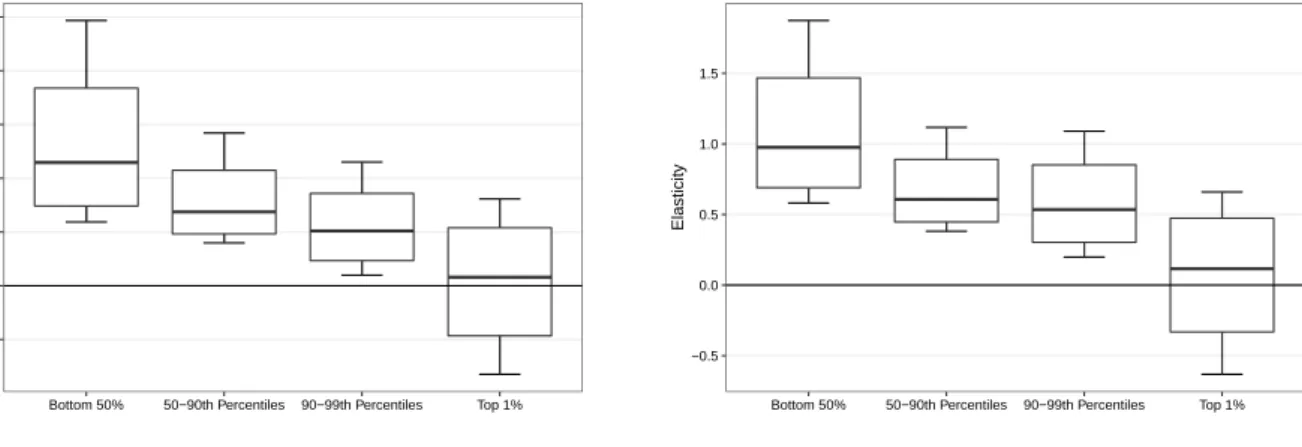
are key to understand household balance sheet dynamics across the wealth distribution. In particular, impulse responses suggest that the reaction of durable consumption is a decreasing function of net wealth. Variance decompositions assign a bulk of the variation found in con- sumption to the housing shock, especially for the bottom 50% of households. The historical decomposition shows that the cumulative effects of housing demand shocks have significantly affected consumption of the poorest during the Great Recession. However, we also find evidence that part of the cutback in top 1% consumption is explained by housing demand shocks in that period. Elasticities of consumption with respect to house prices, which are a byproduct of our structural model, suggest a larger spending sensitivity for weaker balance sheet households.
Our results are highly robust across both datasets.
The rest of the paper is organized as follows. Section 2 discusses the econometric framework and structural identification of the housing demand shock. The data are outlined in Section 3.
Impulse response functions and variance decompositions are analyzed in Section 4. Section 5 concludes. The Appendix provides additional results with alternative model specifications and gives a detailed overview of the data.
2 Econometric Framework
Structural macroeconomic shocks are often identified using small-scale VAR models in order to conserve degrees of freedom. The inclusion of only a couple of series, however, is likely to cause omitted variable problems that may affect impulse responses and variance decompositions alike (see Bernanke et al., 2005 for a thorough discussion). Moreover, economic concepts such as
”real activity” are hard to capture using only a specific data series. This issue is especially pronounced in the case considered here. Using only one or two housing series to identify a housing shock introduces an arguably large degree of arbitrariness. Finally, VARs allow to compute impulse responses only for the included variables, which is often a subset of what the researcher or policy-maker is interested about.
To take advantage of the information contained in large panel datasets we employ a dynamic factor model (seeStock and Watson,2016for an overview). Intuitively, the DFM approach boils down to extracting a small number of latent common factors that summarize the information from a much richer dataset. Consider the following dynamic factor model
yt=
s
X
l=0
λlft−l+et with et ∼iid.N(0, R) (1a)
ft=
h
X
p=1
φpft−p+t with t∼iid.N(0, Q) (1b) where yt is a (k×1) vector of observed variables and ft is a (m×1) vector of latent factors.
The number of factors is typically much smaller than the length of the cross-section, m << k.
The idiosyncratic disturbances et are uncorrelated at all leads and lags with ft and t and are assumed to have a diagonal covariance matrix R. The (k×m) loading matrices λl relate the factors to all economic and financial indicators. Note that if s > 0 then the factor lags are
allowed to directly affect the series in yt. Finally,φp are coefficient matrices, each of dimension (m×m), governing the dynamics in the state equation (1b). Clearly, the state equation follows the common VAR structure. The factor model can also be expressed in static form (see Stock and Watson, 2016) if we let h≥s+ 1, Ft = (ft0, . . . , ft−h+10 )0 and Λ∗ = (λ0, . . . , λs):
yt= ΛFt+et (2a)
Ft = ΦFt−1+ut (2b)
where Λ =
Λ∗ 0k×m(h−s−1)
, Φ = φ1 · · · φh
Im(h−1) 0m(h−1)×m
!
and ut= t 0m(h−1)×1
! .
Note that in contrast to studies using factor-augmented VAR (FAVAR) models, we do not impose that any factor be observed (for example, Bernanke et al. (2005) impose a short-term interest rate as observed factor and use this assumption for identificaton of the structural shock). For our purposes, it is also not necessary to provide an economic interpretation to the latent factors as inBelviso and Milani (2006).
2.1 Estimation
We rely on now standard Bayesian methods to estimate the model in (2a-2b). The likelihood- based approach is able to explicitly exploit the structure of the state equation in the estimation of the factors (see Bernanke et al., 2005). As a byproduct, it also delivers full posterior distri- butions naturally quantifying the extent of uncertainty. The estimation procedure consists of a multimove Gibbs sampler (Carter and Kohn,1994, see Kim and Nelson,1999 for an overview) in which the parameters are sampled conditional on the most recent draws of the factors, and the factors are drawn conditional on the most recent parameter estimates. Following Bai and Wang(2015), we employ the Jeffreys prior to account for the lack of a priori information about the model parameters. The Bayesian framework considered here is thus able to perform es- timation and inference of large dynamic factor models with a dynamic structure in both the observation and the state equation.
It is well known that due to indeterminacy the factor model is not identified without further restrictions (see Stock and Watson, 2016). The unobserved factors can always be rotated into an observationally equivalent representation. To achieve identification, we rely on the minimal restriction conditions derived inBai and Wang(2015). More exactly, we assume that the upper (m×m) block of λ0 is an identity matrix. Since the identifying restrictions concern only the contemporary loadings, the VAR(h) dynamics of the factors are left completely unrestricted. In other words, it is not necessary to impose the conventional practice that the covariance matrix of the dynamic factors ft is an identity matrix. A disturbance arising from the state equation is thus able to affect all macroeconomic and financial indicators in yt with no lags. The use of this minimal restriction strategy allows to impose contemporaneous sign restrictions on any series to identify our structural housing demand shock.
2.2 Structural Identification
We assume that the reduced-form vector of state-equation shocks t is a linear combination of structural shocks wt, such that t = A0wt. Under the assumption that E[wtwt0] = Im, we can decompose the covariance matrixQ=E[t0t] =E[A0wtwt0A00] =A0A00. One popular approach to fully identify the system is to chooseA0to be the Cholesky factor of the VAR covariance matrix as inSims (1980). It is well known that the triangular nature of the Cholesky factor implicitly imposes a temporal ordering (see, for example, the discussion in Canova and De Nicolo,2002).
In the context of housing shocks, this identification scheme has been followed by Cesa-Bianchi (2013) andBagliano and Morana(2012). In contrast,Buch et al.(2014),Cardarelli et al.(2009) and Jarocinski and Smets (2008) impose a mixture of sign and zero restrictions, assuming that output or prices react to housing shocks only with a lag. Given the many channels through which the housing market may affect the economy, such zero restrictions are arguably imposing strong identifying assumptions. For that reason, we adopt the agnostic identification strategy by Uhlig (2005) and, for the factor model framework, Ahmadi and Uhlig (2015), and only re- strict the sign of selected variables.
All sign restrictions are theoretically motivated and are keeping with a large literature summa- rized in Justiniano et al. (2015), Christiano et al. (2014) and Furlanetto et al. (2019). More specifically, we identify the housing demand shock by imposing that real GDP, core prices of personal consumption expenditures (PCE) and the three month treasury bill rate react posi- tively upon impact. This rules out that the identified shock is contaminated with supply or monetary shocks. It is, however, more challenging to disentangle the housing demand shock from investment shocks (see Justiniano et al., 2010) and other demand shocks (for example discount factor or fiscal shocks). Our strategy follows Furlanetto et al. (2019), who suggest that traditional demand shocks can be excluded by imposing a positive sign restriction on the response of the ratio of (real gross private domestic) investment over output.1 Investment and housing shocks are thus assumed to create investment booms. To further separate housing from investment shocks we restrict stock prices as measured by the S&P 500 to react positively.2 Note that up to now, it is still not possible to distinguish a positive housing shock from a shock originating in the credit markets. Keeping with Furlanetto et al. (2019) and the literature in Justiniano et al. (2015), we restrict the loan-to-value (LTV) ratio to react negatively. This allows total credit to increase under the restriction that the value of real estate does so by more.3 Finally, a positive housing demand shock increases real estate loans as well as quantity and prices of housing (Iacoviello and Neri,2010). We therefore use our detailed dataset to im- pose positive sign restrictions on aggregate real estate loans as well as on building permits and house prices in all four Census regions4. Since a shock is unexpected by nature, it is arguably more appropriate to constrain permits instead of housing starts, which are left unrestricted. In contrast to small-scale VAR studies also using sign restrictions (Andr´e et al., 2012, Furlanetto
1Restricting the ratio allows investment to increase when faced with a demand shock but less so than the remaining part of aggregate demand.
2A positive investment shock increases the supply of capital and lowers its price. Since the price of capital is taken as a proxy of the stock market value for firms, an investment shock negatively impacts the value of equity (see the discussion inFurlanetto et al.,2019andChristiano et al.,2014).
3More exactly, total credit amounts to total loans to the non-financial private sector, while housing value is given by real estate at market value of households and non-profit organisations.
4The US Census Bureau splits the U.S. into four regions: the Northeast, the Midwest, the South, and the West.
et al.,2019), our factor model allows testing whether the identified housing shock actually leads to new housing units being built.
To incorporate the sign restrictions we employ the procedure described in Rubio-Ramirez et al. (2010). For each draw from the reduced-form posterior, the algorithm works as fol- lows. First, we produce Achol0 using the Cholesky decomposition of the covariance matrix Q to obtain uncorrelated shocks as in a recursively identified model. Then we compute the QR decomposition ofW =QR, whereW is a (m×m) matrix filled with independent standard nor- mally distributed variables. Post-multiplying Achol0 by Q forms a candidate structural impact matrix Acand0 = Achol0 Q. Contemporaneous impulse responses are then generated according to yirf0 = Λ∗Acand0 , which allows to check the sign restrictions. If this is not the case we draw a new W and repeat the procedure until the sign restrictions are satisfied. Note that we follow the recommendations of Canova and Paustian (2011) in two ways. First, we restrict only impact responses to avoid the often questionable dynamic constraints. Second, the factor model frame- work allows us to impose a large number of sign restrictions to identify the structural shock.
Moreover, all sign restrictions are motivated by the dynamic stochastic general equilibrium (DSGE) literature as advised byMusso et al. (2011).
3 Data
We estimate the dynamic factor model on two quarterly datasets, one containing 73 and the other 160 indicators. As suggested by Bai and Ng(2008a) and Boivin and Ng (2006), a larger cross-section may not necessarily improve estimation accuracy in factor models. It thus seems appropriate to use both a relatively small dataset consisting of only key series and a large one to check the robustness of the results. The sample starts in 1989Q3 and ends in 2019Q3. All indicators are transformed to induce stationarity, see the Appendix for a detailed description.
The large dataset is an augmented version of the FRED-QD database (seeMcCracken and Ng, 2020) with the main difference that household balance sheet data has been added. The smaller dataset builds on the same database but focuses on key economic indicators, the housing and credit market and household balance sheet data.
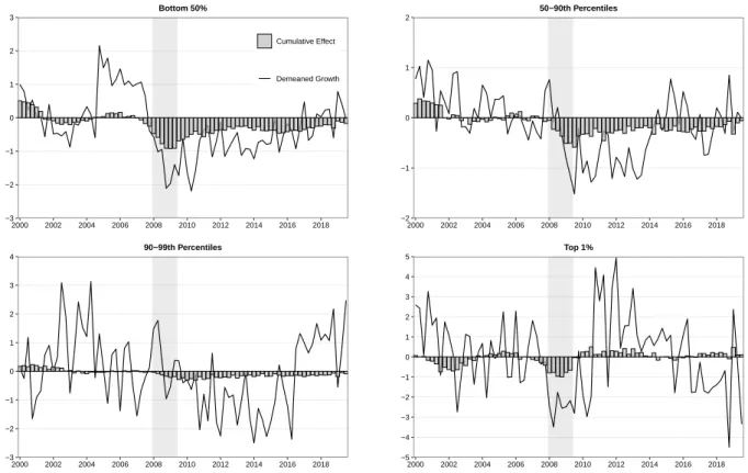
To evaluate whether a housing demand shock has heterogeneous effects on households’ bal- ance sheets we draw on the Distributional Financial Accounts (DFAs) provided by the Board of Governors (see Batty et al., 2019). The relatively new DFAs contain detailed time series on the assets and liabilities held by four different wealth percentile groups (bottom 50%, 50th to 90th percentiles, 90th to 99th percentiles, and the top 1%). Figure 1 shows the evolution of real net wealth for all wealth percentile groups. The greatest wealth losses are found between 2007Q3 and 2009Q1 and are especially concentrated on households belonging to the top decile.
The subsequent recovery is associated with an unprecedented wealth level, however unequally distributed among the population. While net worth of the bottom 50% is close to zero for the entire sample, the top 1% accounts for a substantial fraction of U.S. wealth. In 2019Q3, around 70% of wealth is held by the top decile. The heterogeneous evolution among wealth groups is clearly related to individual composition effects. Wealthier households have traditionally been
0 20 40 60 80 100
1990 1992 1994 1996 1998 2000 2002 2004 2006 2008 2010 2012 2014 2016 2018 2020
Trillions of nominal dollars
Top 1%
90−99th Percentiles 50−90th Percentiles Bottom 50%
Figure 1: Evolution of Net Worth
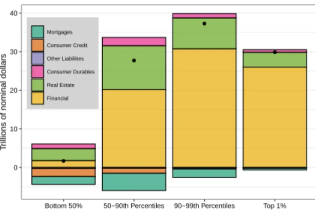
0 10 20 30 40
Bottom 50% 50−90th Percentiles 90−99th Percentiles Top 1%
Trillions of nominal dollars
Mortgages Consumer Credit Other Liabilities Consumer Durables Real Estate Financial
Figure 2: Balance Sheet Composition 2019Q3
exposed more to cyclical assets like equity, as the largest fraction of wealth is of financial nature (see Figure 2 for 2019Q3). Real estate is the principal asset component for households belong- ing to the bottom 50%. In contrast to other percentile groups, financial assets account for only a minor share of total assets. The liability side shows the poorest households’ dependence on consumer credit, as they hold over half of total consumer credit.
In order to ensure that results are not driven by population differences from the different- sized wealth groups, we scale the series of each group by the respective number of percentiles.5 Moreover, all series enter the estimation procedure in standardized form.
4 Results
In this section, we present empirical results from our dynamic factor model with both datasets.
To determine the number of unobserved factors, m, we compute the information criteria ICp2
and BIC3 by Bai and Ng (2002) (see also the discussion in Bai and Ng, 2008b), the ER and GR criteria by Ahn and Horenstein (2013) and the IC1,c,nT∗ and IC2,c,nT∗ criteria by Alessi et al.
(2010). For the smaller dataset, all criteria suggest five factors except forER = 2 andICp2 = 8.
The same two criteria are estimated to be ER = 2 and ICp2 = 6 with the rich dataset, while all other suggest four factors. We follow the majority and setm= 5 for the narrow and m= 4 for the more extensive database, but report results for a range of alternative specifications in the Appendix. We sets= 1 in observation equation (1a), thus allowing a dynamic relationship between the latent states and the variables. According to the Bayesian information criterion (BIC), the factor dynamics in (1b) are characterized by a VAR(1) for the smaller and a VAR(2) for the larger dataset. We follow Uhlig (2005) and report the pointwise median together with 68% posterior bands. The yt vector has been ordered such that the first m series are given by leading indicators of different data groups.6 All results are based on 90’000 draws from the Gibbs sampler, from which the first 87’000 are discarded as burn-in.
The presentation of our empirical results is organized around our two research questions. We
5For example, credit held by the bottom 50% is divided by 50.
6More specifically, the first five series consist of real GDP, the industrial production index, the total number of nonfarm employees, total housing starts, and the S&P 500. See the Appendix for a detailed list of the groups and series. Random permutations of the observation vector had negligible effects on our results.
begin with the question of how the housing demand shock is transmitted to the aggregate US economy before analyzing the responses of households’ balance sheets.
4.1 How Are Housing Demand Shocks Transmitted to the Aggregate Economy?
4.1.1 Impulse Responses
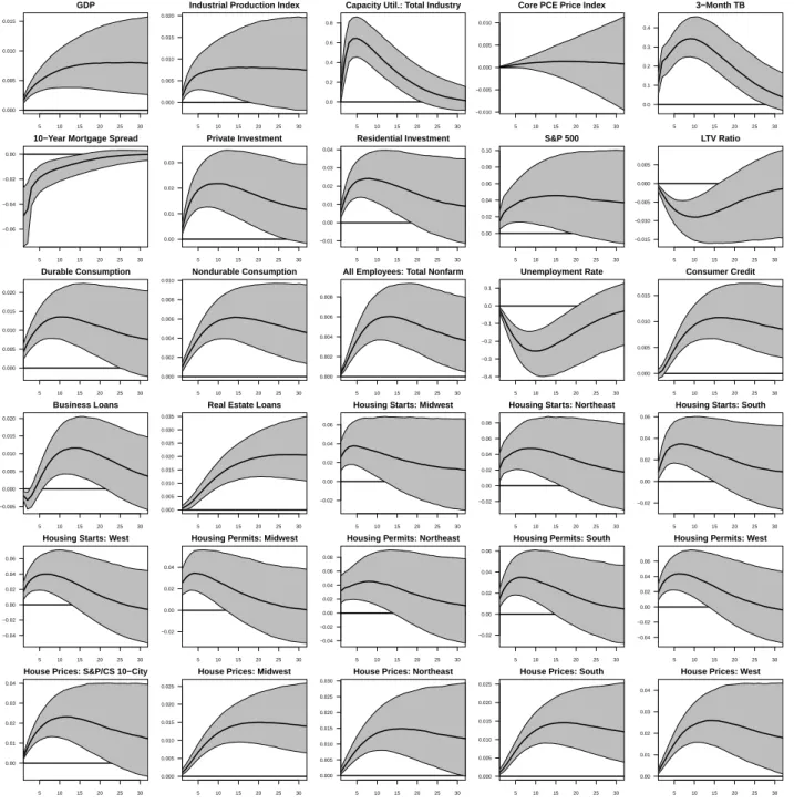
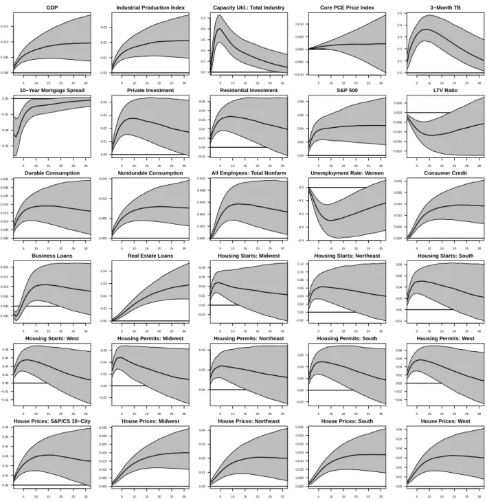
Figure 3 plots the impulse responses, estimated on the smaller sample, of the level of key indicators to a one standard deviation housing demand shock. The black line reports the median response. Results from the large dataset are vastly similar and therefore relegated to the Appendix (see figure 8).
5 10 15 20 25 30
0.000 0.005 0.010 0.015
GDP
5 10 15 20 25 30
0.000 0.005 0.010 0.015 0.020
Industrial Production Index
5 10 15 20 25 30
0.0 0.2 0.4 0.6 0.8
Capacity Util.: Total Industry
5 10 15 20 25 30
−0.010
−0.005 0.000 0.005 0.010
Core PCE Price Index
5 10 15 20 25 30
0.0 0.1 0.2 0.3 0.4
3−Month TB
5 10 15 20 25 30
−0.06
−0.04
−0.02 0.00
10−Year Mortgage Spread
5 10 15 20 25 30
0.00 0.01 0.02 0.03
Private Investment
5 10 15 20 25 30
−0.01 0.00 0.01 0.02 0.03 0.04
Residential Investment
5 10 15 20 25 30
0.00 0.02 0.04 0.06 0.08 0.10
S&P 500
5 10 15 20 25 30
−0.015
−0.010
−0.005 0.000 0.005
LTV Ratio
5 10 15 20 25 30
0.000 0.005 0.010 0.015 0.020
Durable Consumption
5 10 15 20 25 30
0.000 0.002 0.004 0.006 0.008 0.010
Nondurable Consumption
5 10 15 20 25 30
0.000 0.002 0.004 0.006 0.008
All Employees: Total Nonfarm
5 10 15 20 25 30
−0.4
−0.3
−0.2
−0.1 0.0 0.1
Unemployment Rate
5 10 15 20 25 30
0.000 0.005 0.010 0.015
Consumer Credit
5 10 15 20 25 30
−0.005 0.000 0.005 0.010 0.015 0.020
Business Loans
5 10 15 20 25 30
0.000 0.005 0.010 0.015 0.020 0.025 0.030 0.035
Real Estate Loans
5 10 15 20 25 30
−0.02 0.00 0.02 0.04 0.06
Housing Starts: Midwest
5 10 15 20 25 30
−0.02 0.00 0.02 0.04 0.06 0.08
Housing Starts: Northeast
5 10 15 20 25 30
−0.02 0.00 0.02 0.04 0.06
Housing Starts: South
5 10 15 20 25 30
−0.04
−0.02 0.00 0.02 0.04 0.06
Housing Starts: West
5 10 15 20 25 30
−0.02 0.00 0.02 0.04
Housing Permits: Midwest
5 10 15 20 25 30
−0.04
−0.02 0.00 0.02 0.04 0.06 0.08
Housing Permits: Northeast
5 10 15 20 25 30
−0.02 0.00 0.02 0.04 0.06
Housing Permits: South
5 10 15 20 25 30
−0.04
−0.02 0.00 0.02 0.04 0.06
Housing Permits: West
5 10 15 20 25 30
0.00 0.01 0.02 0.03 0.04
House Prices: S&P/CS 10−City
5 10 15 20 25 30
0.000 0.005 0.010 0.015 0.020 0.025
House Prices: Midwest
5 10 15 20 25 30
0.000 0.005 0.010 0.015 0.020 0.025 0.030
House Prices: Northeast
5 10 15 20 25 30
0.000 0.005 0.010 0.015 0.020 0.025
House Prices: South
5 10 15 20 25 30
0.00 0.01 0.02 0.03 0.04
House Prices: West
Figure 3: Dynamic responses of variables to housing demand shock using the small dataset Notes: The figure plots the impulse responses of the level of key variables to the identified housing demand shock. The gray areas indicate the 68% posterior probability regions. The straight black line indicates the posterior median at each horizon.
In line with the transmission channels discussed above, a housing demand shock generates a significant and persistent economic boom. Real GDP, industrial production, and capacity uti- lization increase between 0.5 and 0.6% within one year. Residential investment, a subcomponent of GDP measuring the purchase of newly built residential structures, rises disproportionally by 2% after four quarters. The economic expansion is reflected in the labour market indicators, as the unemployment rate decreases while the total number of nonfarm employees grows. On the credit side, real estate loans and consumer credit increase persistently over the impulse horizon, which conforms to the collateral channel of a housing demand shock. The fact that business loans grow only slightly and return to their initial level stands in contrast to studies identifying credit shocks (for example, Boivin et al., 2018), thus pointing towards a successful disentan- glement of credit and housing shocks. The LTV ratio is restricted to be negative on impact but stays so for at least four years. Conforming to consumption smoothing arguments from life-cycle models, both durable and nondurable consumption rise. Importantly, the response of durable consumption is more pronounced in magnitude than for nondurable consumption.
Financial variables mirror the boom of real economic indicators. The 3-month treasury bill rate is hump-shaped, suggesting that the Fed increases its benchmark rate as a reaction to the initial rise of GDP growth and the capacity utilization index. The median response of the S&P 500 stock market index increases by around 4% over the horizon. Interestingly, the reaction of the consumption price index is relatively muted despite the economic expansion, confirming the empirical results in Furlanetto et al. (2019). More exactly, the core PCE price index is slightly positive for only a few quarters, after which the posterior distribution centers around the zero line. In contrast, house price indices of all four Census regions react strongly positive to the housing demand shock over the entire horizon. The S&P/Case-Shiller 10-City home price index, which was left unrestricted also on impact, confirms the price hike. In line with Tobin’s q effect, rising prices for housing are associated with a general increase of building permits for at least three years. The fact that the unrestricted housing starts rise in all four geographic areas provides further comfort to our identifying assumptions.
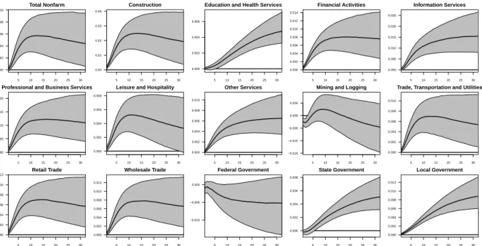
All impulse responses discussed are robust to the choice of the dataset, even though the model specification differs and the extensive dataset contains more than twice as much variables as the smaller one.7 Among these additional series are sectoral employment indicators, which provide further evidence that a housing shock has in fact been identified. Figure 9 in the Appendix plots the respective impulse responses and shows that the construction sector features the most pronounced reaction among all sectors.
4.1.2 Variance Decompositions
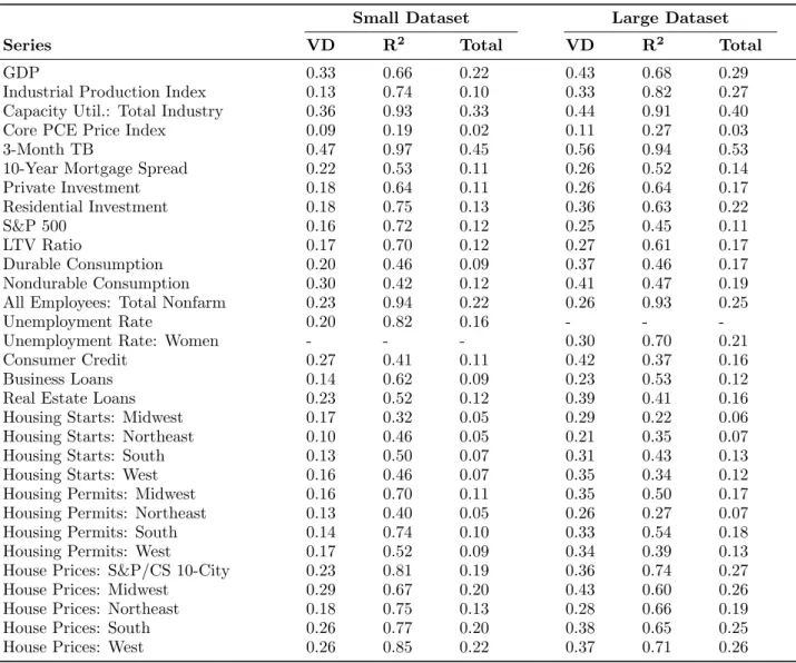
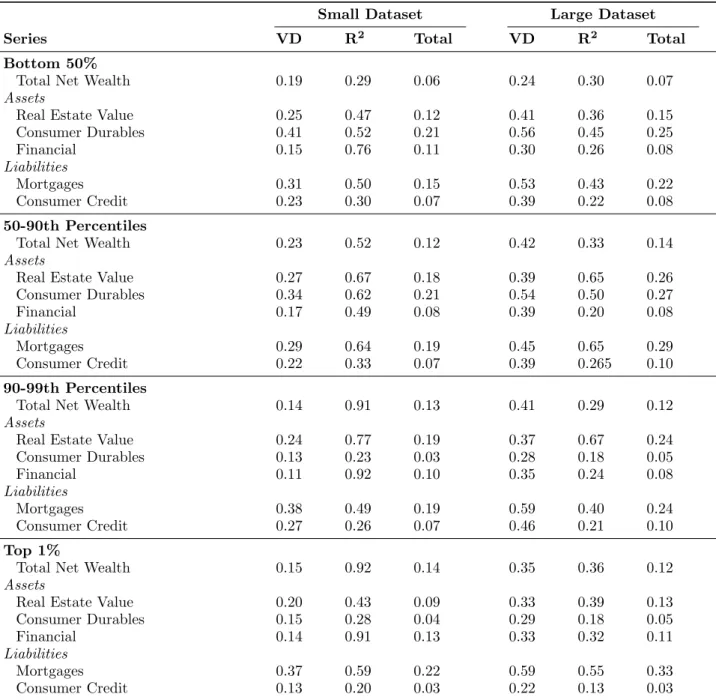
Table 1 shows the importance of housing demand shocks in explaining economic fluctuations during our 1989-2019 sample. While variance decompositions are calculated for each draw that satisfies the sign restrictions, the table presents median values at a 32-quarter horizon. The second column reports the fraction of the common component of the series explained by the housing demand shock. The third column shows the contribution of the common component to the overall variance of the indicators. The fourth column is simply the product of the previous
7Further robustness tests are reported in Appendix figures11and12, covering a wide range of alternative model specifications.
two and represents the fraction of the total variability explained by the housing demand shock.
The next three columns show the results for the large dataset.
In line with the literature, our variance decompositions show that housing demand shocks are significant drivers of business cycle fluctuations. The housing shock explains between 24 and 44% of the variance of the common component of real economic indicators such as GDP, the industrial production index and the capacity utilization measure. Labor market indicators, credit series and the 3-month TB rate are also well explained. Importantly, the housing demand shock has high explanatory power for housing starts, housing permits and house price variation for all four Census regions. Column four and seven indicate that our structural model explains around 20% of total variation in house price series. Column three and six of Table 1 show that five and four unobserved factors are able to capture a large fraction of fluctuations in key economic indicators.
Table 1: Variance Decompositions andR2
Small Dataset Large Dataset
Series VD R2 Total VD R2 Total
GDP 0.33 0.66 0.22 0.43 0.68 0.29
Industrial Production Index 0.13 0.74 0.10 0.33 0.82 0.27
Capacity Util.: Total Industry 0.36 0.93 0.33 0.44 0.91 0.40
Core PCE Price Index 0.09 0.19 0.02 0.11 0.27 0.03
3-Month TB 0.47 0.97 0.45 0.56 0.94 0.53
10-Year Mortgage Spread 0.22 0.53 0.11 0.26 0.52 0.14
Private Investment 0.18 0.64 0.11 0.26 0.64 0.17
Residential Investment 0.18 0.75 0.13 0.36 0.63 0.22
S&P 500 0.16 0.72 0.12 0.25 0.45 0.11
LTV Ratio 0.17 0.70 0.12 0.27 0.61 0.17
Durable Consumption 0.20 0.46 0.09 0.37 0.46 0.17
Nondurable Consumption 0.30 0.42 0.12 0.41 0.47 0.19
All Employees: Total Nonfarm 0.23 0.94 0.22 0.26 0.93 0.25
Unemployment Rate 0.20 0.82 0.16 - - -
Unemployment Rate: Women - - - 0.30 0.70 0.21
Consumer Credit 0.27 0.41 0.11 0.42 0.37 0.16
Business Loans 0.14 0.62 0.09 0.23 0.53 0.12
Real Estate Loans 0.23 0.52 0.12 0.39 0.41 0.16
Housing Starts: Midwest 0.17 0.32 0.05 0.29 0.22 0.06
Housing Starts: Northeast 0.10 0.46 0.05 0.21 0.35 0.07
Housing Starts: South 0.13 0.50 0.07 0.31 0.43 0.13
Housing Starts: West 0.16 0.46 0.07 0.35 0.34 0.12
Housing Permits: Midwest 0.16 0.70 0.11 0.35 0.50 0.17
Housing Permits: Northeast 0.13 0.40 0.05 0.26 0.27 0.07
Housing Permits: South 0.14 0.74 0.10 0.33 0.54 0.18
Housing Permits: West 0.17 0.52 0.09 0.34 0.39 0.13
House Prices: S&P/CS 10-City 0.23 0.81 0.19 0.36 0.74 0.27
House Prices: Midwest 0.29 0.67 0.20 0.43 0.60 0.26
House Prices: Northeast 0.18 0.75 0.13 0.28 0.66 0.19
House Prices: South 0.26 0.77 0.20 0.38 0.65 0.25
House Prices: West 0.26 0.85 0.22 0.37 0.71 0.26
Notes: The second column reports the fraction of the common component of the series explained by the housing demand shock at a 32-quarter horizon. The third column shows the contribution of the common component to the overall variance of the indicators. The fourth column is simply the product of the previous two and represents the fraction of the total variability explained by the housing demand shock. The next three columns show the results for the large dataset.
4.2 Do Households Respond Differently to the Housing Demand Shock Depending on Net Wealth?
The substantial aggregate effects of a housing demand shock demonstrate the importance of understanding the underlying transmission channels. Of particular interest after the financial crisis has been the relationship between fluctuations in housing wealth and the response of consumption. In fact, housing market spillovers are suggested to be largely concentrated on consumption (Iacoviello and Neri,2010). As outlined above, an increase of housing wealth may a) raise collateral and therefore mitigate credit constraints and b) increase consumption due to the wealth effect. Both channels are arguably sensitive to the cross-sectional distribution of wealth and the composition of households’ balance sheets. For example, richer households are less likely to face credit constraints and may give the precautionary savings motive a small role.
This translates into a smaller elasticity to consume out of wealth compared to the poor. As a consequence, the aggregate consequences of a housing shock might largely be driven by the consumption response of poorer households, although housing is a substantial balance sheet component for all wealth percentile groups.
Given the economic importance, an extensive number of studies have analyzed whether and to what extent (housing) wealth shocks cause heterogeneous responses among households. The hypothesis of a representative agent is typically rejected and economically significant wealth ef- fects are reported (see, for example,Mian and Sufi,2011,Mian et al.,2013,Guren et al.,2020b, Aladangady, 2017, Berger et al., 2017). To isolate the housing wealth effect, empirical studies frequently rely on cross-regional regressions using exogeneous sources of housing variation as instruments. This strategy delivers partial equilibrium estimates, as aggregate general equilib- rium effects are absorbed by the constant or the time fixed effect in a panel regression.8 In contrast and highly complementary to this strand of literature, we are interested in the general equilibrium effects of housing shocks. Looking again at the consumption response of different wealth percentile groups, it is interesting to see whether the implications of partial equilibrium estimates still hold. For example, it is well possible that the financial wealth effect associated with booming stock markets ignites consumption of the rich, thus leveling the cross-sectional consumption response. To understand the aggregate general equilibrium dynamics in the last section we thus analyze the general equilibrium behavior of households’ balance sheets. In con- trast to studies using DSGE models (Berger et al., 2017, Guren et al., 2020b, among others), our DFM imposes little structure a priori, thus mitigating the possibility that results are driven by a potentially misspecified model structure. Clearly, this comes at the cost of not being able to obtain ”deep” structural parameters, for example the wealth effect of housing values con- ditional on household characteristics. It is also important to note a drawback concerning the disaggregated consumption measures used in this study. The use of household balance sheet data implies that nondurable consumption is not available, so that only the reaction of durable consumption can be estimated. However, comparing both aggregate consumption responses in the last section shows a relatively muted reaction for nondurable consumption in terms of magnitude. Durable consumption and (residential) investment are the primary forces driv-
8AsGuren et al.(2020a) point out, the clear theoretical interpretation of cross-regional partial equilibrium estimates might be contaminated by local general equilibrium effects. They suggest to divide cross-regional estimates by an estimate of the local fiscal multiplier to adjust for local general equilibrium effects.
ing the pronounced GDP response. The literature also suggests that increased spending due to housing wealth is largely concentrated on durable goods (Mian et al., 2013, Andersen and Leth-Petersen, 2019).
4.2.1 Impulse Responses
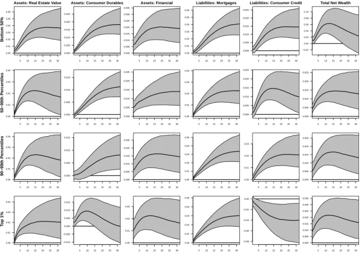
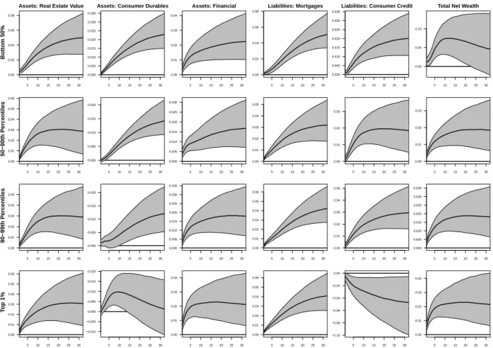
Estimated on the small sample, figure 4 plots impulse responses of the level of real household balance sheet components to the housing demand shock. The first five columns show assets and liabilities, while the last column plots the response of total net wealth. Rows list the four wealth percentile groups. Results from the large dataset are almost identical,9 see Appendix figure 10. Note that responses are highly data-driven, as all balance sheet series are left completely unrestricted.
5 10 15 20 25 30
0.00 0.01 0.02 0.03 0.04 0.05 0.06
Assets: Real Estate Value
5 10 15 20 25 30
0.000 0.005 0.010 0.015 0.020 0.025
Assets: Consumer Durables
5 10 15 20 25 30
0.000 0.005 0.010 0.015 0.020 0.025 0.030 0.035
Assets: Financial
5 10 15 20 25 30
0.00 0.01 0.02 0.03 0.04 0.05 0.06
Liabilities: Mortgages
5 10 15 20 25 30
0.000 0.005 0.010 0.015 0.020 0.025
Liabilities: Consumer Credit
5 10 15 20 25 30
−0.02 0.00 0.02 0.04 0.06 0.08 0.10
Total Net Wealth
5 10 15 20 25 30
0.00 0.01 0.02 0.03 0.04
5 10 15 20 25 30
0.000 0.005 0.010 0.015
5 10 15 20 25 30
0.000 0.005 0.010 0.015 0.020 0.025
5 10 15 20 25 30
0.00 0.01 0.02 0.03 0.04
5 10 15 20 25 30
0.000 0.005 0.010 0.015 0.020 0.025
5 10 15 20 25 30
0.000 0.005 0.010 0.015 0.020 0.025
5 10 15 20 25 30
0.00 0.01 0.02 0.03 0.04
5 10 15 20 25 30
0.000 0.005 0.010 0.015
5 10 15 20 25 30
0.000 0.005 0.010 0.015 0.020 0.025
5 10 15 20 25 30
0.00 0.01 0.02 0.03 0.04 0.05
5 10 15 20 25 30
0.00 0.01 0.02 0.03
5 10 15 20 25 30
0.000 0.005 0.010 0.015 0.020 0.025
5 10 15 20 25 30
0.00 0.01 0.02 0.03 0.04
5 10 15 20 25 30
−0.010
−0.005 0.000 0.005 0.010 0.015
5 10 15 20 25 30
0.00 0.01 0.02 0.03
5 10 15 20 25 30
0.00 0.01 0.02 0.03 0.04 0.05
5 10 15 20 25 30
−0.08
−0.06
−0.04
−0.02 0.00
5 10 15 20 25 30
0.000 0.005 0.010 0.015 0.020 0.025 0.030 0.035
Bottom 50%50−90th Percentiles90−99th PercentilesTop 1%
Figure 4: Dynamic responses of household balance sheet variables to housing demand shock using the small dataset
Notes: The figure plots the impulse responses of the level of households’ balance sheet components to the identified housing demand shock. The gray areas indicate the 68% posterior probability regions. The straight black line indicates the posterior median at each horizon.
A quick glance is enough to observe that a housing demand shock is associated with a general expansion of balance sheets across all wealth segments. The increase of assets generally dom- inates the higher debt burden, although net wealth for households belonging to the bottom 50% slowly revert to the initial state. All groups participate in the newly built structures,
9Most impulse responses are slightly more pronounced with the large dataset. Appendix figures13and14confirm the benchmark results for a wide range of alternative model specifications.