How Important Are Uncertainty Shocks in the Housing Market?

How Important Are Uncertainty Shocks in the Housing Market?

Johannes Strobel

September 29, 2016

How Important Are Uncertainty Shocks in the Housing Market?

A dissertation submitted to the graduate faculty in partial fulfillment of the requirements for the degree of Doktor der Wirtschaftswissenschaft (Dr. rer. pol.).

Advisors:

Prof. Gabriel Lee Prof. Kevin Salyer

Wirtschaftswissenschaftliche Fakult¨ at Universit¨ at Regensburg

Regensburg, Germany

Acknowledgement

I can not be sufficiently grateful for the guidance, advice and support from Prof. Gabriel Lee.

I am also indebted to Prof. Kevin Salyer for his support and advice. Moreover, I would like

to thank Victor Dorofeenko, Georg Lindner, Binh Nguyen-Thanh, Martina Weber and Kerstin

Zeise. For financial support, I thank the German Research Society (Deutsche Forschungsge-

meinschaft) and the Bavarian Graduate Program in Economics. Finally, I am grateful to my

family for their outstanding support.

Contents

1 Introduction 1

2 On Measuring Uncertainty Shocks 4

2.1 Introduction . . . . 4

2.2 Data . . . . 5

2.3 Results . . . . 6

2.4 Conclusion . . . . 9

2.5 Appendix . . . . 9

3 Hump-shape Uncertainty, Agency Costs and Aggregate Fluctuations 11 3.1 Introduction . . . . 11

3.2 Motivation . . . . 13

3.3 Model . . . . 15

3.4 GHH Preferences and Variable Capital Utilization . . . . 25

3.5 Conclusion . . . . 31

3.6 Appendix . . . . 32

4 Housing and Macroeconomy: The Role of Credit Channel, Risk -, Demand - and Monetary Shocks 36 4.1 Introduction . . . . 36

4.2 Model: Housing Markets, Financial Intermediation, and Monetary Policy . . . . 40

4.3 Empirical Results . . . . 60

4.4 Some Final Remarks . . . . 72

4.5 Appendix . . . . 74

5 Conclusion 83

6 Bibliography 85

List of Figures

2.1 IQR, standard deviation and uncertainty proxy for the manufacturing sector, the services sector and the U.S. economy using profit growth. . . . 7 2.2 IQR, standard deviation and uncertainty proxy for the manufacturing sector, the

services sector and the U.S. economy using stock returns. . . . 8 3.1 Financial Uncertainty and Macro Uncertainty measures from 1960 to 2015. . . . 13 3.2 Impulse Response Functions of the VAR. . . . . 15 3.3 The partial equilibrium impact of an uncertainty shock. . . . 18 3.4 Modeling Uncertainty Shocks using different persistence parameters. . . . 19 3.5 Impulse responses of output, household consumption and investment following an

uncertainty shock for persistence parameters. . . . 22 3.6 Impulse responses of the risk premium, the bankruptcy rate, return to invest-

ment and the relative price of capital following an uncertainty shock for different persistence parameters. . . . . 23 3.7 Impulse responses of output, consumption and investment following an uncer-

tainty shock for different magnitudes of monitoring costs. . . . 24 3.8 Impulse responses of output, household consumption and investment following a

shock (jump and hump) to uncertainty. . . . . 27 3.9 Lending channel variables following a shock (jump and hump) to uncertainty. . . 28 4.1 Real housing prices for the U.S. and selected European countries from 1997 until

2007. . . . 37

4.2 Implied flows for the economy. . . . . 41

4.3 Estimated productivity and risk shocks from 2001 until 2011. . . . 65

4.4 Impulse response of GDP, Total Capital and Consumption (PCE) to a 1% increase

in Uncertainty; LTV = 0.1. . . . 67

4.5 Impulse response of GDP, Total Capital and Consumption (PCE) to a 1% increase in Uncertainty; LTV = 0.85. . . . 68

4.6 Impulse response of Housing Markup, Risk Premium on Loans, and Bankruptcy Rate to a 1% increase in Uncertainty; LTV = 0.1. . . . . 69

4.7 Impulse response of Housing Markup, Risk Premium on Loans, and Bankruptcy Rate to a 1% increase in Uncertainty; LTV = 0.85. . . . 70

4.8 Impulse response of Land Price, Housing Price and Borrowing amount to a 1% increase in Uncertainty; LTV = 0.1. . . . . 71

4.9 Impulse response of Land Price, Housing Price and Borrowing amount to a 1% increase in Uncertainty; LTV = 0.85. . . . 72

4.10 Annual residential investment from 1997 until 2011. . . . . 74

4.11 Household Debt: Long Term Loan for House Purchase. . . . 75

4.12 Lending Rates (> 5 years) for House Purchases. . . . 76

List of Tables

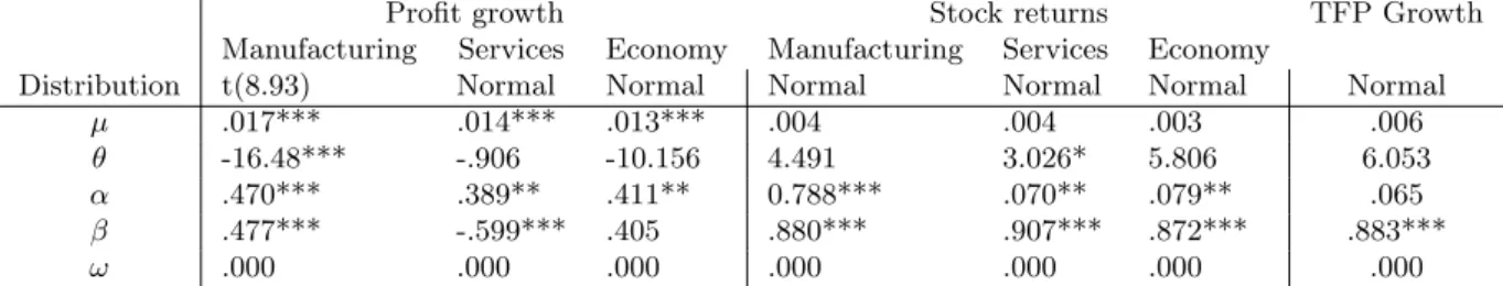
2.1 Parameter estimates of the GARCH-M model. . . . . 6

2.2 Correlation coefficients of uncertainty proxies. . . . 8

2.3 LM test results. . . . 9

2.4 Summary statistics of the Uncertainty Measures. . . . 10

2.5 Standardized residuals after GARCH-M estimation . . . . 10

3.1 Benchmark calibration for the monthly frequency. . . . 21

3.2 Correlation coefficients of consumption, investment, bankruptcy rate and uncer- tainty with output. . . . 25

3.3 Benchmark calibration for the monthly frequency with GHH preferences and vari- able capital utilization. . . . 26

3.4 Business Cycle Characteristics. . . . 29

3.5 Variance Decomposition: Hump-shaped uncertainty shocks, TFP shocks and the coefficient of relative risk aversion. . . . 29

3.6 Variance Decomposition: TFP shocks, uncertainty shocks and the agency friction. 30 4.1 Key Preference, Lending and Production Parameters. . . . . 61

4.2 Intermediate Production Technology Parameters. . . . 62

4.3 Variance Decomposition of Forecast Error. . . . 73

4.4 Interest rate type, loan term and lenders across countries. . . . 77

4.5 Loan to Value Ratios for selected countries. . . . 78

Chapter 1

Introduction

This dissertation analyzes the impact of shocks to uncertainty on the macroeconomy and on the housing sector. To this end, I examine different approaches to measuring and modeling uncertainty. My work contributes to this growing literature as follows. Chapter two clarifies one possible source of confusion in the calibration of models using uncertainty shocks, that between ex-ante vs. ex-post uncertainty measures. Chapter three proposes a different approach to modeling uncertainty shocks, that corresponds to the empirical evidence of Jurado, Ludvigson and Ng (2015) and Ludvigson, Ma, and Ng (2016). Chapter four investigates how the factors of production uncertainty, financial intermediation, and credit constrained households can affect housing prices and aggregate economic activity.

Uncertainty as a factor influencing or governing decisions of economic agents has experienced

increasing attention in recent years. Early work, such as Bernanke (1983) and McDonald and

Siegel (1986), assumes irreversibility of investments to generate real options effects. More recent

work, such as Dorofeenko, Lee, and Salyer (2008, 2014) or Christiano, Motto and Rostagno

(2014), focuses on the impact of uncertainty in the context of financial frictions in Dynamic

Stochastic General Equilibrium models. In these models, productivity’s time-varying second

moment is part of the policy function despite first order approximation and impacts an economy

via the optimal contract between borrowers and lenders. The literature on uncertainty and

macroeconomics is divided, however, on the (magnitude of the) effects and the propagation

mechanism of uncertainty on aggregate fluctuations. Dorofeenko et al. (2008), for instance,

examine a 1% unexpected jump in uncertainty and find a large impact on the credit channel

but little impact on real variables. Dorofeenko et al. (2014), which combines the model of

Dorofeenko et al. (2008) with the multi-sector model of Davis and Heathcote (2005) to examine

the impact of risk on the housing market, show that uncertainty matters for the housing market and especially for housing prices - but not so much for real variables. Christiano et al. (2014), in contrast, add a news component to uncertainty shocks and report that risk shocks are the most important source of business cycle fluctuations. As virtually all the work is done by the exogenous definition of the exogenous risk shocks, as shown by Lee, Salyer and Strobel (2016), it is crucially important to properly model and calibrate uncertainty. To this end, various proxies have been proposed in the literature.

Chapter two

¹

, On Measuring Uncertainty Shocks, empirically shows systematic differences in those proxies, as realized variables fluctuate more than the measures that are based on forecasts.

More precisely, the variation in the realized cross-sectional standard deviation of profit growth and stock returns is larger than the variation in the forecast standard deviation.

Chapter three

²

, Hump-shape Uncertainty, Agency Costs and Aggregate Fluctuations, intro- duces a different approach to modeling uncertainty shocks. The uncertainty measures due to Jurado, Ludvigson and Ng (2015) and Ludvigson, Ma, and Ng (2016) show a hump-shape time path: Uncertainty rises for two years before its decline. Current literature on the effects of uncertainty on macroeconomics, including housing, has not accounted for this observation. This chapter shows that when uncertainty rises and falls over time, then the output displays hump- shape with short expansions that are followed by longer and persistent contractions. And because of these longer and persistent contractions in output, uncertainty is, on average, counter-cyclical.

The model builds on the literature combining uncertainty and financial constraints. We model the time path of uncertainty shocks to match empirical evidence in terms of shape, duration and magnitude. In the calibrated models, agents anticipate this hump-shape uncertainty time path once a shock has occurred. Thereby, agents respond immediately by increasing invest- ment (i.e. pre-cautionary savings), but face a substantial drop in investment, consumption and output as more uncertain times lie ahead. With persistent uncertain periods, both risk premia and bankruptcies increase, which cause a further deterioration in investment opportunities. Be- sides, accounting for hump-shape uncertainty measures can result in a large quantitative effect of uncertainty shock relative to previous literature.

Chapter four

³

, Housing and Macroeconomy: The Role of Credit Channel, Risk -, Demand - and Monetary Shocks, uses the standard approach to modeling risk shock to demonstrate that risk (uncertainty) along with the monetary (interest rates) shocks to the housing production

1

This chapter has been published under the title

On the different approaches of measuring uncertainty shocks

in 2015 in

Economics Letters, 134, 69-72.

2

This chapter is joint work with Gabriel Lee and Kevin Salyer.

3

This chapter is joint work with Victor Dorofeenko, Gabriel Lee and Kevin Salyer.

sector are a quantitatively important impulse mechanism for the business and housing cycles.

Our model framework is that of the housing supply/banking sector model as developed in Do- rofeenko, Lee, and Salyer (2014) with the model of housing demand presented in Iacoviello and Neri (2010). We examine how the factors of production uncertainty, financial intermediation, and credit constrained households can affect housing prices and aggregate economic activity.

Moreover, this analysis is cast within a monetary framework which permits a study of how

monetary policy can be used to mitigate the deleterious effects of cyclical phenomenon that

originates in the housing sector. We provide empirical evidence that large housing price and

residential investment boom and bust cycles in Europe and the U.S. over the last few years are

driven largely by economic fundamentals and financial constraints. We also find that, quanti-

tatively, the impact of risk and monetary shocks are almost as great as that from technology

shocks on some of the aggregate real variables. This comparison carries over to housing market

variables such as the price of housing, the risk premium on loans, and the bankruptcy rate of

housing producers.

Chapter 2

On Measuring Uncertainty Shocks

This chapter has been published under the title On the different approaches of measuring un- certainty shocks in 2015 in Economics Letters, 134, 69-72.

2.1 Introduction

Uncertainty has become increasingly prominent as a source of business cycle fluctuations. Since there is no objective measure of uncertainty, various uncertainty proxies have been proposed in the literature, with “uncertainty” often formalized as time-varying second moment.

¹

Bloom, Floetotto, Jaimovich, Saporta-Eksten, and Terry (2012), for instance, use uncertainty proxies derived from both realized and forecast real variables to calibrate their model, while Bloom (2009) uses a measure of forecast stock market volatility. Chugh (2013) and Dorofeenko et al.

(2014), in turn, derive uncertainty on a sectoral level based on realized real data.

This paper shows that ex ante, the standard deviation of profit growth and stock returns in the U.S. economy, in the manufacturing sector and in the services sector fluctuates less than ex post by comparing the conditional standard deviation forecast to the realized cross-sectional standard deviation and to the interquartile range (IQR). This finding corroborates the argument of Leahy and Whited (1996, p. 68), that “since uncertainty relates to expectations and not to actual outcomes, it would be incorrect to use the ex post volatility of asset returns as a measure of the variability of the firm’s environment. We therefore need an ex ante measure”. Moreover, my results also show that the forecast standard deviation of profit growth and stock returns are negatively or at times uncorrelated.

1

A comprehensive survey of the literature can be found in Bloom (2014).

I use a Generalized Autoregressive Conditional Heteroskedasticity-in-mean (GARCH-M) model to forecast the conditional standard deviation of profit growth and stock returns in the manufacturing sector, the services sector and the U.S. economy. The results of the GARCH-M estimation also show that a higher conditional standard deviation increases stock returns due to a higher risk premium and decreases average profit growth.

2.2 Data

For the following analysis, two data sets used in Bloom (2009) are considered.

²

The first data set contains observations on pre-tax profits, sales and industry for a total of 347 firms, 242 of which are in manufacturing and 23 are in the services sector in the United States from 1964Q4 to 2005Q1. The growth rate of quarterly profits ∆Π

t

, normalized by sales S

t

, is calculated as

∆ ˜ Π

_t

=

_1/2(S^{Πt−Πt−4}

t+St−4)

.

³

The second data set contains information on firm-level stock returns for firms in the United States included in the Center for Research in Securities Prices (CRSP) stock- returns file with 500 or more monthly observations.

⁴

The analysis focuses on the manufacturing sector, the services sector and the whole economy. In the absence of selection bias, mean, and standard deviation can be interpreted as return and risk per month from investing in a representative firm in of the sectors or the economy.

⁵

As the data are constructed to reflect an average firm’s mean and standard deviation of stock returns and profit growth, the conditional variance reflects uncertainty and innovations to the conditional variance mirror uncertainty shocks in a sector. Using a GARCH-M model, I can predict the conditional standard deviation of stock returns and profit growth of an average firm, test whether uncertainty shocks have an effect on profit growth or stock returns and compare them to the realized cross-sectional standard deviation. Due to its theoretical correspondence, the conditional variance of productivity growth complements the uncertainty proxies.

⁶

The mean equation of the GARCH-M model is formulated as x

t

= µ + θσ

_t²

+ u

t

, u

t

|I

_t−1

∼ N(0, σ

²_t

), while the conditional variance σ

_t²

is assumed to follow a GARCH(1,1) process with one-step-ahead predictions given by σ

_t+1|t²

= ω + αu

²_t

+ βσ

²_t

Engle, Lilien, and Robins (1987). x

t

corresponds to stock returns, profit growth or TFP growth, µ is the mean, σ

_t²

is the conditional

2

A detailed description is included in the Appendix.

3

Profit growth is calculated year-on-year to account for seasonality.

4

More precisely, it contains data on 361 firms, 208 of which are in manufacturing and 10 are in the services sector, ranging from 1962M8 to 2006M12.

5

Selection bias might be an issue, as only firms with 500 or more monthly data are included in the analysis.

However, the bias is downward, potentially understating the impact of uncertainty.

6

Quarterly data on TFP growth from Basu, Fernald, and Kimball (2006) from 1950Q1 to 2013Q4.

variance and u

t

is an uncorrelated but serially dependent error. Normality of u

t

is a starting point and will be tested for. The one-period forecast of σ

_t²

, based on TFP growth data is this paper’s Benchmark uncertainty estimation. The usefulness of σ

t+1|t

as benchmark is due to four reasons. First, uncertainty shocks are identified as innovations to the conditional one period forecast of the variance. Second, heteroskedasticity is modeled conditional on past information.

Third, the GARCH-M approach allows for the conditional variance to affect profit growth, stock returns or TFP and fourth, out of sample forecasts can be done easily.

⁷

2.3 Results

Table 2.1 reports the distribution of u

_t

and parameter estimation results. The effect of the condi- tional variance on profit growth or stock return depends on the sector. A hypothetical increase of

Profit growth Stock returns TFP Growth

Manufacturing Services Economy Manufacturing Services Economy

Distribution t(8.93) Normal Normal Normal Normal Normal Normal

µ

.017*** .014*** .013*** .004 .004 .003 .006

θ

-16.48*** -.906 -10.156 4.491 3.026* 5.806 6.053

α

.470*** .389** .411** 0.788*** .070** .079** .065

β

.477*** -.599*** .405 .880*** .907*** .872*** .883***

ω

.000 .000 .000 .000 .000 .000 .000

Table 2.1: Parameter estimates of the GARCH-M model based on mean profit growth (1964Q4 - 2005Q1), mean stock return (1962M8 - 2006M12) and TFP growth (1950Q1 - 2013Q4) in the manufacturing sector, in the services sector, in the U.S. economy. The distribution for the maximum likelihood estimation is chosen based on the Kolmogorov-Smirnoff test. Test results are reported in table 5 in the Appendix. Asterisks indicate significance at the 1%, 5% and 10%

level based on Bollerslev-Wooldridge robust standard errors. Source: Compustat Database, CRSP, Federal Reserve Bank of San Francisco.

50% in the variance across time decreases expected quarterly profit by 29% in the manufacturing sector and by 8% in the services sector, although only the former result is significant.

⁸

The risk premia of 1.20% in the services sector, 1.03% in the manufacturing sector and 1.07%

in the whole economy seem rather low and might be driven by aggregation and a downward bias, given a p-value of 9.6% in the services sector, 18.6% in the manufacturing sector and 10.8% in the U.S. economy.

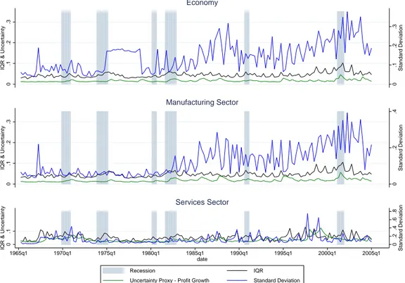
⁹

Figure 2.1 shows IQR, realized and forecast standard deviation per period, estimated as

7

Test results for the presence of ARCH effects using Engle’s Lagrange multiplier (LM) test are reported in the appendix.

8

The change in expected quarterly profit growth in the manufacturing sector is calculated as [(.0182247+1.5*.0003164 *(-20.9759))/(.0182247+.0003164 *(-20.9759))]-1=-0.2863 and analogously in the ser- vices sector.

9

The risk premium is calculated as e.g. 3.026

∗σ

¯

t²

= 1.20% in the services sector.

0.1.2.3 Standard Deviation

0.1.2.3IQR & Uncertainty

Economy

0.2.4 Standard Deviation

0.1.2.3IQR & Uncertainty

Manufacturing Sector

0.2.4.6.8 Standard Deviation

0.1IQR & Uncertainty

1965q1 1970q1 1975q1 1980q1 1985q1 1990q1 1995q1 2000q1 2005q1

date

Recession IQR

Uncertainty Proxy - Profit Growth Standard Deviation

Services Sector

Figure 2.1: IQR, standard deviation and uncertainty proxy for the manufacturing sector, the services sector and the U.S. economy based on normalized profit growth from 1964Q4 to 2005Q1.

Source: Federal Reserve Economic Data (FRED), Compustat Database.

explained above using data on profit growth. Forecast fluctuations are lower than the realized ones in the whole economy, as well as in both sectors. In the manufacturing sector, uncertainty increases after recessions, while this is not as clear for the IQR and standard deviation. In the services sector, the fluctuations do not seem to be associated with the occurrence of recessions. A similar pattern is observable for the IQR and standard deviation.

¹⁰

Figure 2.2 shows somewhat similar results for stock returns. As can be seen in Figures 2.1 and 2.2, IQR and realized standard deviation fluctuate much more than their predicted counterpart which suggests that realizations of profit growth or stock returns further away from the mean occur more frequently than expected.

To compare these uncertainty proxies to more prominent ones, table 2 shows the pairwise correlation coefficients of Macro Uncertainty of Jurado et al. (2015), the V IX used in Bloom (2009), Policy Uncertainty constructed by Baker, Bloom and Davis (2012), this paper’s forecast- based proxies including the Benchmark, the cyclical component of HP-filtered real GDP and a recession indicator. Interestingly, the correlation of the conditional standard deviation forecast

10

Table 2.4 displays the summary statistics of the time-series, and it can be seen that, on average, the expected

conditional standard deviation fluctuates less than the realized standard deviation.

0.05.1.15.2IQR & Uncertainty

Economy

0.05.1.15.2IQR & Uncertainty

Manufacturing Sector

0.1.2.3.4IQR & Uncertainty

1960m1 1970m1 1980m1 1990m1 2000m1 2010m1

date

Recession IQR

Uncertainty Proxy - Stock Returns Standard Deviation

Services Sector

Figure 2.2: IQR, standard deviation and uncertainty proxy for the manufacturing sector, the services sector and the U.S. economy based on stock returns from 1962M8 to 2006M12. Source:

FRED, CRSP.

for profit growth and stock returns are very low or even negative. Moreover, the correlation coefficients of the volatility of stock returns and profit growth are quite different from each other.

Variables P G- M P G- S P G- E SM- M SM- S SM- E Benchmark M acroU nc V IX P olicyU nc GDP Recession

P G- M 1.00

P G- S 0.17 1.00

P G- E 0.87 0.08 1.00

SM- M -0.24 -0.19 -0.05 1.00

SM- S 0.01 0.00 0.09 0.80 1.00

SM- E 0.01 0.00 0.09 0.83 0.98 1.00

Benchmark -0.29 -0.34 -0.18 0.50 0.29 0.32 1.00

M acroU nc -0.04 -0.23 0.03 0.49 0.47 0.47 0.40 1.00

V IX 0.41 0.22 0.36 0.22 0.54 0.53 0.02 0.51 1.00

P olicyU nc 0.28 -0.32 0.35 0.51 0.45 0.44 0.33 0.43 0.41 1.00

GDP -0.30 -0.04 -0.30 -0.20 -0.21 -0.27 -0.30 -0.13 -0.19 -0.34 1.00

Recession 0.13 -0.08 0.14 0.38 0.37 0.41 0.35 0.56 0.41 0.26 -0.41 1.00

Table 2.2: Correlation coefficients of the uncertainty proxies of Jurado et al. (2015), Bloom

(2009), this paper’s forecast proxies, the cyclical component of HP-filtered GDP and a reces-

sion indicator. PG corresponds to the uncertainty proxy based on profit growth, SM to the

uncertainty proxy based on stock market returns; M refers to the manufacturing sector, S to

the services sector and E to the whole economy. Source: Jurado et al. (2015), Bloom (2009),

FRED.

2.4 Conclusion

This paper presents empirical evidence that ex post, profit growth and stock returns fluctuate more than ex ante. Moreover, fluctuations differ across sectors and depend on whether financial or real variables are used to calculate uncertainty. It is important to calibrate theoretical models accordingly, so as not to overstate the role of uncertainty. Uncertainty shocks decrease profit growth and increase stock returns. Variation in the forecast standard deviation of profit growth is not or negatively correlated with the forecast standard deviation in stock returns.

2.5 Appendix

Compustat and CRSP data were downloaded from, http://www.stanford.edu/~nbloom/quarterly2007a .zip.

Federal Reserve Economic Data

• Real GDP - GDPC1

• NBER Recession Indicator - USREC

Jurado et al.’s Uncertainty Proxy

Downloaded from http://www.econ.nyu.edu/user/ludvigsons/jlndata.zip.

Baker, Bloom and Davis’ Uncertainty Proxy

Downloaded from http://www.policyuncertainty.com/us monthly.html.

Tables

lags(p)

Benchmark

PG - M PG - S SR - M SR - S PG - E SR - E

1 0.68 0.01 0.00 0.94 0.38 0.00 0.69

2 0.37 0.03 0.02 0.20 0.08 0.00 0.39

3 0.51 0.03 0.02 0.25 0.16 0.00 0.28

4 0.03 0.02 0.01 0.23 0.14 0.00 0.22

5 0.01 0.02 0.00 0.32 0.00 0.00 0.18

6 0.04 0.02 0.00 0.41 0.00 0.00 0.24

Table 2.3: LM test results (p-values) ARCH effects. H

0

: No ARCH effects. PG refers to profit

growth in the respective sector, SR to stock market returns.

Variable Period Obs. Mean Std. Dev. Min Max Benchmark 1950Q2-2013Q4 255 0.0322011 0.0046514 0.0249326 0.0445141 PG - Uncertainty - M 1965Q1-2005Q1 161 .0165385 .006576 .0098383 .0492981

PG - SD - M 1964Q4-2005Q1 162 0.1218006 0.081629 0.0338525 0.3934643 PG - IQR - M 1964Q4-2005Q1 162 0.0463093 0.0140203 0.027208 0.1056035 PG - Uncertainty- S 1965Q1-2005Q1 161 .0325351 .0123575 .0062582 .0924728

PG - SD - S 1964Q4-2005Q1 162 0.1149527 0.1034904 0.0160815 0.750572 PG - IQR - S 1964Q4-2005Q1 162 0.0534658 0.0229156 0.0144204 0.1328126 PG - Uncertainty - E 1965Q1-2005Q1 161 .016468 .0055934 .0106198 .0460832

PG - SD - E 1964Q4-2005Q1 162 .1422853 .0751701 .0371676 .3778371 PG - IQR -E 1964Q4-2005Q1 162 .044808 .0126902 .0255474 .1030053 SR - Uncertainty - M 1962M9-2006M12 532 .0599957 .0136417 .0376273 .1099285 SR - SD - M 1962M8-2006M12 533 .0794473 .0143971 .0417152 .1368466 SR - IQR - M 1962M8-2006M12 533 .0930246 .0229461 .0293718 .1932621 SR - Uncertainty - S 1962M9-2006M12 532 .0464516 .0083419 .0323597 .0787909 SR - SD - S 1962M8-2006M12 533 .0854849 .0297119 .0232313 .1796676 SR - IQR - S 1962M8-2006M12 533 .1025599 .0479853 .0066667 .3346002 SR - Uncertainty - E 1962M9-2006M12 532 .0421943 .007941 .0297886 .0785901 SR - SD - E 1962M8-2006M15 533 .079327 .0144982 .0553241 .1450797 SR - IQR - E 1962M8-2006M15 533 .0880501 .0219151 .050024 .2045099

Table 2.4: Summary statistics of the Uncertainty Measures. PG corresponds to profit growth in manufacturing (M), services (S), and the whole economy (E), SR to stock market returns.

Uncertainty measure p-val

H0

: Normality Distribution

TFP 0.26 Normal

Profit Growth M 0.00 t(8.93)

Profit Growth S 0.13 Normal

Profit Growth E 0.44 Normal

Stock returns M 0.38 Normal

Stock returns S 0.35 Normal

Stock returns E 0.53 Normal

Table 2.5: Test results - standardized residuals after GARCH-M estimation. Normality tested

using the Kolmogorov-Smirnov test.

Chapter 3

Hump-shape Uncertainty, Agency Costs and Aggregate Fluctuations

3.1 Introduction

This chapter combines uncertainty shocks that rise and fall over time with an agency cost model to provide a further explanation for the observed cyclical fluctuations in output and consumption in the U.S. We model uncertainty (i.e. risk) shocks, changes in the standard deviation around a constant mean, corresponding to the empirical work of Jurado, Ludvigson and Ng (2015) (Macro Uncertainty ) and Ludvigson, Ma and Ng (2016) (Financial Uncertainty): We model the time path of uncertainty shocks to match empirical evidence in terms of shape, duration and magnitude. These previously measured uncertainty shocks using the U.S. data show a hump-shape time path: Uncertainty rises for two years before its decline. Current literature on the effects uncertainty on macroeconomics, including housing, has not accounted for this observation. Consequently, the literature on uncertainty and macroeconomics is divided on the effects and the propagation mechanism of uncertainty on aggregate fluctuations. The models examining the effects of uncertainty in the presence of financial constraints, such as Dorofeenko, Lee and Salyer (2008, henceforth DLS), Chugh (2016), Dmitriev and Hoddenbagh (2015) and Bachmann and Bayer (2013) find uncertainty shock plays quantitatively small role in explaining aggregate fluctuations. Whereas Christiano, Motto and Rostagno (2014), however, find the effect of uncertainty shock on aggregate variables is quantitatively large.

¹

A common theme on all of

1

Some other works that find a large uncertainty effect are Bloom (2009), Bloom, Alfaro and Lin (2016) and

Bloom, Floetotto, Jaimovich, Saporta-Eksten, and Terry (2012), and Leduc and Liu (2015). There are other

works that find a mixed results such as Gilchrist, Sim, and Zakrajsek (2014), who find a small impact on output

and consumption but a large impact on investment.

these aforementioned literature on uncertainty, however, is that a risk shock is characterized by an immediate one time peak after the innovation (i.e. non-hump shape).

This paper shows that when uncertainty rises and falls over time, then the output displays hump-shape with short expansions that are followed by longer and persistent contractions. And because of these longer and persistent contractions in output, uncertainty is, on average, coun- tercyclical. Our model builds on the literature combining uncertainty and financial constraints as in DLS and Bansal and Yaron (2004). Our first calibration exercise builds on DLS as a benchmark, and incorporates a modified Bansal and Yaron (2004) uncertainty structure while the second calibration exercise includes the preferences due to Greenwood, Hercovwitz and Huff- man (1988). Our model’s uncertainty propagation mechanism is, however, different from other models examining the effects of uncertainty in the presence of financial constraints. Unlike other studies that find immediate adverse effects of uncertainty on investment and output following uncertainty shocks that peak immediately after the innovation, we examine the impact of an unexpected shock that does not peak immediately but rises before it falls. In our calibrated models, agents anticipate this hump-shape uncertainty time-path once a shock has occurred.

Thereby, agents respond immediately by increasing investment (i.e. precautionary savings), but

then substantially reduce investment and consumption (and thus output) as more uncertain

times lie ahead. With persistent uncertain periods, both risk premia and bankruptcies increase,

which cause a further deterioration in investment opportunities. A hump shape time-varying

uncertainty accounts for the majority of the variation in the credit channel variables, although

the results are sensitive to the presence and the magnitude of agency costs. In the absence

of agency costs, uncertainty shocks cause expansions because there are no adverse effects for

households. However, in this case, the shocks do not explain any variation in real (<1% in

output and consumption) and financial (<3.5% in the risk premium, the bankruptcy rate and

the relative price of capital) variables. Conversely, the more severe the agency friction, i.e. the

higher the monitoring costs associated with the friction, the more important uncertainty shocks

are. We also show that accounting for hump-shape uncertainty measures can result in a large

quantitative effect of uncertainty shock relative to previous literature. We find hump-shaped

risk shocks account for 5% of the variation in output and 10% and 16% of the variation in

consumption and investment, respectively. Finally, we also analyze the role of the relative risk

aversion parameter and uncertainty. We find the relation between explained variation in output

and consumption and uncertainty is monotonic - a higher coefficient of relative risk aversion

is associated with higher precautionary savings, the associated initial expansion in output is

greater and the subsequent contraction is not as severe.

3.2 Motivation

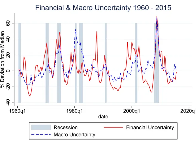
3.2.1 Data

Figure 3.1 shows the Financial Uncertainty and Macro Uncertainty measures proposed by Ju- rado et al. (2015) and Ludvigson et al. (2016) from the period 1960 to 2015. Uncertainty Figure 3.1: Financial Uncertainty and Macro Uncertainty measures from 1960 to 2015, ex- pressed as percent deviation relative to the median.

-40 -20 0 20 40 60 % Deviation from Median

1960q1 1980q1 2000q1 2020q1

date

Recession Financial Uncertainty

Macro Uncertainty

Financial & Macro Uncertainty 1960 - 2015

Source: Jurado et al. (2015) and Ludvigson et al. (2016).

shocks as defined by Jurado et al. (2015) and Ludvigson et al. (2016) (i) raise between 30%

and 73% relative to the median, (ii) exhibit a constant long-run mean and (iii) rise and fall over

time with persistence. For example, during the Great Recession period, the Financial Uncer-

tainty measure peaks after rising for 22 months (2006:12 - 2008:10) and peaks after rising for 11

months (2007:11 - 2008:10) after reaching the median during the great recession period. Other

uncertainty shocks indicated by Ludvigson et al. (2015) peak after rising for 21 months in the

late 1960s (relative to the median, from 1968:7 to the peak in 1970:4); for 26 months in the

mid 1970s (1972:11 - 1975:1); for 23 months in the late 1970s (1978:4 - 1980:3); for 10 months

in the mid 1980s (1986:3 - 1987:1) and for 8 months in the early 1990s (1989:12 - 1990:8).

²

The Macro Uncertainty proxy rose (relative to the median) for 26 months (1972:10 - 1974:12), for 18 months (1978:11 - 1980:5) and for 17 months (2007:5 - 2008:10, with 2007:5, with the trough before the peak slightly above the median). Consequently, the Financial Uncertainty and Macro Uncertainty measures, depicted in Figure 3.1, strongly suggest that uncertainty is not characterized by jumps as in Bloom (2009) but these measured uncertainty shocks show a hump-shape time path.

3.2.2 Empirical Evidence

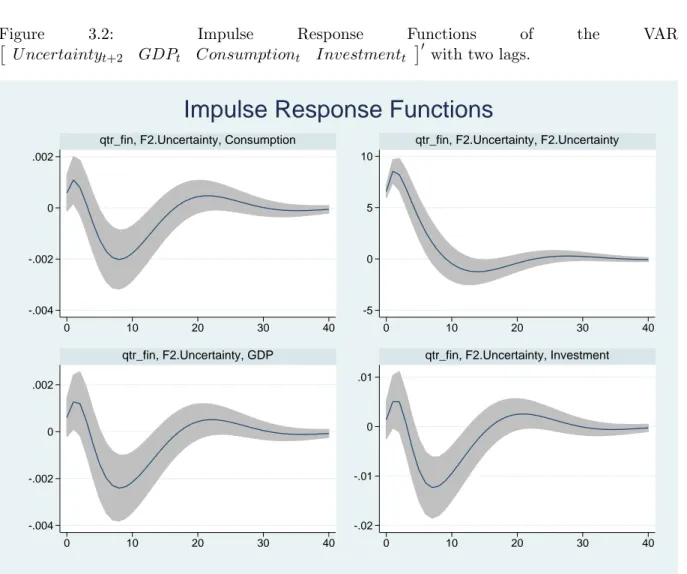
To show corresponding hump-shapes for output, consumption and investment, we take a sim- plistic approach to examining the impact of uncertainty on these real variables, while avoiding a contemporaneous jump in uncertainty. We examine the impact of a shock to future uncer- tainty on today’s output, consumption, investment in a vector autoregression (VAR) model. In doing so, we thus ask, what is the impact on the variables of interest if the anticipated un- certainty is high in the future. We estimate the baseline specification of the VAR using data from 1960Q3 to 2013Q4 with two lags and the cyclical components of output, consumption and investment. Uncertainty is not HP-filtered and expressed as percentage deviation from the me- dian. The results are highly similar if we use the cyclical component of HP-filtered uncertainty or the Macro Uncertainty measure. The vector of variables included in the VAR is given by h

U ncertainty

_t+k

GDP

t

Consumption

t

Investment

t

i

0

with k = 2 in the baseline specifi- cation. Figure 3.2 shows the orthogonalized impulse response functions using this specification.

Financial Uncertainty induces hump-shaped responses in output, consumption and invest- ment. However, as opposed to previous analyses, there are no immediate adverse effects if uncertainty is not restricted to jump unexpectedly from one period to another. Instead, a hump-shaped expansion precedes a pronounced contraction. These results are highly robust to different specifications and different orderings - as long as 2 ≥ k ≥ 8, i.e. if uncertainty is high in the more distant future. If k < 2, the impulse responses show contractions in output, consumption and investment - in line with previous work that analyzes contemporaneous jumps in uncertainty.

³

2

On average, uncertainty peaks for these six shocks after increasing by 48.42%.

3

These results are robust to different lag lengths of the VAR. In a second specification, we also include lagged

delinquency rates on business loans as a proxy for bankruptcies. The impulse response function of delinquencies

is hump-shaped while the responses of output consumption and investment are highly similar for the second

specification.

Figure 3.2: Impulse Response Functions of the VAR U ncertainty

t+2

GDP

t

Consumption

t

Investment

t

0

with two lags.

-.004 -.002 0 .002

-5 0 5 10

-.004 -.002 0 .002

-.02 -.01 0 .01

0 10 20 30 40 0 10 20 30 40

0 10 20 30 40 0 10 20 30 40

qtr_fin, F2.Uncertainty, Consumption qtr_fin, F2.Uncertainty, F2.Uncertainty

qtr_fin, F2.Uncertainty, GDP qtr_fin, F2.Uncertainty, Investment

Impulse Response Functions

Note: Quarterly HP-filtered data from 1960 to 2015. Source: FRED and Ludvigson et al. (2016).

3.3 Model

Carlstrom and Fuerst (1997, henceforth CF) include capital-producing entrepreneurs, who de-

fault if they are not productive enough, into a real business cycles (RBC) model. In the CF

framework, households and final-goods producing firms are identical and perfectly competi-

tive. Households save by investing in a risk-neutral financial intermediary that extends loans

to entrepreneurs. Entrepreneurs are heterogeneous produce capital using an idiosyncratic and

stochastic technology with constant volatility. Unlike CF, DLS introduce stochastic shocks to

the volatility (uncertainty shocks) of entrepreneurs’ technology, such that uncertainty jumps to

its peak and converges back to its steady state. While this approach remedies the procyclical

bankruptcy rates following TFP shocks it introduces countercyclical bankruptcy rates, DLS is

at odds with the measures from Jurado et al. (2015) and Ludvigson et al. (2016). In this

paper, we alter the time path and the magnitude of the shocks introduced in DLS, such that

they correspond more closely to the Macro Uncertainty and Financial Uncertainty measures.

Following these changes, the model displays procyclical consumption, precautionary savings and an increase in output following an initial drop. Our model therefore explains the puzzling ab- sence of precautionary savings following uncertainty shocks in the literature, as raised by Bloom (2014).

In the CF framework, the conversion of investment to capital is not one-to-one because heterogeneous entrepreneurs produce capital using idiosyncratic and stochastic technology. If a capital-producing firm realizes a low technology shock, it declares bankruptcy and the financial intermediary takes over production after paying monitoring costs. The timing of events in the model is as follows:

1. The exogenous state vector of technology and uncertainty shocks, denoted (A

_t

, σ

_ω,t

), is realized.

2. Firms hire inputs of labor and capital from households and entrepreneurs and produce the final good output via a Cobb-Douglas production function.

3. Households make their labor, consumption, and investment decisions. For each unit of investment, the household transfers q

t

units of the consumption goods to the banking sector.

4. With the savings resources from households, the banking sector provide loans to en- trepreneurs via the optimal financial contract (described below). The contract is defined by the size of the loan, i

t

, and a cutoff level of productivity for the entrepreneurs’ technology shock, ¯ ω

_t

.

5. Entrepreneurs use their net worth and loans from the banking sector to purchase the factors for capital production. The quantity of investment is determined and paid for before the idiosyncratic technology shock is known.

6. The idiosyncratic technology shock of each entrepreneur ω

_j,t

is realized. If ω

_j,t

≥ ω ¯

_t

the entrepreneur is solvent and the loan from the bank is repaid; otherwise the entrepreneur declares bankruptcy and production is monitored by the bank at a cost proportional to the input, µi

t

.

7. Solvent entrepreneur’s sell their remaining capital output to the bank sector and use this

income to purchase consumption c

^e_t

and (entrepreneurial) capital z

t

. The latter will in

part determine their net worth n

_t

in the following period.

3.3.1 The Impact of Uncertainty Shocks: Partial Equilibrium

The optimal contract is given by the combination of i

t

and ¯ ω

t

that maximizes entrepreneurs’

return subject to participating intermediaries. Financial intermediaries make zero profits due to free entry

max

it,¯ωt

q

_t

i

_t

f (¯ ω

_t

; σ

_ω,t

) (3.1)

subject to

q

t

i

t

g(¯ ω

t

; σ

ω,t

) ≥ i

t

− n

t

. (3.2) Net worth is defined as

n

_t

= w

^e_t

+ z

_t

(r

_t

+ q

_t

(1 − δ(u

_t

))), (3.3) Entrepreneurs’ share of the expected net capital output is

f (¯ ω

_t

; σ

_ω,t

) = Z

∞

¯ ωt

ω φ(¯ ˜ ω

_t

; σ

_ω,t

)dω − [1 − Φ(¯ ˜ ω

_t

; σ

_ω,t

)]¯ ω

_t

(3.4)

and the lenders’ share of expected net capital output

g(¯ ω

t

; σ

ω,t

) = Z

ω¯t

0

ω φ(¯ ˜ ω

t

; σ

ω,t

)dω + [1 − Φ(¯ ˜ ω

t

; σ

ω,t

)]¯ ω

t

− Φ(¯ ˜ ω

t

; σ

ω,t

)µ. (3.5)

To understand the impact of an uncertainty shock, consider the uncertainty shock in partial equilibrium. For this analysis, q and n are assumed to be fixed while i and ω are chosen. In this setting, uncertainty shocks adversely affect the supply of investment as follows. As σ

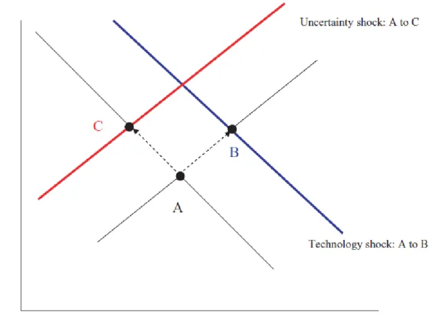
ω

increases, the default threshold ω and lenders’ expected return fall. From the incentive compatibility constraint of entrepreneurs’ problem (3.1), it can be seen that investment has to fall. The effect of an uncertainty shock is summarized graphically, and contrasted with an aggregate technology shock, in Figure 3.3 (taken from DLS).

Whether these results carry over in general equilibrium depends on how the shock is modeled.

They are not overturned following a jump in uncertainty, as analyzed in DLS, or if uncertainty

reaches its peak quickly. In this case, bankruptcies, the associated agency costs, the risk premium

and the price of capital increase. The return to investing falls, saving/investing is less attractive,

so investment and output drop while households substitute into consumption. These results are

overturned, however, following a shock that is hump-shaped if the peak is sufficiently far in the

future.

Figure 3.3: The partial equilibrium impact of an uncertainty shock.

Note: Uncertainty adversely affects capital supply, in contrast to TFP shocks that affect capital demand. Source: DLS.

3.3.2 Modeling Hump-Shaped Uncertainty Shocks

We allow for humps in uncertainty by modifying a subset of equations due to Bansal and Yaron (2004), such that a latent x

_t

variable affects σ

_ω,t

:

log(σ

ω,t+1

) = (1 − ρ

σω

) log(¯ σ

ω

) + ρ

σω

log(σ

ω,t

) + e ε

t+1

(3.6)

e ε

_t+1

= ϕ

_σ

ε

_σ,t+1

+ x

_t+1

(3.7)

x

_t+1

= ρ

_x

x

_t

+ ϕ

_x

ε

_x,t+1

(3.8)

ε

_x,t

, ε

_σ,t ^i.i.d.

∼ N (0, 1), ρ

_σ

, ρ

_x

∈ [0, 1). (3.9)

ε e

t+1

is a composite term that enables uncertainty to jump (innovations in the first term

ϕ

_σ,t+1

ε

_σ,t+1

), as in DLS, or increase over time corresponding to the empirical proxies (innovations

via the latent variable x

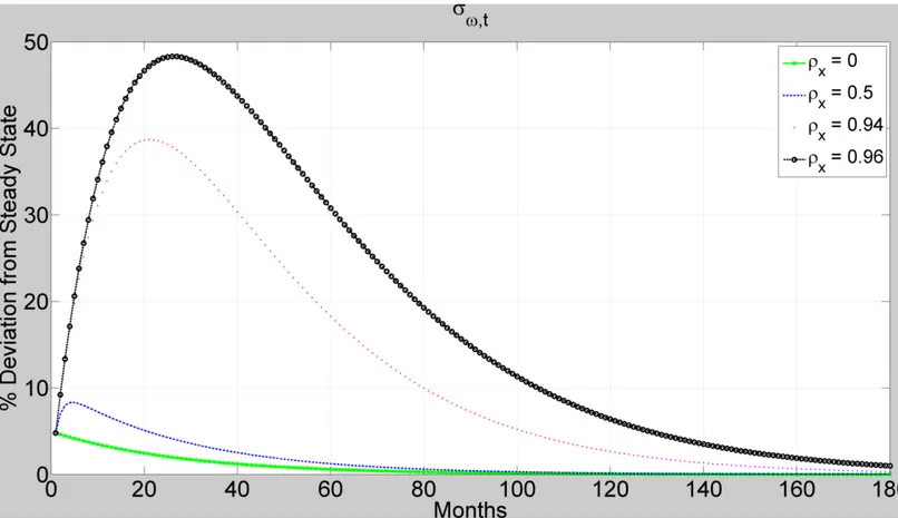
t+1

). Figure 3.4 plots the time series of σ

ω,t

using different persistence

parameters ρ

x

= [0, 0.5, 0.94, 0.96]. The horizontal axis measures time in monthly periods, while the vertical axis shows the percentage deviation from the steady state. Setting ρ

_x

= 0 induces a jump in uncertainty, as analyzed in DLS. The larger ρ

x

, the more pronounced the hump in σ

ω,t

and the longer uncertainty rises before it peaks.

Figure 3.4: Modeling Uncertainty Shocks using different persistence parameters.

Note: The horizontal axis shows monthly periods, while the vertical axis shows the percentage deviation from the steady state. The case with ρ

_x

= 0 corresponds to a jump in uncertainty as analyzed in DLS. The higher ρ

x

, the more pronounced the hump in uncertainty. In the benchmark case with ρ

x

= .96, σ

ω

peaks after rising 25 months, corresponding to the empirical evidence. ρ

_σω

is set to 0.9

^1/3

.

In the benchmark case with ρ

_x

= .96, uncertainty peaks after rising for 25 months, corre- sponding to the empirical evidence. We match the innovation relative to the steady state using the average increase of an uncertainty shock relative to the long-run mean: We set ϕ

_x

= 0.048 such that σ

ω,t

increases by 48% relative to the steady state. Our 48% relative increase com- pares with previous papers as follows. In Bloom (2009) and Bloom, Alfaro and Lin (2016), who use two-state Markov chains to examine the impact of uncertainty, σ

ω

increases by 100%;

in Bloom, Floetotto, Jaimovich, Saporta-Eksten and Terry (2012), σ

_ω

increases between 91%

and 330%. Leduc and Liu (2015) introduce an increase of 39.2% relative to the steady state.

Christiano, Motto and Rostagno (2014), use a combination of un- and anticipated innovations

over a sequence of eight quarters, and their magnitude of these innovations is between 2.83%

and 10% per period. DLS use a 1% innovation, Chugh (2016) and Bachmann and Bayer (2013) examine increases of about 4%, while Dmitriev and Hoddenbagh (2015) use a 3% innovation.

These differences are partially driven by differences in measurement; see also Strobel (2015).

Not surprisingly, greater innovations in uncertainty are associated with a greater role of uncer- tainty in terms of variation explained. One special case is the model of Christiano et al. (2014) who introduce a news component to their shocks: Sims (2015) points out potential issues in using news and variance decompositions. Lee, Salyer and Strobel (2016) show that the news component plays a prominent role regarding the importance of uncertainty.

3.3.3 The Impact of Uncertainty Shocks: General Equilibrium

In order to unambiguously identify the change in the impact of a risk shock that is due to its hump-shape, we insert the shock described in the previous section in a framework identical to DLS. For this reason, the model’s exposition is confined to the agents’ optimization problems.

The representative household’s objective is to maximize expected utility by choosing consump- tion c

t

, labor h

t

and savings k

t+1

, i.e.

{ct,k

max

t+1,ht}^∞₀

E

0

∞

X

t=0

β

^t

ln(c

t

) + ν(1 − h

t

)

(3.10)

subject to

w

t

h

t

+ r

t

k

t

≥ c

t

+ q

t

i

t

(3.11)

k

t+1

= (1 − δ)k

t

+ i

t

(3.12)

with w

t

the wage and r

t

the rental rate of capital. These are equal to their marginal products, as the representative final-good’s producing firm faces a standard, static profit maximization problem

⁴

Kt

max

,Ht,H_t^e

A

_t

K

_t^αK

H

_t^αH

(H

_t^e

)

^{1−αK−αH}

− r

_t

K

_t

− w

_t

H

_t

− w

^e_t

H

_t^e

, (3.13) with K

_t

= k

_t

/η and H

_t

= (1 − η)h

_t

, where η represents the fraction of entrepreneurs in the economy. Total Factor Productivity (TFP) A

t

follows an autoregressive process of order one in logs,

log(A

t+1

) = ρ

A

log(A

t

) + ϕ

A

ε

A,t+1

(3.14)

4

When solving the model, we follow DLS and assume the share of entrepreneurs labor (1

−αK −αH

) is

approximately zero.

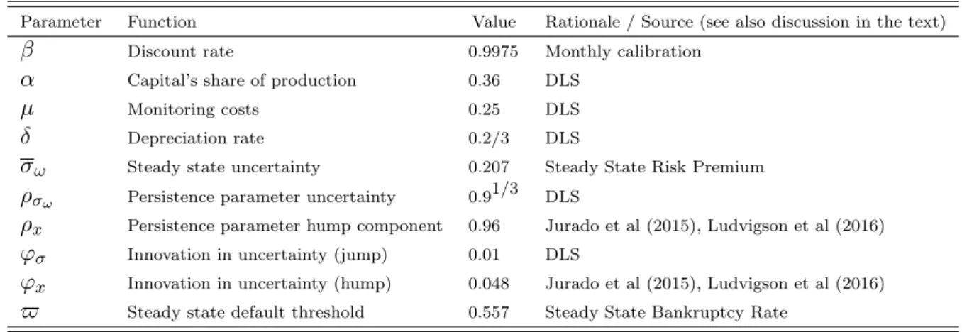
Table 3.1: Benchmark calibration for the monthly frequency.

Parameter Function Value Rationale / Source (see also discussion in the text)

β

Discount rate 0.9975 Monthly calibration

α

Capital’s share of production 0.36 DLS

µ

Monitoring costs 0.25 DLS

δ

Depreciation rate 0.2/3 DLS

σ

_ω Steady state uncertainty 0.207 Steady State Risk Premium

ρ

_σω Persistence parameter uncertainty 0.91/3 DLS

ρ

_x Persistence parameter hump component 0.96 Jurado et al (2015), Ludvigson et al (2016)

ϕ

σ Innovation in uncertainty (jump) 0.01 DLS

ϕ

_x Innovation in uncertainty (hump) 0.048 Jurado et al (2015), Ludvigson et al (2016)

$

Steady state default threshold 0.557 Steady State Bankruptcy Rate

with ε

A,ti.i.d.

∼ N (0, 1). The problem of entrepreneurs is given by

{c^e_t

max

,zt+1}^∞₀

E

₀

∞

X

t=0

(γβ)

^t

c

^e_t

(3.15)

subject to

n

t

= w

^e_t

+ z

t

(r

t

+ q

t

(1 − δ)) (3.16) z

t+1

= n

t

[ f (¯ ω

t

, σ

ω,t

)

1 − q

t

g(¯ ω

t

, σ

ω,t

) ] − c

^e_t

q

t

. (3.17)

The entrepeurs are risk neutral and supply one unit of labor inelastically. Their net worth is defined by sum of labor income w

_t^e

, the income from capital z

_t

r

_t

plus the remaining capital z

t

q

t

(1−δ). At the end of a period, entrepreneurial consumption is financed out of the returns from the investment project, which implies the law of motion (3.17). As the equilibrium conditions are described in DLS, we will not list them in this section.

3.3.4 Calibration

We calibrate the model for the monthly frequency. Otherwise, the frequency of uncertainty would

be too low relative to the empirical counterparts. Table 3.1 shows the benchmark calibration

of the key parameters. The household’s monthly discount rate of 0.9975 implies an annual risk

free rate of about 3%. Following DLS, we set σ

ω

= 0.207, which implies an annual risk premium

of 1.98%. The slight increase in the risk premium, which is 1.87% in DLS, is due to changes

associated with the monthly calibration. The default threshold $ targets an annual bankruptcy

rate of 3.90%, as in DLS.

3.3.5 Cyclical Behaviour

Because of the assumption on entrepreneurs’ productivity, first order approximation of the equilibrium conditions does not impose certainty equivalence. Instead, uncertainty (time-varying second moment) appears in the policy function as a state variable. Figures 3.5 and 3.6 show the impulse response functions following jumps and humps in uncertainty, i.e. the impulse response function for different values of ρ

_x

= [0, 0.5, 0.94, 0.96].

Figure 3.5: Impulse responses of output, household consumption and investment following an uncertainty shock for different persistence parameters, ρ

x

= [0, 0.5, 0.96, 0.979].

Note: The horizontal axis shows monthly periods, the vertical axis shows the percentage devia- tion from the steady state.

If ρ

x

= 0, uncertainty jumps to its peak and an immediate drop in investment and output

ensues, which is expected from the partial equilibrium analysis. Household consumption coun-

terfactually increases as households substitute into consumption. The larger ρ

x

, the longer the

shock takes to peak. Interestingly, there is a threshold value of ρ

_x

that is necessary to induce

prevautionary savings. For instance, ρ

_x

= 0.5 is insufficient to overcome the partial equilib-

rium results and to induce precautionary savings. However, values of ρ

x

corresponding to the

Figure 3.6: Impulse responses of the risk premium, the bankruptcy rate, return to investment and the relative price of capital following an uncertainty shock for different persistence parameters, ρ

_x

= [0, 0.5, 0.96, 0.979].

Note: The horizontal axis shows monthly periods, the vertical axis shows the percentage devia- tion from the steady state, unless indicated otherwise.

uncertainty proxies overturn the partial equilibrium results: An uncertainty shocks is followed by an increase in investment and a hump-shape response of output following the initial drop.

Moreover, in line with the data, consumption is procyclical. The intuition is that immediately after the shock, agency costs are still moderate relative to future periods so investment demand increases, which raises output following the initial drop. While households also substitute into consumption, entrepreneurs greatly reduce consumption after an uncertainty shock because of the increase probability of default and because the higher price of capital results in an increase in investment. The intuition of the model can also be seen in the context of the agency friction.

Figure 3.7 shows the impulse responses for different values of µ.

Without agency friction, µ = 0 (actually, for computational reasons, µ = 0.0001), the

relative price of capital q

_t

is unity. An uncertainty shock, then, induces an expansion in output,

consumption and investment because there are no adverse effects for households. Although

the bankruptcy rate increases, there are no adverse effects. Instead, households benefit from a

more productive investment opportunity. If there are agency costs (µ > 0), the relative price of

capital q

_t

increases, as well as risk premia and bankruptcy rates. In this case, households incur

Figure 3.7: Impulse responses of output, consumption and investment following an uncertainty shock for different magnitudes of monitoring costs, µ=[0.0001, 0.125, 0.2, 0.25].

Note: The horizontal axis shows monthly periods, the vertical axis shows the percentage devia- tion from the steady state.

adverse effects of bankruptcies because of the monitoring costs ˜ Φ(µ

ω

, σ

ω

)µ. Unlike shocks that jump, however, hump-shaped shocks increase investment by around 1.7% relative to the steady state, despite the price-increase associated with the agency friction - overturning the partial equilibrium effects. Since expectations are rational, households know that uncertain times of relatively poor investment opportunities are ahead, so they substantially increase saving as soon as they learn about the shock. As shown in Figure 3.7, the magnitude of the initial increase is inversely related to the size of µ - the higher the monitoring costs, the more capital is destroyed.

Without agency friction, consumption does not increase by much in order to invest more. With agency friction and adverse effects of uncertainty for the households, consumption increases the more the greater µ. The initial increase in investment leads to an expansion in output. However, the subsequent deterioration of conditions in the credit channel leads to a drop in investment and to a contraction in output.

Table 3.2 presents the model’s correlation coefficients. The model produces procyclical con-

sumption and investment if uncertainty is not restricted to jump; the degree of procyclicality

Table 3.2: Correlation coefficients of consumption, investment, bankruptcy rate and uncertainty with output.

Correlation with y Uncertainty Shock c i BR σ

ω

J ump -0.72 0.95 -0.99 -0.69 Hump 0.19 0.88 -0.97 -0.95

Note: BR refers to the bankruptcy rate. The autocorrelation coefficient of uncertainty is ρ

_σω

= 0.9

^1/3

, as in DLS, while uncertainty peaks after rising for 25 months, i.e. ρ

x

= 0.96.

of consumption depends on the persistence of the latent variable, i.e. on how long the shock takes to peak. The bankruptcy rate and uncertainty are strongly countercyclical for both types of risk shocks.

3.4 GHH Preferences and Variable Capital Utilization

The previous section uses the framework of DLS to emphasize the impact of hump-shaped uncer- tainty shocks: precautionary savings, a hump-shape response of output with a short expansion that is followed by a longer and persistent contraction as well as mildly procyclical consump- tion. However, the initial drop in output that precedes the short expansion is much stronger compared to the VAR evidence, while the procyclicality of consumption is senstive to the persis- tence parameter of the latent variable. To remedy these features, we modify the model by using the preferences due to Greenwood, Hercowitz and Huffman (1988), to eliminate effects of labor supply due to changes in consumption, and allow for variable capital utilization. The represen- tative household thus chooses the capital utilization rate u

t

, which is impacts the depretation rate δ(u

_t

), with δ

⁰

(u

_t

), δ

⁰⁰

(u

_t

) > 0. The problem is given by

max

{ct,kt+1,ut,ht}^∞₀

E

₀

∞

X

t=0

β

^t

(1 − ι)

⁻¹

c

_t

− χ h

^1+θ_t

(1 + θ)

1−ι

(3.18)

subject to

w

_t

h

_t

+ r

_t

(u

_t

k

_t

) ≥ c

_t

+ q

_t

i

_t

(3.19)

k

_t+1

= (1 − δ(u

_t

))k

_t

+ i

_t

(3.20)

δ(u

_t

) = δ

₀

+ δ

₁

(u

_t

− 1) + δ

₂

2 (u

_t

− 1)

²

. (3.21)

Table 3.3: Benchmark calibration for the monthly frequency with GHH preferences and variable capital utilization.

Parameter Function Value Rationale / Source (see also discussion in the text)

ι

Coefficient of relative risk aversion 1 Greenwood et al. (1988)

1/θ

Intertemporal elasticity of substitution in labor supply 0.8 Greenwood et al. (1988)

χ

Relative importance of leisure 9.8930 Household works 1/3 of his time

δ

₀ Steady state rate of capital depreciation 0.02/3 DLS

δ

₁ Normalize steady state capital utilization 0.0108 Capital utilization is unity in steady state

δ

2 Sensitivity of capital utilization 0.2 Schmitt-Grohe and Uribe (2008)*

∗

Schmitt-Grohe and Uribe (2008) estimate

δ2

= 0.11 but with a relatively large standard error of 0.26. We set

δ2

slightly higher to restrict capital utilization a bit more given the monthly calibration.

The coefficient of relative risk aversion is given by ι, while 1/θ corresponds to the intertemporal elasticity of substitution in labor supply. χ is the relative importance of leisure. The problem of the final-goods’ producing firms is given by

utK

max

t,Ht,H_t^e

A

_t

(u

_t

K

_t

)

^αK

H

_t^αH

(H

_t^e

)

^{1−αK−αH}

− r

_t

(u

_t

K

_t

) − w

_t

H

_t

− w

_t^e

H

_t^e

. (3.22)

The problem of the entrepreneurs and the optimal contract remain unchanged for the most part, except for the depreciation rate, δ(u

t

). The calibration of the additional parameters is standard and displayed in Table 3.3. The set of equations determining the equilibrium properties are displayed in the Appendix.

3.4.1 Cyclical Behaviour

While the previous section examined an identical economy as DLS, we now consider the impact of the different types of uncertainty shock using the preferences due to Greenwood et al. (1988) to remedy the shortcomings discussed above. We examine the impact on output, investment and household consumption following an innovation that is comparable in magnitude (a 48%

innovation). Consider first the impact of the hump-shaped shock displayed in Figure 3.8. The results are quite robust, although the initial adverse impact on output is much smaller while the brief ensuing expansion is (relative to the DLS framework) more pronounced and persistent.

However, as shown in Table 3.4 below, the procyclicality of consumption is not senstive anymore to uncertainty’s time to peak. In contrast, the results change following a jump in uncertainty.

Most notably, while output drops as expected, investment increases in the first period, mitigating the drop in output, but then drops persistently below its steady state and output falls again.

This is not due to precautionary savings, however. If there is a jump in uncertainty, the amount of

capital destroyed immediately after the shock is much larger compared to a hump-shaped shock

(total costs of default following a jump are more than twice as large after the first two years, which also shows in the bankruptcy rate in Figure 3.9).

⁵

Labor, however, is not substituted for capital (labor perfectly comoves with output given the GHH preferences) but the capital stock is simply replaced. This is also reflected by the marginal product of capital, which increases following a jump in uncertainty whereas it falls following a hump in uncertainty.

Figure 3.8: Impulse responses of output, household consumption and investment following a shock (jump and hump) to uncertainty.

Note: Uncertainty increases by 48% for both types of uncertainty shock. The horizontal axis shows monthly periods, the vertical axis shows the percentage deviation from the steady state.

Table 3.4 presents a further analysis of the equilibrium characteristics. The model produces procyclical consumption and investment for TFP and risk shocks. As discussed above, this is partially due to the GHH preferences, which are also the reason for perfect comovement of labor and output. As opposed to Carlstrom and Fuerst (1997), the bankruptcy rate is counter- cyclical for both types of uncertainty shocks. This similarity conceals the fact that following a hump-shaped uncertainty shock, the bankruptcy rate is initially procyclical and becomes coun- tercyclical only later on. The reason is that uncertainty starts to rise while output still expands due to the initial increase in investment. While uncertainty rises, investment and output de-

5

Not surprisingly, the marginal product of capital increases following a jump while it initially drops (and is

positive only in later periods) following a hump.