Lecture 12: Nonlinear Control
1 Elements of Nonlinear Control
1.1 Equilibrium Point and Linearization
A nonlinear system can be written as
˙
x(t) = f(x(t), u(t))
y(t) = g(x(t), u(t)), (1.1)
wheref(·) andg(·) are nonlinear functions. Recall that (xe, ue) represents anequilibrium point if and only if
0 = f(xe, ue, t)
ye=g(xe, ue, t). (1.2)
As the analysis of the nonlinear system is often difficult, we previously considered such a system in a neighbourhood of its equilibrium points. Mathematically, this translates into considering the Taylor expansion of the functions f(·) and g(·) around the equilibrium points of the system and neglecting high order terms. Let δx =x−xe and δu =u−ue. It holds then
δx˙ =f(xe+δx, ue+δu, t)
= ∂f
∂x xe,ue
δx+∂f
∂u xe,ue
δu+ high order terms
=Aδx+Bδu+ high order terms.
(1.3)
By proceeding analogously for g(·) and neglecting high order terms, one gets δx˙ =Aδx+Bδu
δy =Cδx+Dδu, (1.4)
where C = ∂x∂g xe,ue
and D= ∂u∂g xe,ue
. Remark.
• Note that in general, matrices A, B, C, D are time-varying. However, if f(·), g(·) do not depend explicitly on time t, the linearized model will be time-invariant.
• δx, δu, δy describe a deviation from the equilibrium point. The linearized dynamics are given by
x=xe+δx y=ye+δy u=ue+δu.
(1.5)
1.2 Nominal Stability
During the course Control Systems I, you learned about different stability concepts. More- over, you have learned the differences between internal and external stability: let’s recall them here. Consider a generic nonlinear system defined by the dynamics
˙
x(t) = f(x(t)), t ∈R, x(t)∈Rn, f :Rn×R→Rn. (1.6) 1.2.1 Internal/Lyapunov Stability
Internal stability, also called Lyapunov stability, characterises the stability of the trajec- tories of a dynamic system subject to a perturbation near the to equilibrium. Let now ˆ
x∈Rn be an equilibrium of system (1.6).
Definition 1. An equilibrium ˆx∈Rn is said to be Lyapunov stable if
∀ε >0, ∃δ >0 s.t. kx(0)−xkˆ < δ ⇒ kx(t)−xkˆ < ε. (1.7) In words, an equilibrium point is said to be Lyapunov stable if for any bounded initial condition and zero input, the state remains bounded.
Definition 2. An equilibrium ˆx∈ Rn is said to be asymptotically stable in Ω ⊆Rn if it is Lyapunov stable and attractive, i.e. if
t→∞lim(x(t)−x) = 0,ˆ ∀x(0) ∈Ω. (1.8) In words, an equilibrium is said to be asymptotically stable if, for any bounded initial condition and zero input, the state converges to the equilibrium.
Definition 3. An equilibrium ˆx∈Rn is said to be unstable if it is not stable.
Remark. Note that stability is a property of the equilibrium and not of the system in general.
1.2.2 External/BIBO Stability
External stability, also called BIBO stability (Bounded Input-Bounded Output), charac- terises the stability of a dynamic system which for bounded inputs gives back bounded outputs.
Definition 4. A signal s(t) is said to be bounded, if there exists a finite value B > 0 such that the signal magnitude never exceeds B, that is
|s(t)| ≤B ∀t ∈R. (1.9) Definition 5. A system is said to beBIBO-stable if
ku(t)k ≤ε ∀t ≥0, and x(0) = 0⇒ ky(t)k< δ ∀t≥0, ε, δ ∈R. (1.10) In words, for any bounded input, the output remains bounded.
1.2.3 Stability for LTI Systems
Above, we focused on general nonlinear system. However, in Control Systems I you learned that the output y(t) for a LTI system of the form
˙
x(t) = Ax(t) +Bu(t)
y(t) = Cx(t) +Du(t), (1.11)
can be written as
y(t) = CeAtx(0) +C Z t
0
eA(t−τ)Bu(τ)d(τ) +Du(t). (1.12) The transfer function relating input to output is a rational function
P(s) = C(sI−A)−1B +D= bn−1sn−1+bn−2sn−2+. . .+b0
sn+an−1sn−1+. . .+a0 +d. (1.13) Furthermore, it holds:
• The zeros of the numerator of Equation (1.13) are the zeros of the system, i.e. the values si which fulfill
P(si) = 0. (1.14)
• The zeros of the denominator of Equation (1.13) are the poles of the system, i.e.
the values si which fulfill det(siI−A) = 0, or, in other words, the eigenvalues of A.
One can show, that the following Theorem holds:
Theorem 1. The equilibrium ˆx= 0 of a linear time invariant system is stable if and only if the following two conditions are met:
1. For all λ∈σ(A), Re(λ)≤0.
2. The algebraic and geometric multiplicity of all λ ∈ σ(A) such that Re(λ) = 0 are equal.
Remark. For linear systems, the stability of an equilibrium point does not depend on the point itself. For nonlinear systems, it does.
1.3 Local Stability
Let x=xe be an equilibrium for the autonomous nonlinear system
˙
x(t) = f(x(t)), (1.15)
where f : D → Rn is a continuously differentiable function and D is a neighborhood of xe. Let
A= ∂f
∂x(x) x=xe
. (1.16)
Then:
1. xe is aymptotically stable if Re(λi)<0 for all eigenvalues of A.
2. xe is unstable if Re(λi)>0 for one or more of the eigenvalues of A.
It holds:
• In linear systems, local stability ⇔ global stability.
• In nonlinear systems, this is not true.
1.3.1 Region of Attraction
Definition 6. A function f : Ω ⊆Rn →Rm is said to be Lipschitz on Ω if for K ≥0 it holds
kf(x)−f(y)k
kx−yk ≤K, ∀x, y ∈Ω. (1.17) Definition 7. Letxe be an asymptotically stable equilibrium point of the system ˙x(t) = f(x(t)), wheref(·) is a locally Lipschitz function defined over a domainD ⊂Rn andxe is contained in D. Theregion of attraction(also known as region of asymptotic stability, domain of attraction) is the set of all points x0 ∈ D such that the solution of
˙
x(t) = f(x(t)), x(0) = x0 (1.18)
is defined for all t≥0 and converges toxe ast → ∞. Note that xeis said to be globally asymptotically stable if the region of attraction is the whole spaceRn.
1.4 Lyapunov Stability
1.4.1 Lyapunov Principle - General Systems
1. The Lyapunov Principle is valid for all finite-order systems: as long as the linearized system has no eigenvalues on the imaginary axis.
2. The local stability properties of an arbitrary-order nonlinear system are fully un- derstood once the eigenvalues of the linearization are known.
3. Particularly, if the linearization of a nonlinear system around an isolated equilib- rium point xe is asymptotically stable (or unstable), then this equilibrium is an asymptotically stable (or unstable) equilibrium of the nonlinear system as well. We can but not say that this holds also for the concept of stable system (Re(λ) = 0).
If we are interested in non-local results or in the case of stable systems, we should use the Lyapunov’s direct method.
A scalar function α(p) with α : R+ → R+ is a nondecreasing function if α(0) = 0 and α(p)≥α(q)∀p > q. A function V :Rn+1 →R is a candidate global Lyapunov function if
• The function is strictly positive, i.e., V(x, t)>0 ∀x6= 0,∀t and V(0) = 0 and
• there are two nondecreasing functions α and β which satisfy the inequalities
β(||x||)≤V(x, t)≤α(||x||) (1.19) Remark. If these conditions are not met, only local assumptions can be made.
Theorem 2. The system
˙
x(t) = f(x(t), t), x(t0) =x0 6= 0, (1.20) is globally/locally stable in the sense of Lyapunov if there is a global/local Lyapunov function candidate V(x, t) for which the following inequality holds ∀x(t)6= 0 and∀t:
V˙(x(t), t) = ∂V(x, t)
∂t +∂V(x, t)
∂x f(x(t), t)≤0 (1.21)
Theorem 3. The same system is globally/locally asymptotically stable if there is a global/local Lyapunov function candidate V(x, t) such that −V˙(x(t), t) satisfies all con- ditions of a global/local Lyapunov function candidate.
Remark. In general it is difficult to find suitable functions. A good way to approach the problem is to use physical laws (Lyapunov functions can be seen as generalized energy functions).
For linear systems one can find the Lyapunov function
V(x(t)) =x(t)|·P ·x(t), P =P|>0, (1.22) where P is the solution of the Lyapunov equation
P A+A|P =−Q. (1.23)
For arbitrary Q=Q| >0, a solution to this equation exists if and only if A is a Hurwitz matrix.
Remark. Lyapunov theorems provide sufficient but not necessary conditions!
Example 1. Consider the nonlinear system described by the following differential equa- tions:
˙
x1 =x1x22
˙
x2 =x21x2+ 2x32−6x2. (1.24) a) Linearize the system around the equilibrium x1,e =x2,e = 0 and find matrixA.
b) Can you say something about the stability of the nonlinear system?
c) Evaluate the stability of the nonlinear system using the Lyapunov function V =
1
2(x21+x22) and find the region of attraction about the equilibrium point.
Solution.
1. The linearization matrix A reads A=
∂
∂x1(x1x22) ∂x∂
2(x1x22)
∂
∂x1(x21x2+ 2x32−6x2) ∂x∂
2(x21x2+ 2x32−6x2) (0,0)
=
x22 2x1x2 2x1x2 x21+ 6x22−6
(0,0)
=
0 0 0 −6
.
(1.25)
2. The eigenvalues of matrixAareλ1 = 0 andλ2 =−6. Using the Lyapunov principle, we cannot evaluate the stability of the nonlinear system, since the linearized one is just stable around the equilibrium.
3. The derivative of the Lyapunov function reads V˙ =x1x˙1+x2x˙2
=x1·(x1x22) +x2 ·(x21x2+ 2x32−6x2)
=x21x22+x22x21+ 2x42−6x22
= 2x22·(x21+x22−3).
(1.26)
In order for ˙V to be negative definite, it must hold x21+x22 <3.
1.5 Gain Scheduling
As for most systems stability is guaranteed in some neighborhood of the equilibrium point, we are limited when we design a stabilizing controller. A first method to overcome this problem could be to stabilize the system around each equilibrium point and to design a local controller to get stability. The procedure can be defined as
I) Given the nonlinear system
˙
x(t) = f(x(t), u(t)), (1.27)
choose n equilibrium points (xe,i, ue,i),i= 1, . . . , n.
II) For each of these equilibria, linearize the system and design a local control law ul(x(t)) =ul,e−K(x(t)−xl,e) (1.28) for the linearization.
III) The global control law consists of:
• Choosing the correct control law, as a function of the state: i=σ(x).
• Use that control law: u(x) =uσ(x)(x).
1.6 Feedback Linearization
1.6.1 Input-State Feedback Linearization
Input-state feedback linearization is the ability to use feedback to convert a nonlinear state equation into a linear state equation by canceling nonlinearities. This requires the nonlinear state equation to have the structure
˙
x(t) =Ax(t) +Bβ−1(x(t)) [u(t)−α(x(t))],
y(t) =h(x(t)). (1.29)
where
• The pair (A, B) is controllable.
•
α:Rn→Rp β :Rn →Rp×p
(1.30) are defined on the domain Dx ⊂Rn, which contains the origin.
• The matrix β(x(t)) is assumed to be invertible ∀x∈ Dx.
If the system is in the form presented in Equation 1.29, one can linearize it using the feedback law
u(t) = α(x(t)) +β(x(t))v(t). (1.31) Remark. The form presented in Equation 1.31 has a specific meaning. In fact, it holds
˙
x(t) =Ax(t) +Bβ−1(x(t)) [u(t)−α(x(t))]
=Ax(t) +Bβ−1(x(t)) [α(x(t)) +β(x(t))v(t)−α(x(t))]
=Ax(t) +Bv(t),
(1.32) where v(t) can be chosen with respect to the design constraints. This allows to linearize the dynamics of the system.
1.6.2 Input-State Linearizability
Let z(x(t)) = T(x(t)) be a change of variables (also known as bijection). If both T and T−1 are continuously differentiable, we call it a diffeomorphism. A nonlinear system
˙
x(t) = f(x(t)) + Γ(x(t))u(t), (1.33) where
f :Dx →Rn (1.34)
and
Γ :Dx →Rp×p (1.35)
are sufficiently smooth on a domain Dx ⊂Rn, is said to be input-state linearizable if there exists a diffeomorphism
T :Dx⊂Rn (1.36)
such that
Dz =T(Dx) (1.37)
contains the origin and the change of variables z(x(t)) = T(x(t)) transforms the system into the form
˙
z(x(t)) =Az(x(t)) +Bβ−1(x(t)) [u(t)−α(x(t))], (1.38) with (A, B) controllable and β(x(t)) invertible for all x∈ Dx.
Conditions for Linearizability - General Case But when is this the case? In general, holds
˙
z(x(t)) = ∂T
∂xx(t)˙
= ∂T
∂x [f(x(t)) + Γ(x(t))u(t)].
(1.39)
On the other hand, one can also write
˙
z(t) = Az(t) +Bβ−1(x(t)) [u(t)−α(x(t))]
=AT(x(t)) +Bβ−1(x(t)) [u(t)−α(x(t))]. (1.40) Using Equation 1.39 and Equation 1.40, one can write the general equality which must hold for all x(t) and u(t) in the domain of interest:
∂T
∂x [f(x(t)) + Γ(x(t))u(t)] = AT(x(t)) +Bβ−1(x(t)) [u(t)−α(x(t))]. (1.41) If one sets u(t) = 0, one can split the equation into two:
∂T
∂xf(x(t)) =AT(x(t))−Bβ−1(x(t))α(x(t))
∂T
∂xΓ(x(t)) =Bβ−1(x(t)).
(1.42)
Each correct transformation T(·) must satisfy the partial differential equations given in Equation 1.42.
Having T(x(t)) which fulfills these partial differential equations is a necessary and suf- ficient conditions that a transformation from the form in Equation 1.33 to the form in Equation 1.38 exists.
Conditions for Linearizability - Single Input
With a single input (p = 1), one can define a linear transformation ξ(x(t)) = M z(x(t)) with M invertible and write
ξ˙=M AM−1ξ+M Bβ−1(x(t)) [u(t)−α(x(t))]. (1.43) We choose M such that the controller canonical form can be written as
Ac+Bcγ| Bc Cc Dc
=
0 1 0 . . . 0 0
0 0 1 0 . . . 0 0
... . .. ... ... . .. ...
0 . . . 0 1 0 0
0 . . . 0 1 0
−γ0 −γ1 . . . − −γn−2 −γn−1 1 c0 . . . cm 0 . . . 0 0
. (1.44)
This means
M AM−1 =Ac+Bcγ| (1.45)
and
M B =Bc. (1.46)
The term
Bcγ|ξ=Bcγ|M T(x(t)) (1.47) is included into the nonlinearity
Bcβ−1(x(t))α(x(t)), (1.48)
which allows to reformulate the partial differential equations as
AcT(x(t))−Bcβ−1(x(t))α(x(t)) =
T2(x) T3(x)
... Tn−1(x)
Tn(x)
(1.49)
and
Bcβ−1(x(t)) =
0 0 ... 0
1 β(x(t))
. (1.50)
Finally, one can write
∂T1
∂x(t)f(x(t)) = T2(x(t))
∂T2
∂x(t)f(x(t)) = T3(x(t)) ...
∂Tn−1
∂x(t)f(x(t)) = Tn(x(t))
∂Tn
∂x f(x(t)) = −α(x(t)) β(x(t))
(1.51)
and
∂T1
∂x γ(x(t)) = 0
∂T2
∂x γ(x(t)) = 0 ...
∂Tn−1
∂x γ(x(t)) = 0
∂Tn
∂x γ(x(t)) = 1 β(x(t))
(1.52)
1.7 Examples
Example 2. 1. Consider the continuous-time system
˙
x(t) = 0.5x(t), x(t)∈R, (1.53)
and the test function
V(x) = 2x. (1.54)
Which of the following statements is true?
V(x) is a Lyapunov function for this system and therefore the system is asymp- totically stable.
V(x) is not a Lyapunov function for this system and therefore the system is not stable.
V(x) is not a Lyapunov function for this system. Furthrermore, given this information, we cannot conclude anything about the stability of the system.
2. Which of the following functions are positive definite V(x) =x1(t)2+x2(t)2.
V(x) =x1(t)2.
V(x) = (x1(t) +x2(t))2.
V(x) =−x1(t)2−(3x1(t) + 2x2(t))2. V(x) =x1(t)x2(t) +x2(t)2.
V(x) =x1(t)2+ 1+x2x2(t)2
2(t)2. 3. You are given the nonlinear system
˙
x1(t) = x1(t)x2(t)2
˙
x2(t) = x1(t)2x2(t) + 2x2(t)3−6x2(t). (1.55) Evaluate the stability of the origin using the Lyapunov function
1
2(x21(t) +x2(t)2). (1.56) The largest region of attraction of the system is{x(t)∈R2|x1(t)2+x2(t)2 ≤3}.
The largest region of attraction of the system is√ {x(t) ∈ R2|x1(t)2+x2(t)2 ≤ 3}.
The largest region of attraction of the system is{x(t)∈R2|x1(t)2+x2(t)2 ≤2}.
The largest region of attraction of the system is√ {x(t) ∈ R2|x1(t)2+x2(t)2 ≤ 2}.
None of the above.
Solution.
1.
V(x) is a Lyapunov function for this system and therefore the system is asymp- totically stable.
V(x) is not a Lyapunov function for this system and therefore the system is not stable.
3
V(x) is not a Lyapunov function for this system. Furthermore, given this information, we cannot conclude anything about the stability of the system.Solution: The test function is not a Lyapunov function. One can verify this by observing that:
• V(x) is not a positive definite function or
•
V˙(x) = dV dx
dx(t) dt
= ∂V
∂xx(t)˙
= 2·0.5·x
=x
(1.57)
is not a negative definite function.
Since V(x) is not a Lyapunov function, we cannot conclude anything about the stability of the system. Moreover, we know that the system is unstable only from the positive eigenvalue λ1 = 0.5, and not from V(x).
2.
3
V1(x(t)) =x1(t)2 +x2(t)2. V2(x(t)) =x1(t)2.V3(x(t)) = (x1(t) +x2(t))2.
V4(x(t)) =−x1(t)2 −(3x1(t) + 2x2(t))2. V5(x(t)) =x1(t)x2(t) +x2(t)2.
Solution:
• V1(x(t))>0 ∀x(t)6= 0 andV1(x(t)) = 0 if x= 0.
• V2(x(t)) > 0 ∀x(t) 6= 0 and V2(x(t)) = 0 if x1 = 0. This still holds for any x2(t)6= 0, which makes V2(x(t)) positive semi-definite.
• V3(x(t))≥0∀x(t), but can be 0 as soon as x1(t) =−x2(t).
• V4(x(t))<0 ∀x(t)6= 0.
• As soon as x1(t)x2(t)< x2(t)2, V5(x(t))<0.
3. The largest region of attraction of the system is{x(t)∈R2|x1(t)2+x2(t)2 ≤3}.
The largest region of attraction of the system is√ {x(t) ∈ R2|x1(t)2+x2(t)2 ≤ 3}.
The largest region of attraction of the system is{x(t)∈R2|x1(t)2+x2(t)2 ≤2}.
The largest region of attraction of the system is√ {x(t) ∈ R2|x1(t)2+x2(t)2 ≤ 2}.
3
None of the above.Solution: It holds V˙(x1(t), x2(t)) = ∂V
∂x1
∂x1
∂t + ∂V
∂x2
∂x2
∂t
=x1(t) x1(t)x2(t)2
+x2(t) x1(t)2x2(t) + 2x2(t)3−6x2(t)
= 2x1(t)2x2(t)2+ 2x2(t)4−6x2(t)2
= 2x2(t)2 x1(t)2+x2(t)2−3 .
(1.58)
In order to find the region of attraction for which the system is asymptotically stable, ˙V(x) must be negative definite. This is the case if
{x(t)∈R2|x1(t)2+x2(t)2 <3}. (1.59) This ensures that the region of attraction for the origin is at least the one presented in Equation 1.59. However, the choice of another Lyapunov function could result in a larger region of attraction. This explains why none of the first four answers is correct.
Example 3. You are given the system
˙
x(t) =f(x(t)) +gu(t), (1.60)
with
f(x(t)) =
x2(t)
−asin(x1(t))−b(x1(t)−x3(t)) x4(t)
c(x1(t)−x3(t))
,
0 0 0 d
(1.61)
where a,b,cand d are positive constants. We want to find a diffeomorphismus such that T1(x(t)) fulfills:
∂Ti
∂xg = 0, i= 1,2,3; ∂T4
∂x g 6= 0. (1.62) The system has clearly an equilibrium point at x= 0. From the first condition
∂T1
∂x g = 0, (1.63)
one knows that
∂T1
∂x4g = 0. (1.64)
This means that one must choose T1(x(t)) independent ofx4(t). Using this, one can write T2(x(t)) = ∂T1
∂x1x2(t) + ∂T1
∂x2 (−asin(x1(t))−b(x1(t)−x3(t)) + ∂T1
∂x3x4(t). (1.65) From the second condition
∂T2
∂x g = 0, (1.66)
one knows that
∂T1
∂x4 = 0. (1.67)
This implies
∂T2
∂x4
= 0⇒ ∂T1
∂x3
= 0. (1.68)
T1(x(t)) needs to be independent of x3(t) and hence T2(x(t)) = ∂T1
∂x1
x2(t) + ∂T1
∂x2
(−asin(x1(t))−b(x1(t)−x3(t)), (1.69) and
T3(x(t)) = ∂T2
∂x1x2(t) + ∂T2
∂x2 (−asin(x1(t))−b(x1(t)−x3(t)) + ∂T2
∂x3x4(t). (1.70) From the third condition
∂T3
∂x g = 0, (1.71)
one knows that
∂T3
∂x4 = 0. (1.72)
This implies
∂T3
∂x4 = 0⇒ ∂T2
∂x3 = 0 ⇒ ∂T1
∂x2 = 0. (1.73)
T1(x(t)) needs to be independent of x2(t) and hence T4(x(t)) = ∂T3
∂x1x2(t) + ∂T3
∂x2 (−asin(x1(t))−b(x1(t)−x3(t)) + ∂T3
∂x3x4(t). (1.74) The last condition
∂T4
∂xg 6= 0 (1.75)
is satisfied if
∂T3
∂x3 6= 0⇒ ∂T2
∂x2 6= 0 ⇒ ∂T1
∂x1 6= 0. (1.76) With T1(x(t)) =x1(t), one can write
z1(x(t)) = T1(x(t)) =x1(t) z2(x(t)) = T2(x(t)) =x2(t)
z3(x(t)) = T3(x(t)) =−asin(x1(t))−b(x1(t)−x3(t)) z4(x(t)) = T4(x(t)) =−ax2(t) cos(x1(t))−b(x2(t)−x4(t)).
(1.77)
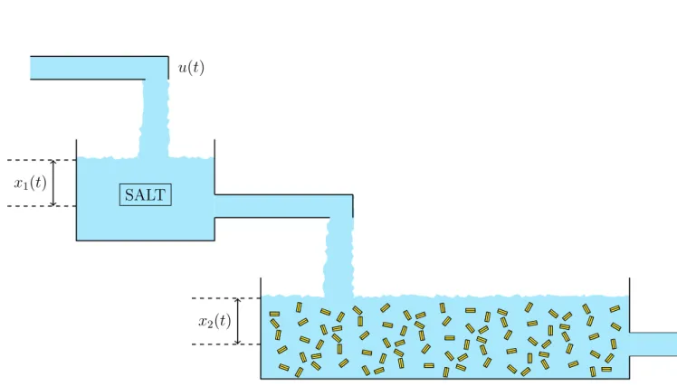
Example 4. Your SpaghETH startup, which cooks pasta on the polyterrasse everyday, is growing every week more and although no particular production issues occur you are concerned about ecology. Since each tank of pasta you cook needs water and a correct salt seasoning for it to taste that delicious, you need a lot of salt and water, which are often wasted. For this reason, you open a research branch in your startup which decides to design a duct-hydraulic system to counteract the waste of water and salt. The idea is to use a two water tank system, which helps you seasoning the water and changing it, without substituting the whole pot. The dynamics of the system are given by
˙
x1(t) = 1 +u(t)−p
1 +x1(t)
˙
x2(t) =p
1 +x1(t)−p
1 +x2(t) y=x2(t).
(1.78) a) Linearize the nonlinear system around the equilibrium
x1,eq(t) x2,eq(t) ueq(t)
= 3 3 1
. (1.79)
b) Determine the coordinate transformation such that the system can be written in the form
˙
z1(t) =z2(t)
˙
z2(t) =α(z) +β(z)u(t) y(t) =z1(t).
(1.80)
c) Find a feedback control law by exactly linearizing the system.
x2(t) x1(t)
SALT u(t)
Figure 1: Sketch of the system.
Solution.
a) It holds
A=
− 1
2√
1+x1(t) 0
1 2√
1+x1(t) − 1
2√
1+x2(t)
x
1,eq(t)=x2,eq(t)=3
= −14 0
1 4 −14
! ,
B = 1
0
, C = 0 1
, D= 0.
(1.81)
b) By choosing the states
z(t) =
z1(t) z2(t)
= y(t)
˙ y(t)
, (1.82)
one gets
˙
z1(t) =z2(t)
˙
z2(t) = ∂
∂ty(t)˙
= ∂
∂tx˙2(t)
= 1
2p
1 +x1(t)x˙1(t)− 1 2p
1 +x2(t)x˙2(t)
= 1
2p
1 +x1(t)
1 +u(t)−p
1 +x1(t)
− 1
2p
1 +x2(t)
p1 +x1(t)−p
1 +x2(t)
= 1 2
1
p1 +x1(t) −
p1 +x1(t) p1 +x2(t)
!
+ u(t)
2p
1 +x1(t).
(1.83) Furthermore, we know
z1(t) =y(t) = x2(t) z2(t) = ˙y(t) = ˙x2(t)
=p
1 +x1(t)−p
1 +x2(t),
(1.84) from which it follows
x2(t) = z1(t) p1 +x1(t) = z2(t) +p
1 +z1(t) (1.85)
Plugging Equation 1.85 into Equation results in
˙
z1(t) = z2(t)
˙
z2(t) = 1 2
1 z2(t) +p
1 +z1(t) −z2(t) +p
1 +z1(t) p1 +z1(t)
! +1
2
u(t) z2(t) +p
1 +z1(t)
=α(z(t)) +β(z(t))u(t).
(1.86)
c) With the form obtained in Equation 1.86, one can write z˙1(t)
˙ z2(t)
= 0 1
0 0
z1(t) z2(t)
+
0 1
v(t), (1.87)
where u(t) = 1
β(z(t))(v(t)−α(z(t)))
= 2(z2(t) +p
1 +z1(t)) v(t)− 1 2
1 z2(t) +p
1 +z1(t) −z2(t) +p
1 +z1(t) p1 +z1(t)
!!
. (1.88)
References
[1] Hassan K. Khalil, Nonlinear Systems. Michigan State University.