Lumpy Investment and State- Dependent Pricing in General Equilibrium

IHS Economics Series Working Paper 239

May 2009

Lumpy Investment and State- Dependent Pricing in General

Equilibrium

Michael Reiter

Tommy Sveen

Lutz Weinke

Impressum Author(s):

Michael Reiter, Tommy Sveen, Lutz Weinke Title:

Lumpy Investment and State-Dependent Pricing in General Equilibrium ISSN: Unspecified

2009 Institut für Höhere Studien - Institute for Advanced Studies (IHS) Josefstädter Straße 39, A-1080 Wien

E-Mail: o ce@ihs.ac.at ffi Web: ww w .ihs.ac. a t

All IHS Working Papers are available online: http://irihs. ihs. ac.at/view/ihs_series/

This paper is available for download without charge at:

https://irihs.ihs.ac.at/id/eprint/1918/

Lumpy Investment and State-Dependent Pricing in General Equilibrium

Michael Reiter, Tommy Sveen, Lutz Weinke

239

Reihe Ökonomie

Economics Series

239 Reihe Ökonomie Economics Series

Lumpy Investment and State-Dependent Pricing in

General Equilibrium

Michael Reiter, Tommy Sveen, Lutz Weinke May 2009

Institut für Höhere Studien (IHS), Wien

Institute for Advanced Studies, Vienna

Contact:

Michael Reiter

Department of Economics and Finance Institute for Advanced Studies Stumpergasse 56

1060 Vienna, Austria

: +43/1/599 91-154 email: michael.reiter@ihs.ac.at Tommy Sveen

Monetary Policy Department Norges Bank

Bankplassen 2 P.O.Box 1179 Sentrum 0107 Oslo, Norway

email: tommy.sveen@norges-bank.no Lutz Weinke

Department of Economics Duke University

Durham, NC 27708, USA email: weinkel@duke.edu

and Department of Economics and Finance Institute for Advanced Studies, Vienna

Founded in 1963 by two prominent Austrians living in exile – the sociologist Paul F. Lazarsfeld and the economist Oskar Morgenstern – with the financial support from the Ford Foundation, the Austrian Federal Ministry of Education and the City of Vienna, the Institute for Advanced Studies (IHS) is the first institution for postgraduate education and research in economics and the social sciences in Austria. The Economics Series presents research done at the Department of Economics and Finance and aims to share ―w ork in progress ‖ in a timely way before formal publication. As usual, authors bear full responsibility for the content of their contributions.

Das Institut für Höhere Studien (IHS) wurde im Jahr 1963 von zwei prominenten Exilösterreichern –

dem Soziologen Paul F. Lazarsfeld und dem Ökonomen Oskar Morgenstern – mit Hilfe der Ford-

Stiftung, des Österreichischen Bundesministeriums für Unterricht und der Stadt Wien gegründet und ist

somit die erste nachuniversitäre Lehr- und Forschungsstätte für die Sozial- und Wirtschafts-

wissenschaften in Österreich. Die Reihe Ökonomie bietet Einblick in die Forschungsarbeit der

Abteilung für Ökonomie und Finanzwirtschaft und verfolgt das Ziel, abteilungsinterne

Diskussionsbeiträge einer breiteren fachinternen Öffentlichkeit zugänglich zu machen. Die inhaltliche

Verantwortung für die veröffentlichten Beiträge liegt bei den Autoren und Autorinnen.

Abstract

The lumpy nature of plant-level investment is generally not taken into account in the context of monetary theory (see, e.g., Christiano et al. 2005 and Woodford 2005). We formulate a generalized (S,s) pricing and investment model which is empirically more plausible along that dimension. Surprisingly, our main result shows that the presence of lumpy investment casts doubt on the ability of sticky prices to imply a quantitatively relevant monetary transmission mechanism.

Keywords

Lumpy investment, sticky prices

JEL Classification

E22, E31, E32

Comments

We have benefited from comments at the ESSIM 2008, European Central Bank, 5. Christmas Meeting

of German-speaking Economists Abroad, 14. International Conference on Computing in Economics

and Finance, Humboldt-Universität zu Berlin, IGIER-Università Bocconi, Institute for Advanced Studies

(Vienna), Norges Bank, Swiss National Bank and Universitat Pompeu Fabra. We also thank Rüdiger

Bachmann, Jordi Galí, Bjørn Sandvik and Fredrik Wulfsberg for useful comments. Part of this work was

done while Sveen was visiting CREI and Universitat Pompeu Fabra. He thanks them for their

hospitality. The usual disclaimer applies. The views expressed in this paper are those of the authors

and should not be attributed to Norges Bank.

Contents

1 Introduction 1

2 The Model 3

2.1 Households ... 3

2.2 Firms ... 5

2.3 Market Clearing and Monetary Policy ... 6

2.4 Baseline Calibration ... 7

2.5 Numerical Method ... 8

3 Results 8 3.1 Steady State ... 8

3.2 The Monetary Transmission Mechanism ... 13

4 Conclusion 20

References 21

Appendix: Numerical Method 24

1 Introduction

Many microeconomic decisions are lumpy in nature. Caballero and Engel (2007) note that examples include not only infrequent price adjustment by …rms but also investment decisions, durable purchases, hiring and …ring decisions, inventory ac- cumulation, and many other economic variables of interest. We develop a dynamic stochastic general equilibrium (DSGE) framework featuring sticky prices combined with monopolistic competition and lumpy investment. In this way we integrate the New Keynesian (NK) framework, which is the workhorse of current monetary policy analysis, with the dominant approach of the recent micro-founded investment liter- ature. The combination of these two literatures allows us to address the following question. Do NK models still deliver a quantitatively relevant monetary transmis- sion mechanism

when they are augmented by a standard micro-founded investment model? Surprisingly, our answer is no. Let us put this result into perspective. Tra- ditionally, capital accumulation has been ignored in NK theory.

Woodford (2003, p. 352) comments on this modeling choice: ‘[...] while this has kept the analysis of the e¤ects of interest rates on aggregate demand quite simple, one may doubt the accuracy of the conclusions obtained, given the obvious importance of variations in investment spending both in business ‡uctuations generally and in the transmission mechanism for monetary policy in particular.’ By now, prominent treatments of the monetary transmission mechanism do feature endogenous capital accumulation (see, e.g., Christiano et al. 2005 and Woodford 2005). We observe, however, that those models simply brush away the lumpy nature of plant level investment. More impor- tantly, our main result shows that this is crucial for the ability of monetary DSGE models to generate a quantitatively relevant monetary transmisson mechanism.

We assume stochastic …xed adjustment costs for both price-setting and invest- ment. This way of modeling state-dependent decisions in the context of general equilibrium analyses has been employed both in monetary economics (see, e.g., Dot- sey et al. 1999) and in the lumpy investment literature (see, e.g., Thomas 2002 and Khan and Thomas 2008). Under the baseline calibration we …nd that the impact responses of investment and output to monetary policy shocks are way too large and that there is essentially no persistence. How does this result change in the presence

1

The monetary transmission mechanism is generally viewed as being the hallmark of monetary economics. See, e.g., Woodford (2003, p. 6) and Galí (2008, p. 1).

2

See, e.g., Clarida et al. (1999).

1

of Calvo (1983) pricing? In that case the impact responses of real variables to a monetary policy shock become even larger and there is essentially no gain in terms of persistence. We also show that there exist speci…cations of the price adjustment cost for which the impact responses of the real variables are reduced with respect to our baseline calibration but in no case do we …nd persistent e¤ects of monetary policy shocks or a realistic split of output between investment and consumption.

Taken together our main result therefore suggests that the presence of an empir- ically plausible investment decision at the …rm level casts doubt on the ability of sticky prices to imply a quantitatively relevant monetary transmission mechanism.

The (S,s) nature of investment decisions is the crucial to understand this result.

In response to an expansionary monetary policy shock …rms choose to undertake some of the investment activity that they would have otherwise done later. This is important for two reasons. First, the impact investment response to the shock becomes very large. Second, the distribution of …rms in the economy is altered in such a way that investment in subsequent periods is reduced. This explains both the enormous size of the impact response of investment to a monetary disturbance (which is driving the large output responses) and the almost complete lack of per- sistence in the dynamic consequences of that shock. Finally, the di¤erence in results between (S,s) pricing and price-setting à la Calvo is a consequence of an extensive margin e¤ect, as analyzed in Caballero and Engle (2007).

The technical di¢ culties implied by simultaneous (S,s) decision making in the context of a general equilibrium model are quite substantial. This explains why most existing theoretical analyses in the related literature have focused on one par- ticular lumpy decision at a time. For instance, Thomas (2002), Gourio and Kashyap (2007), Bachmann et al. (2008) and Khan and Thomas (2008) analyze aggregate consequences of lumpy investment in the context of RBC models, whereas Dotsey et al. (1999), Dotsey and King (2005), Midrigan (2006), Bakhshi et al. (2007), Golosov and Lucas (2007), Dotsey et al. (2008), Gertler and Leahy (2008), and Nakamura and Steinsson (2008) focus exclusively on the role of state-dependent pricing for aggregate dynamics. We overcome those di¢ culties by using the method developed in Reiter (2008, 2009). Another paper which integrates (S,s) pricing and investment decisions in general equilibrium is Johnston (2008).

We regard his work as comple-

3

Kryvtsov and Midrigan (2009) integrate pricing and inventory decisions in the context of a menu cost model. They use their model to analyze the behavior of inventories in the aftermath of monetary policy shocks.

2

mentary to ours. He assumes a stationary process for the growth rate of real balances (combined with an interest rate inelastic demand for real balances), whereas we con- sider an interest rate rule for the conduct of monetary policy. Moreover Johnston (2008) ensures tractability of his framework by making assumptions which limit the extent to which the timing of pricing decisions is chosen optimally.

Our model is therefore not nested with his framework. Johnston (2008) …nds that the presence of lumpy investment lowers somewhat the persistence in the real consequences of monetary disturbances (with respect to a version of his model in which capital is endogenous but not lumpy). Our analysis shows, however, that the consequences of lumpy investment are dramatic in an economic environment that is otherwise closer to standard textbook treatments of the monetary transmission mechanism.

The remainder of the paper is organized as follows. Section 2 outlines the model.

Section 3 presents the results and Section 4 concludes.

2 The Model

2.1 Households

Households are assumed to have access to a complete set of …nancial markets. The representative household has the following period utility function

U (C

; L

) = ln C

+

1 (1 L

)

;

which is separable in its two arguments C

and L

. The former denotes a Dixit- Stiglitz consumption aggregate while the latter is meant to indicate hours worked.

Our notation re‡ects that a household’s time endowment is normalized to one per period and throughout the analysis the subscript t is used to indicate that a variable is dated as of that period. The inverse of the steady state labor supply elasticity is given by

and we adopt the convention that a variable without time subscript indicates its steady state value. Parameter is a scaling parameter whose role will be discussed below. The consumption aggregate reads

C

Z

C

(i)

di

1

; (1)

4

Speci…cally, he assumes that if a …rm wants to adjust its capital, it must also adjust its price. In addition he assumes that capital is installed and becomes productive immediately after purchase.

3

where is the elasticity of substitution between di¤erent varieties of goods C

(i).

The associated price index is de…ned as follows

P

Z

P

(i)

di

1 1

; (2)

where P

(i) is the price of good i. Requiring optimal allocation of any spending on the available goods implies that consumption expenditure can be written as P

C

. Households are assumed to maximize expected discounted utility

E

X

k=0

k

U (C

; L

) ;

where is the subjective discount factor. The maximization is subject to a sequence of budget constraints of the form

P

C

+ E

f Q

D

g D

+ P

W

L

+ T

; (3) where Q

denotes the stochastic discount factor for random nominal payments and D

gives the nominal payo¤ associated with the portfolio held at the end of period t. We have also used the notation W

for the real wage and T

is nominal dividend income resulting from ownership of …rms.

The labor supply equation implied by this structure takes the standard form

C

(1 L

) = W

; (4)

and the consumer Euler equation is given by Q

= C

C

1

; (5)

where Q

Q

is the real stochastic discount factor, and

Pt

is the gross rate of in‡ation between periods t and t+1. We also note that E

f Q

g = R

, where R

is the gross risk free nominal interest rate.

4

2.2 Firms

There is a continuum of …rms and each of them is the monopolistically competitive producer of a di¤erentiated good. Each …rm i 2 [0; 1] is assumed to maximize its market value subject to constraints implied by the demand for its good and the production technology it has access to. Moreover each …rm faces random …xed costs of price and capital adjustment. This implies generalized (S; s) rules for price-setting and for investment. The central question of the present paper regards the monetary transmission mechanism. Monetary policy shocks are therefore assumed to be the only source of aggregate uncertainty. In each period the time line is as follows.

1. The cost of adjusting the price as well as the monetary policy shock realize.

2. The …rm changes its price (or not).

3. Production takes place.

4. The cost of adjusting the capital stock realizes.

5. The …rm invests (or not).

Let us now be more speci…c about the above mentioned constraints. Each …rm i has access to the following Cobb-Douglas production function

Y

(i) = L

(i)

K

(i)

; (6) where

and

denote the shares of labor and capital in production. In order to invest or to change its price a …rm must pay a …xed cost. More precisely, we denote the cost functions for investment and for price-setting by C

(i) and C

(i). They are both measured in units of the aggregate good and are given by

C

(K

(i) ; K

(i) ; c

) =

( K

(i) if K

(i) = (1 ) K

(i) ;

K

(i) (1 ) K

(i) + c

otherwise. (7) C

(P

(i) ; P

(i) ; c

) =

( 0 if P

(i) = P

(i) ;

c

otherwise. (8)

The realizations of the capital and price adjustment costs are denoted c

and c

, respectively, and is the rate of depreciation net of maintenance, . The cost distri- bution functions are assumed to take the general form G ( ) = c

+ c

tan (c

c

) ;

5

which is parametrized by c

, c

, c

and c

. For the price adjustment cost we follow Dotsey et al. (1999) in assuming an inverted S-shaped distribution, whereas we assume a linear distribution function for capital adjustment costs, which is a con- ventional choice in that literature (see, e.g., Thomas 2002 and Khan and Thomas 2008).

Cost-minimization on the part of households and …rms implies that demand for good i is given by

Y

(i) = P

(i)

P

Y

; (9)

where aggregate demand is Y

= C

+ I

+ C

, which consists of consumption, aggregate investment, I

R

0

C

(i) di, and aggregate price-setting costs, C

= R

0

C

(i) di.

Each …rm maximizes its market value E

X

k=0

Q

f

(i) C

(i) C

(i) W

g ; (10)

where

(i)

t

Y

(i) W

L (i) is the gross operating surplus, and denotes a

…xed cost which is measured in units of labor and whose role will be explained when we discuss our calibration. The maximization is done subject to the constraints in equations (6), (7), (8) and (9).

2.3 Market Clearing and Monetary Policy

The goods market clearing condition reads

Y

(i) = Y

(i) for all i. (11) Clearing of the labor market requires

Z

0

[L

(i) + ] di = L

. (12)

5

The parameter values for the adjustment cost distribution functions are calibrated as follows:

Inverted S-shaped distribution: c

= 438:4=B

; c

= 1:26 and for the linear distribution: c

= 150:9=B

and c

= 0:3, where B

= 0:00467 and B

= 0:0115 are the respective upper bounds.

They are chosen to target some empirical regularities on capital adjustment and price-setting at the …rm level. We will come back to this. Finally, parameters c

and c

are chosen in each case to guarantee that G (0) = 0 and G (B

) = 1, whith j 2 f p; k g .

6

To close the model we assume a Taylor-type rule for the conduct of monetary policy

R

= (R

)

"

t

Y

Y

y

#

e

: (13) Parameters and

are meant to indicate the long-run responsiveness of the nominal interest rate to changes in current in‡ation and output,

respectively, and and

measures interest rate smoothing. The shock to monetary policy, e

, is i.i.d.

with zero mean.

2.4 Baseline Calibration

We consider a quarterly model. The discount factor, , is set to 0:99, which implies an annualized steady state real interest rate of about 4 percent. Annualized steady state in‡ation is set to 2 percent. Parameter is set to imply that households spend one-third of their available time working. Combined with = 2 this implies a unit labor supply elasticity in the steady state. We follow Golosov and Lucas (2007) in assuming a value of 7 for the elasticity of substitution between di¤erent varieties of goods, , which implies a desired frictionless markup of about 20 percent. Cooper and Haltiwanger (2006) estimate the curvature in the relationship between a …rm’s period pro…t and its capital stock. We therefore impose that the concavity of the pro…t function in a frictionless version of our model

is 0:592, which is in line with their estimate. We also require that our model implies a labor share of 0:64 and a yearly capital-to-output ratio of 2:352 (see, e.g., Khan and Thomas 2008). The last three empirical values are targeted by our choice of the technology parameters

and

as well as the …xed cost . The rate of depreciation (gross of maintenance)

6

Usually, the output gap, i.e., the ratio between equilibrium output and natural output (de…ned as the equilibrium output under ‡exible prices) enters the speci…cation of monetary policy. Notice, however, that natural output does not change in response to a monetary disturbance.

7

Consider a …rm’s gross operating surplus, (i), in the ‡exible-price counterpart of our model.

Invoking the demand function combined with the production function, we can write:

(K (i)) = max

L(i)

n

[K (i)

L (i)

]

Y

W L (i) o :

Using the …rst-order condition to substitute for L (i) gives (K (i)) = K (i) ; where is a constant and

L

is the curvature estimated in Cooper and Haltiwanger (2006).

7

is set to + = 0:025 which implies a steady state investment to capital ratio of 10 percent a year. We allow for 33 percent maintenance, i.e., we set to 0:025=3.

This value is well in line with the empirical evidence reported in Bachmann et al. (2008) and the references therein. The upper bounds of the cost distribution functions are set such that our model is in line with the following micro evidence.

Each quarter about 25 percent of …rms change their price (see, e.g., Aucremanne and Dhyne 2004, Baudry et al. 2004, and Nakamura and Steinsson 2008) and each year about 18 percent of …rms make lumpy investments (i.e., I=K > 20 percent).

Those investments account for about 50 percent of aggregate investment (see, e.g., Khan and Thomas 2008). To specify monetary policy we set = 1:5;

= 0:5=4 and

= 0:7.

2.5 Numerical Method

A detailed description of our numerical method is provided in the Appendix, based on Reiter (2008, 2009). The solution provided is fully nonlinear in the individual optimization problem, but linearized in the aggregate variables, which include the cross-sectional distribution of capital and prices. Aggregate ‡uctuations are (in-

…nitesimally) small perturbations around a steady state without aggregate shocks.

Notice that we treat the pricing decision of the …rm as a continuous choice, but the capital choice as discrete. This implies that, for a …rm with given level of capital and price, in…nitesimally small aggregate shocks only a¤ect the probability of investing, not the discrete size of the investment. This modeling choice is motivated by the empirical fact that capital adjustment takes place mostly at the extensive margin, as documented by Cooper et al. (1999) and the references therein and, more recently, Gourio and Kashyap (2007). Notice, however, that aggregate shocks also change the distribution of capital and prices across …rms, and thereby in‡uence the average size of investment through a composition e¤ect.

3 Results

3.1 Steady State

Let us start by analyzing how the interaction of (S,s) pricing and investment de- cisions a¤ects the stochastic steady state of our model. To this end it is useful to

8

introduce one friction at a time. First, we assume that investment is lumpy but that prices are fully ‡exible. The implied ergodic set is illustrated in Figure 1. The size of each point in Figures 1, 2 and 3 indicates the associated probability mass, expressed as a fraction of the largest point mass in the ergodic set.

0.6 0.7 0.8 0.9 1 1.1 1.2 1.3

0.94 0.96 0.98 1 1.02 1.04 1.06

capital

p rice

Distribution of (k,p) before price setting

<0.25

<0.5

<0.75

>0.75

0.6 0.7 0.8 0.9 1 1.1 1.2 1.3

0.94 0.96 0.98 1 1.02 1.04 1.06

capital

p rice

Distribution of (k,p) after price setting

<0.25

<0.5

<0.75

>0.75

Figure 1: Ergodic Set for Flexible-Price Model.

Figure 1 shows that …rms with a relatively large capital stock choose a relatively small price. This is intuitive. With ‡exible prices a …rm implements the desired markup over its marginal cost period by period and a …rm’s marginal cost is inversely related to the size of its capital stock. Moreover, all investors choose the same capital

9

stock (regardless of the relative price that is in place by the time when the investment decision is made). This is another intuitive …nding since the restriction on capital adjustment is the only source of heterogeneity in this simpli…ed version of our model.

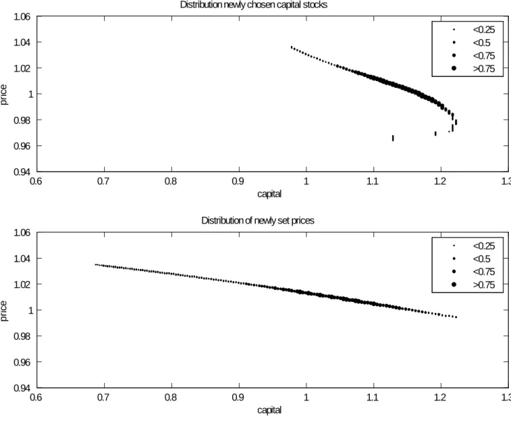
Next, we turn to the baseline calibration. The lower panel of Figure 2 illustrates the behavior of price-setters in the ergodic set.

0.6 0.7 0.8 0.9 1 1.1 1.2 1.3

0.94 0.96 0.98 1 1.02 1.04 1.06

capital

p rice

Distribution newly chosen capital stocks

<0.25

<0.5

<0.75

>0.75

0.6 0.7 0.8 0.9 1 1.1 1.2 1.3

0.94 0.96 0.98 1 1.02 1.04 1.06

capital

p rice

Distribution of newly set prices

<0.25

<0.5

<0.75

>0.75

Figure 2: Newly Chosen Capital Stocks and Prices.

Once again a clear pattern emerges. The larger a …rm’s capital stock the smaller the chosen relative price. There are, however, some important di¤erences with respect to the ‡exible price version of our model. For large enough capital stocks

10

the chosen prices are larger than their counterparts under ‡exible prices whereas the opposite is true at lower capital levels. The reason is as follows. To the extent that prices are sticky they are set in a forward-looking manner. Speci…cally, a …rm takes rationally into account that its relative price will decrease over time (due to steady state in‡ation) as long as it is not reset. In addition the …rm’s capital stock is expected to depreciate over the lifetime of the chosen price if no investment is expected to occur. Those considerations make price-setters with relatively large capital stocks choose prices that are larger than the ones that …rms with the same capital stocks would choose in the presence of ‡exible prices. If a price-setter’s capital stock is, however, smaller then it becomes more likely that an investment will take place before the price is reset. That is taken into account when price- setters form expectations regarding their marginal costs over the lifetimes of the chosen prices. This explains why newly set prices that are chosen by …rms with relatively small capital stocks are smaller than the corresponding ‡exible prices.

The upper panel of Figure 2 shows the newly chosen capital stocks. For large enough relative prices the chosen capital stock is a decreasing function of a …rm’s relative price. However, for lower relative prices this relationship becomes backward- bending. The reason is as follows. The smaller an investor’s price the likelier it is that this …rm will increase its price over the expected lifetime of the chosen capital stock. This in turn limits the size of the capital adjustment that the …rm undertakes.

Notice that the relationship between relative prices and newly chosen capital stocks is not backward-bending for larger values of relative prices. The combined e¤ect of depreciation and steady state in‡ation makes it unlikely that a …rm would choose to incur a price adjustment cost in order to decrease its price over the expected lifetime of the chosen capital stock. With those preparations we now turn to the ergodic set implied by our baseline calibration. This is shown in Figure 3.

11

0.6 0.7 0.8 0.9 1 1.1 1.2 1.3 0.94

0.96 0.98 1 1.02 1.04 1.06

capital

p rice

Distribution of (k,p) before price setting

<0.25

<0.5

<0.75

>0.75

0.6 0.7 0.8 0.9 1 1.1 1.2 1.3

0.94 0.96 0.98 1 1.02 1.04 1.06

capital

p rice

Distribution of (k,p) after price setting

<0.25

<0.5

<0.75

>0.75

Figure 3: Ergodic Set for the Baseline Model.

There are many di¤erent groups of …rms as a consequence of the interaction of pricing and investment decisions. We have already discussed the subsets of the ergodic set that correspond to newly set prices and newly chosen capital stocks.

If a …rm does not adjust neither its price nor its capital stock for the next period then that …rm moves down and to the left in the …gure due to the e¤ects of steady state in‡ation and depreciation. This is re‡ected in the lines that are parallel to the ones which correspond to the optimally chosen prices and capital stocks. Finally, the …gure also documents that price-setting occurs more frequently than investment under our baseline calibration. In fact, the lowest capital levels that are visited

12

in the ergodic set are reached because …rms …nd it optimal to let their capital depreciate over extended periods if they increase their prices from time to time in the meanwhile.

Having analyzed some important steady state properties of our model we now turn to the central question of the present paper. Does New Keynesian theory imply a quantitatively relevant monetary transmission mechanism?

3.2 The Monetary Transmission Mechanism

We consider …rst a simpli…ed version of our model which is closely related to standard textbook treatments of the monetary transmission mechanism. This will allow us to highlight important di¤erences with respect to the predictions of our baseline model. Speci…cally, it is assumed that capital is constant at the …rm level and that prices are set in a time-dependent fashion à la Calvo (1983), i.e., each …rm faces a constant and exogenous probability of getting to reoptimize its price in any given period. In order to be consistent with our baseline calibration this probability is set to 0:25. The remaining parameters are held constant at their baseline values.

13

0 5 10 15 20 -2

0 2 4 6

8 x 10

Output

0 5 10 15 20

-1 0 1 2 3

4 x 10

Inflation

0 5 10 15 20

-10 -8 -6 -4 -2 0

2 x 10

Interest Rate

0 5 10 15 20

-12 -10 -8 -6 -4 -2 0

2 x 10

Real Interest Rate

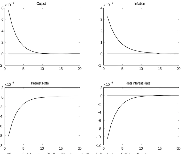
Figure 4: Monetary Policy Shocks with Fixed Capital and Calvo Pricing Figure 4 illustrates the dynamic consequences of a 100 basis point decrease in the annualized nominal interest rate. The rate of in‡ation as well as the real interest rate are also annualized and each variable is measured as the log deviation of the original variable from its steady state value. The …ndings con…rm empirical results on the monetary transmission mechanism. The standard Calvo model predicts that monetary policy shocks have strong and persistent consequences for real variables in a way that is (at least qualitatively) consistent with the empirical evidence that has been obtained using structural vector autoregressive methods. For instance, the estimates reported by Christiano et al. (2005) indicate that the maximum output

14

response to an identi…ed monetary policy shock is about 0:5 percent.

(The 95 percent con…dence interval about this point estimate is about += 0:2.) After that output is estimated to take about one and a half years to revert to its original level which is in line with the model’s prediction. The standard Calvo model is also consistent with the observed inertial behavior of in‡ation, and the maximum in‡ation response lies in the empirically plausible range.

Finally, the nominal in- terest rate takes about two quarters to return half-way to its preshock level which is another feature of the standard model that is in line with the estimates reported in Christiano et al. (2005).

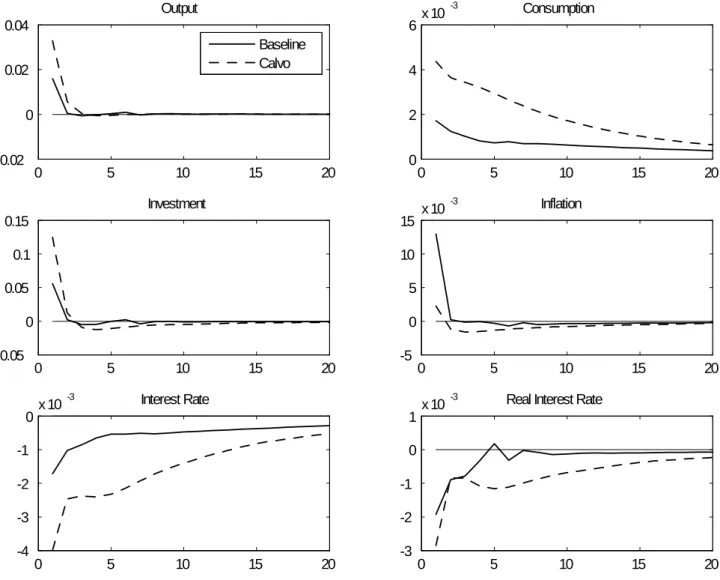
How does the monetary transmission mechanism change when the New Keyne- sian model is augmented by a micro-founded investment model? We will analyze this question under alternative assumptions regarding the price-setting of …rms. It is is natural to start with the baseline version of our model, and once again we con- sider dynamic consequences of a one hundred basis point decrease in the annualized nominal interest rate. Figure 5 illustrates our main result.

8

The maximum response is estimated to occur about six quarters after the shock. This is one reason why additional real and nominal frictions are typically added to New Keynesian models in order to increase their empirical realism. See, e.g., Christiano et al. (2005).

9

Christiano et al. (2005) estimate a maximum in‡ation response of roughly 0:2 percent which occurs about two years after the shock. (The 95 percent con…dence interval about this point estimate is about += 0:15.)

15

0 5 10 15 20 -0.02

0 0.02 0.04

Output

Baseline Calvo

0 5 10 15 20

0 2 4

6 x 10

Consumption

0 5 10 15 20

-0.05 0 0.05

0.1 0.15

Investment

0 5 10 15 20

-5 0 5 10

15 x 10

Inflation

0 5 10 15 20

-4 -3 -2 -1

0 x 10

Interest Rate

0 5 10 15 20

-3 -2 -1 0

1 x 10

Real Interest Rate

Figure 5: Monetary Policy Shocks with Lumpy Investment and Sticky Prices Under the baseline calibration monetary policy shocks do not imply empirically plausible e¤ects on real variables. Speci…cally, our model predicts an impact response of output to the monetary disturbance of about 1:5 percent, i.e., about twice as much as in the constant capital case. Moreover the presence of lumpy investment results in a dramatic reduction of the persistence in the dynamic consequences of monetary policy shocks. Finally, the relative size of the investment response to the monetary policy shock compared to the consumption response is not plausible.

Christiano et al. (2005) estimate a maximum investment response of about one percent and a maximum consumption response of roughly 0:2 percent, whereas our baseline model perdicts that the corresponding numbers are about 10 percent and

16

0:15 percent, respectively. Finally, the impact in‡ation response predicted by our baseline model is about …ve times larger than the estimated maximum response in the data. Those …ndings are in stark contrast with the empirical evidence. Figure 5 also shows that the theoretical results are even less in line with the data if Calvo pricing is assumed in the context of our lumpy investment model. In that case the impact response of output to a monetary policy shock is even stronger at a value of about 3 percent. Moreover there is still an implausible lack of persistence and both the investment and the consumption response to the monetary policy shock are unrealistically large. In a way that is consistent with the stronger impact responses of the real variables to the monetary disturbance we also …nd that the impact in‡ation response is much smaller under Calvo pricing, and better in line with the estimated maximum response.

Taken together those results suggest that the presence of a micro-founded investment decision casts doubt on the ability of sticky prices to imply a quantitatively relevant monetary transmission mechanism in the context of otherwise standard versions of the New Keynesian model.

Let us explain the economic mechanism behind our results. If investment deci- sions are conducted in an (S,s) fashion then …rms choose the timing of those decisions optimally. They therefore tend to front-load investment decisions by the time when a monetary policy shock hits the economy. In other words, …rms take rationally into account that the decrease in the real interest rate that is triggered by the monetary policy shock makes it particularly pro…table for them to invest by the time when the shock hits the economy. They therefore undertake some of the investment ac- tivity that they would have otherwise done later. This is important for two reasons.

First, the impact investment response to the shock becomes very large. Second, the distribution of …rms in the economy is altered in such a way that investment in subsequent periods becomes less likely. This explains both the enormous size of the impact response of investment to a monetary disturbance (which is driving the large output responses) and the almost complete lack of persistence in the dynamic consequences of that shock. But what is the reason behind the additional ‡exibility of in‡ation that is implied by (S,s) pricing compared to the Calvo model? Caballero and Engle (2007) argue forcefully that the answer to that question is an extensive margin e¤ect, i.e., the fact that some …rms increase their prices in response to an expansionary monetary policy shock precisely because the monetary disturbance

10

However, the fact that in‡ation reverts to its steady state level from below is another unrealistic prediction of this version of the model.

17

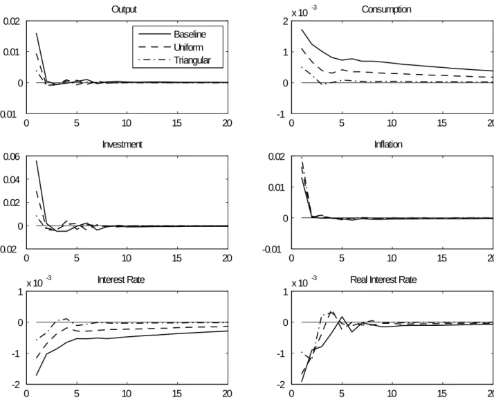
makes them reach the threshold for upward adjustment. In the Calvo model this e¤ect is absent. Those …rms which face an in…nitely large adjustment cost will not respond to the monetary disturbance and the remaining …rms would also adjust if there was no shock because this is costless for them. If the cost distribution is, however, changed in such a way that the probability mass is concentrated around intermediate values then the fraction of …rms facing costs that are too extreme to make the monetary disturbance trigger a price increase becomes smaller. In other words, the extensive margin e¤ect becomes stronger. This is the reason why in‡a- tion reacts more to a monetary policy shock if the price cost distribution is changed from Calvo to baseline, and the real consequences of monetary disturbances are consequently smaller in the baseline case. This intuition is con…rmed if we analyze the monetary transmission mechanism under two alternative forms of the price ad- justment cost density: uniform and triangular.

The results are shown in Figure 6.

11

In each case the upper bound of the support is chosen in such a way that the average frequency of price adjustment is 0:25, as in our baseline model.

18

0 5 10 15 20 -0.01

0 0.01 0.02

Output

Baseline Uniform Triangular

0 5 10 15 20

-1 0 1

2 x 10

Consumption

0 5 10 15 20

-0.02 0 0.02 0.04 0.06

Investment

0 5 10 15 20

-0.01 0 0.01 0.02

Inflation

0 5 10 15 20

-2 -1 0

1 x 10

Interest Rate

0 5 10 15 20

-2 -1 0

1 x 10

Real Interest Rate

Figure 6: Monetary Policy Shocks with Lumpy Investment and Alternative Price Adjustment Cost Distributions.

In each case the impact response of output is reduced with respect to our base- line speci…cation. Under the uniform cost density it takes a value of about 1 percent whereas the corresponding number under the triangular speci…cation is less than 0:5 percent. At the same time, however, persistence in the dynamic consequences of monetary disturbances is further reduced, the relative size of the investment re- sponse compared to the consumption response is again implausible, and the in‡ation response to the shock is unrealistically large.

19

4 Conclusion

The lumpy nature of plant-level investment is generally not taken into account in the context of monetary theory (see, e.g., Christiano et al. 2005, Woodford 2005).

We propose a generalized (S,s) pricing and investment model which is empirically more plausible along that dimension. Surprisingly, our main result shows that a quantitatively relevant monetary transmission mechanism is hard to entertain in the presence of lumpy investment. In fact, neither state-dependent pricing nor time- dependent price-setting à la Calvo can generate dynamic consequences of monetary policy shocks that are consistent with their counterpart in the data. Does this mean that an explanation for the empirical e¤ects of monetary policy shocks must be found elsewhere? Not necessarily. The results presented in the present paper hinge crucially on the (S,s) nature of the investment decisions under consideration. In fact, the monetary transmission mechanism is well and alive if pricing and investment decisions are modeled in a time-dependent fashion, as shown in Sveen and Weinke (2007).

Put into this perspective our results simply suggest that the feature of endogenous capital accumulation did not receive su¢ ciently much attention in the context of monetary models. Following up on the issues raised in the present paper will therefore be high on our research agenda. In particular, it would be interesting to see how the addition of other empirically plausible features of plant-level investment, such as time-to-build, would a¤ect the results presented here.

12

Speci…cally, Sveen and Weinke (2007) obtain the following equivalence result. If pricing and lumpy investment decisions are made in a time-dependent fashion then a convex capital adjustment cost at the …rm-level à la Woodford (2005) is observationally equivalent to its counterpart featuring lumpy investment.

20

References

Aucremanne, Luc, and Emmanuel Dhyne (2004), “How Frequently Do Prices Change?

Evidence based on the micro data underlying the Belgian CPI”, European Central Bank Working Paper No. 331.

Bachmann, Ruediger, Ricardo J. Caballero, and Eduardo R.M.A. Engel (2006),

“Aggregate Implications of Lumpy Investment: New Evidence and a DSGE Model”, NBER Working Paper 12336.

Bakhshi, Hasan, Hashmat Khan, and Barbara Rudolf (2007), “The Phillips Curve under State-Dependent Pricing”, Journal of Monetary Economics 54(8), 2321-2345.

Baudry, Laurent, Hervé Le Bihan, Patrick Sevestre, and Sylvie Tarrieu (2004),

“Price Rigidity. Evidence from the French CPI Micro-Data”, European Central Bank Working Paper No. 384.

Caballero, Ricardo J., and Eduardo R.M.A. Engel (2007), “Price Stickiness in Ss Models: New Interpretations of Old Results”, Journal of Monetary Economics 54S, 100–121.

Calvo, Guillermo (1983): “Staggered Prices in a Utility Maximizing Framework”, Journal of Monetary Economics, 12(3), 383-398.

Christiano, Lawrence J., Martin Eichenbaum, and Charles L. Evans (2005), “Nom- inal Rigidities and the Dynamic E¤ects of a Shock to Monetary Policy”, Journal of Political Economy 113(1), 1-45.

Clarida, Richard, Jordi Galí, and Mark Gertler (1999): “The Science of Monetary Policy: a New Keynesian Perspective”, Journal of Economic Literature, 37(4), 1661- 1707.

Cooper, Russell W., John C. Haltiwanger, and Laura Power (1999), “Machine Re- placement and the Business Cycle: Lumps and Bumps”, American Economic Review 89(4), 921–946.

Cooper, Russell W., and John C. Haltiwanger (2006), “On the Nature of Capital Adjustment Costs”, Review of Economic Studies 73(3), 611–633.

Dotsey, Michael, and Robert G. King (2005), “Implications of State-Dependent Pric- ing for Dynamic Macroeconomic Models”, Journal of Monetary Economics 52(1), 213-242.

21

Dotsey, Michael, Robert G. King, and Alexander L. Wolman (1999), “State-Dependent Pricing and the General Equilibrium Dynamics of Money and Output”, The Quar- terly Journal of Economics 114(2), 655-690.

Dotsey, Michael, Robert G. King, and Alexander L. Wolman (2008), “In‡ation and Real Activity with Firm-Level Productivity Shocks: A Quantitative Framework”, mimeo.

Galí, Jordi (2008), Monetary Policy, In‡ation, and the Business Cycle: An Intro- duction to the New Keynesian Framework, Princeton University Press.

Gertler, Mark and John Leahy (2008), “A Phillips Curve with an Ss Foundation”, Journal of Political Economy 116(3), 533-572.

Golosov, Mikhail, and Robert E. Lucas Jr.(2007), “Menu Costs and Phillips Curves”, Journal of Political Economy 115(2), 171-199.

Gourio, François., Anil K. Kashyap (2007), “Investment spikes: new facts and a general equilibrium exploration”, Journal of Monetary Economics 54S, 1-22.

Johnston, Michael K. (2008), “Real and Nominal Frictions within the Firm: How Lumpy Investment Matters for Price Adjustment”, mimeo, Bank of Canada.

Khan, Aubhik, and Julia K. Thomas (2008), “Idiosyncratic Shocks and the Role of Nonconvexities in Plant and Aggregate Investment Dynamics”, Econometrica 76(2), 395-436.

Krusell, Per, and Anthony A. Smith, Jr. (1998) “Income and Wealth Heterogeneity in the Macroeconomy”, Journal of Political Economy 106(5), 867-896.

Kryvtsov, Oleksiy, and Virgiliu Midrigan (2009), “Inventories, Markups, and Real Rigidities in Menu Cost Models”, Bank of Canada Working Paper 2009-6.

Midrigan, Virgiliu (2006), “Menu Costs, Multi-Product Firms, and Aggregate Fluc- tuations”, mimeo.

Nakamura, Emi, and Jon Steinsson (2008), “Five Facts About Prices: A Reevalua- tion of Menu Cost Models”, forthcoming The Quarterly Journal of Economics.

Reiter, Michael (2008), “Solving heterogeneous-agent models by projection and per- turbation”, forthcoming Journal of Economic Dynamics and Control.

Reiter, Michael (2009), “Approximate Aggregation in Heterogeneous-Agent Mod- els”, mimeo, IHS Vienna.

22

Sveen, Tommy, and Lutz Weinke (2007), “Lumpy Investment, Sticky Prices, and the Monetary Transmission Mechanism”, Journal of Monetary Economics 54S, 23-36.

Thomas, Julia K. (2002), “Is Lumpy Investment Relevant for the Business Cycle?”, Journal of Political Economy 110(3), 508-534.

Woodford, Michael (2003), Interest and Prices: Foundations of a Theory of Mone- tary Policy, Princeton University Press.

Woodford, Michael (2005), “Firm-Speci…c Capital and the New-Keynesian Phillips Curve”, International Journal of Central Banking 1(2), 1-46.

23

Appendix: Numerical Method

Each …rm, indexed by i, has two individual state variables, capital K(i) and last period’s price P (i). For the numerical solution, we discretize the state space by choosing a discrete rectangular grid in the log of K (i) and in the log of the …rm’s relative price p (i) P (i) =P . The grid is centered around the steady state values of those variables. The distance between grid points in log(K )-direction equals m log(1 ) for some integer m, such that a …rm which does not adjust its capital stock just moves m steps down the grid. The grid in log(p) is not a multiple of the in‡ation rate. If a …rm that starts at a point of the grid and does not adjust its price, then it moves down the grid by the equivalent of the in‡ation rate, and would therefore end up inbetween grid points. To stay on the discrete grid, we approximate this situation by assuming that the price jumps stochastically to one of the two neighboring grid points, such that the expected price does not change.

Solving for the steady state is a two-dimensional …xed point problem in aggregate demand Y and wage rate W . Given a guess of Y and W , we solve the …rm’s problem by the following iterative procedure:

1. Assume we have a guess of the …rm value function V (k; p). The …rm then maximizes its value, de…ned as current period pro…ts plus the discounted con- tinuation value V (k; p). Then we compute optimal choices, conditional on adjusting, as follows:

In the second part of each period, the …rm chooses next period’s k.

Choices are discrete, restricted to the points on the discrete grid. Since adjustment costs are independent of adjustment size, the optimal capital is only a function of the price set by the …rm, not its current k. The chosen capital stock enters into next period’s production.

In the …rst part of each period, the …rm chooses the price at which it sells its product in that same period. We …rst …nd the optimal p on the discrete grid; assume it is the i-th point p

. Then we assume the …rm chooses the price continuously in the range (p

; p

). Call the optimal price p , which is a function of …rm capital k, and will in general not be on the discrete grid. For the pro…t maximization, we assume that the

…rm sells at p this period, but next period the price jumps stochastically

24

to neighbouring grid points, so as to leave the expected price unchanged.

Given optimal choices, the adjustment probabilities are a function of the distribution of the adjustment costs.

2. Given a …rm policy (i.e., optimal choices of k and p), we can compute a new guess of the value function V (k; p) under the assumption that the policy is played forever. This is just a linear equation system in V .

Iterate steps 1. and 2. until convergence; this is a standard iteration in policy space, for which convergence can be proven. Given equilibrium adjustment proba- bilities, we can compute the ergodic distribution of k and p, and see whether they are consistent with the guesses of Y and W . We solve for equilibrum Y and W by a quasi-Newton method.

Having computed the steady state, we compute the dynamics, assuming (in…ni- tesimally) small shocks. We can restrict attention to the ergodic set of (k; p)-points in the steady state. With our choices for the dynamics of k and p, in…nitesimally small shocks would not move the economy away from the ergodic set. Assume the ergodic set consists of n points x

; : : : ; x

, where each x is a (k; p)-pair from the grid. At each point in time, the state vector which describes the physical state of the economy is then given by (r; (x

); (x

); : : : ; (x

)) where (x

) is the mass of …rms at point x

, and r is the nominal interest rate. The nominal interest rate is a state variable because the monetary authority attempts to smooth the interest rate over time. The vector of jump variables includes the value function at grid points V (x

) ; i = 1; : : : ; n and other aggregate variables of interest (output etc.).

We stack all the state variables plus the jump variables into the vector

. Finally, we compute a linear approximation of the dynamics of

about the steady state of those variables. If the dimension of

is not too big (up to around 2000 variables), one can solve for the exact dynamics of the linearized model using the method of Reiter (2008). Notice that this solution is linear in the aggregate variables (including the cross-sectional distribution ), but fully nonlinear in the individual variables.

We choose a grid of 400 points in p-direction and 229 points in K-direction. In the benchmark case, the ergodic set then has 7631 states. The vector therefore has around 15000 variables, and it is impossible to solve a model with this dimension on our PC. We therefore resort to model reduction techniques described in Reiter

25

(2009). The reduced model has 165 state variables and and 61 jump variables.

In the model with Calvo pricing, the ergodic set contains 20938 points. The reduced model has 185 state variables and 65 jump variables. The relative error arising from the state aggregation is in the range of 10

. The results are not sensitive to reasonable variations in the size of the grid.

13

Papers following the tradition of Krusell and Smith (1998) approximate the model using one or two state variables, which are typically some moments of the cross-sectional distribution. In our model, a precise solution cannot be otained with such a low number of variables. With 165 state variables, chosen optimally as explained in Reiter (2009), the solution is exact almost to machine precision.

26

Authors: Michael Reiter, Tommy Sveen, Lutz Weinke

Title: Lumpy Investment and State-Dependent Pricing in General Equilibrium Reihe Ökonomie / Economics Series 239

Editor: Robert M. Kunst (Econometrics)

Associate Editors: Walter Fisher (Macroeconomics), Klaus Ritzberger (Microeconomics) ISSN: 1605-7996

© 2009 by the Department of Economics and Finance, Institute for Advanced Studies (IHS),

Stumpergasse 56, A-1060 Vienna   +43 1 59991-0  Fax +43 1 59991-555  http://www.ihs.ac.at

ISSN: 1605-7996