Logic and Games SS 2009
Prof. Dr. Erich Grädel
Łukasz Kaiser, Tobias Ganzow
Mathematische Grundlagen der Informatik RWTH Aachen
c b n d
This work is licensed under:
http://creativecommons.org/licenses/by-nc-nd/3.0/de/
Dieses Werk ist lizensiert uter:
http://creativecommons.org/licenses/by-nc-nd/3.0/de/
© 2009 Mathematische Grundlagen der Informatik, RWTH Aachen.
http://www.logic.rwth-aachen.de
1 Finite Games and First-Order Logic 1
1.1 Model Checking Games for Modal Logic . . . 1
1.2 Finite Games . . . 4
1.3 Alternating Algorithms . . . 8
1.4 Model Checking Games for First-Order Logic . . . 18
2 Parity Games and Fixed-Point Logics 21 2.1 Parity Games . . . 21
2.2 Fixed-Point Logics . . . 31
2.3 Model Checking Games for Fixed-Point Logics . . . 34
3 Infinite Games 41 3.1 Topology . . . 42
3.2 Gale-Stewart Games . . . 49
3.3 Muller Games and Game Reductions . . . 58
3.4 Complexity . . . 72
4 Basic Concepts of Mathematical Game Theory 79 4.1 Games in Strategic Form . . . 79
4.2 Iterated Elimination of Dominated Strategies . . . 87
4.3 Beliefs and Rationalisability . . . 93
4.4 Games in Extensive Form . . . 96
2.1 Parity Games
In the previous section we presented model checking games for first- order logic and modal logic. These games admit only finite plays and their winning conditions are specified just by sets of positions. Winning regions in these games can be computed in linear time with respect to the size of the game graph.
However, in many computer science applications, more expressive logics like temporal logics, dynamic logics, fixed-point logics and others are needed. Model checking games for these logics admit infinite plays and their winning conditions must be specified in a more elaborate way.
As a consequence, we have to consider the theory of infinite games.
For fixed-point logics, such as LFP or the modalµ-calculus, the appropriate evaluation games are parity games. These are games of possibly infinite duration where to each position a natural number is assigned. This number is called thepriorityof the position, and the winner of an infinite play is determined according to whether the least priority seen infinitely often during the play is even or odd.
Definition 2.1. We describe a parity gameby a labelled graph G = (V,V0,V1,E,Ω)where(V,V0,V1,E)is a game graph andΩ:V→N, with |Ω(V)| finite, assigns apriorityto each position. The set V of positions may be finite or infinite, but the number of different priorities, called theindexofG, must be finite. Recall that a finite play of a game is lost by the player who gets stuck, i.e. cannot move. For infinite plays v0v1v2. . ., we have a special winning condition: If the least number appearing infinitely often in the sequenceΩ(v0)Ω(v1). . . of priorities is even, then Player 0 wins the play, otherwise Player 1 wins.
Definition 2.2. A strategy (for Playerσ) is a function f:V∗Vσ→V
such that f(v0v1. . .vn)∈vnE.
We say that a playπ=v0v1. . . isconsistentwith the strategyf of Playerσif for eachvi∈Vσit holds thatvi+1=f(vi). The strategy fis winningfor Playerσfrom (or on) a setW⊆Vif each play starting in Wthat is consistent withf is winning for Playerσ.
In general, a strategy depends on the whole history of the game.
However, in this chapter, we are interested in simple strategies that depend only on the current position.
Definition 2.3. A strategy (of Playerσ) is calledpositional(ormemoryless) if it only depends on the current position, but not on the history of the game, i.e. f(hv) = f(h′v)for allh,h′∈V∗,v∈V. We often view positional strategies simply as functionsf : V→V.
We will see that such positional strategies suffice to solve parity games by proving the following theorem.
Theorem 2.4(Forgetful Determinacy). In any parity game, the set of positions can be partitioned into two setsW0andW1such that Player 0 has a positional strategy that is winning on W0 and Player 1 has a positional strategy that is winning onW1.
Before proving the theorem, we give two general examples of positional strategies, namely attractor and trap strategies, and show how positional winning strategies on parts of the game graph may be combined to positional winning strategies on larger regions.
Remark2.5. Let f and f′be positional strategies for Playerσthat are winning on the setsW,W′, respectively. Let f+f′ be the positional strategy defined by
(f+f′)(x):=
f(x) ifx∈W f′(x) otherwise.
Then f+f′is a winning strategy onW∪W′.
Definition 2.6. LetG = (V,V0,V1,E)be a game andX⊆V. We define theattractor of X for Playerσas
Attrσ(X) ={v∈V: Playerσhas a (w.l.o.g. positional) strategy to reach some positionx∈X∪Tσ
in finitely many steps} whereTσ={v∈V1−σ:vE=∅}denotes the set of terminal positions in which Playerσhas won.
A setX⊆Vis called atrapfor Playerσif Player 1−σhas a (w.l.o.g.
positional) strategy that avoids leavingXfrom everyx∈X.
We can now turn to the proof of the Forgetful Determinacy Theo- rem.
Proof. Let G = (V,V0,V1,E,Ω) be a parity game with |Ω(V)| = m.
Without loss of generality we can assume thatΩ(V) ={0, . . . ,m−1} or Ω(V) = {1, . . . ,m}. We prove the statement by induction over
|Ω(V)|.
In the case of|Ω(V)|=1, i.e., Ω(V) ={0}orΩ(V) ={1}, the theorem clearly holds as either Player 0 or Player 1 wins every infinite play. Her opponent can only win by reaching a terminal position that does not belong to him. So we have, forΩ(V) ={σ},
W1−σ=Attr1−σ(T1−σ)and Wσ =V\W1−σ.
ComputingW1−σas the attractor ofT1−σis a simple reachability prob- lem, and thus it can be solved with a positional strategy. Concerning Wσ, it can be seen that there is a positional strategy that avoids leaving this (1−σ)-trap.
Let |Ω(v)| = m > 1. We only consider the case 0 ∈ Ω(V), i.e., Ω(V) ={0, . . . ,m−1}since otherwise we can use the same argumen- tation with switched roles of the players. We define
X1:={v∈V: Player 1 has positional winning strategy fromv},
and letgbe a positional winning strategy for Player 1 onX1.
Our goal is to provide a positional winning strategy f∗for Player 0 onV\X1, so in particular we haveW1=X1andW0=V\X1.
First of all, observe thatV\X1is a trap for Player 1. Indeed, if Player 1 could move to X1 from av∈V1\X1, thenvwould also be inX1. Thus, there exists a positionaltrap strategy f for Player 0 that guarantees to stay inV\X1.
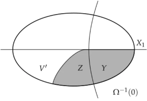
LetY=Ω−1(0)\X1,Z=Attr0(Y)and letabe anattractor strategy for Player 0 which guarantees thatY(or a terminal winning position y ∈ T0) can be reached from every z ∈ Z\Y. Moreover, letV′ = V\(X1∪Z).
The restricted gameG′ = G|V′ has less priorities thanG (since at least all positions with priority 0 have been removed). Thus, by induction hypothesis, the Forgetful Determinacy Theorem holds for G′: V′=W0′∪W1′and there exist positional winning strategies f′for Player 0 onW0′ andg′for Player 1 onW1′ inG′.
We have thatW1′=∅, as the strategy
g+g′:x7→
g(x) x∈X1
g′(x) x∈W1′
is a positional winning strategy for Player 1 onX1∪W1′. Indeed, every play consistent withg+g′either stays inW1′and is consistent withg′ or reachesX1′ and is from this point on consistent withg. ButX1, by definition, already containsallpositions from which Player 1 can win with a positional strategy, soW1′=∅.
Knowing thatW1′=∅, let f∗= f′+a+f, i.e.
f∗(x) =
f′(x) ifx∈W0′ a(x) ifx∈Z\Y
f(x) ifx∈Y
We claim that f∗ is a positional winning strategy for Player 0 from V\X1. Ifπis a play consistent with f∗, thenπstays inV\X1.
X1 V′ Z Y
Ω−1(0)
Figure 2.1.Construction of a winning strategy
Case (a):πhitsZonly finitely often. Thenπeventually stays inW0′and is consistent with f′from this point, so Player 0 winsπ.
Case (b): πhitsZinfinitely often. Thenπalso hitsYinfinitely often, which implies that priority 0 is seen infinitely often. Thus, Player 0
winsπ. q.e.d.
The following theorem is a consequence of positional determinacy.
Theorem 2.7. It can be decided in NP∩coNP whether a given position in a parity game is a winning position for Player 0.
Proof. A node vin a parity gameG = (V,V0,V1,E,Ω) is a winning position for Player σif there exists a positional strategy f :Vσ →V which is winning from positionv. It therefore suffices to show that the question whether a given strategy f :Vσ→Vis a winning strategy for Playerσfrom positionvcan be decided in polynomial time. We prove this for Player 0; the argument for Player 1 is analogous.
GivenG and f :V0→V, we obtain a reduced game graphGf = (W,F)by retaining only those moves that are consistent with f, i.e.,
F={(v,w):(v∈W∩Vσ∧w= f(v))∨ (v∈W∩V1−σ∧(v,w)∈E)}.
In this reduced game, only the opponent, Player 1, makes non- trivial moves. We call a cycle in(W,F)odd if the least priority of its
nodes is odd. Clearly, Player 0 winsGfrom positionvvia strategyf if, and only if, inGfno odd cycle and no terminal positionw∈V0is reach- able fromv. Since the reachability problem is solvable in polynomial
time, the claim follows. q.e.d.
2.1.1 Algorithms for parity games
It is an open question whether winning sets and winning strategies for parity games can be computed in polynomial time. The best algorithms known today are polynomial in the size of the game, but exponential with respect to the number of priorities. Such algorithms run in poly- nomial time when the number of priorities in the input parity game is bounded.
One way to intuitively understand an algorithm solving a parity game is to imagine a judge who watches the players playing the game.
At some point, the judge is supposed to say “Player 0 wins”, and indeed, whenever the judge does so, there should be no question that Player 0 wins. Note that we have no condition in case that Player 1 wins. We will first give a formal definition of a certain kind of judge with bounded memory, and later use this notion to construct algorithms for parity games.
Definition 2.8. A judge M = (M,m0,δ,F) for a parity game G = (V,V0,V1,E,Ω)consists of a set of statesMwith a distinguished initial state m0 ∈ M, a set of final statesF ⊆ M, and a transition function δ : V×M→ M. Note that a judge is thus formally the same as an automaton reading words over the alphabetV. But to be called a judge, two special properties must be fulfilled. Letv0v1. . . be a play ofG andm0m1. . . the corresponding sequence of states ofM, i.e.,m0is the initial state ofMandmi+1=δ(vi,mi). Then the following holds:
(1) ifv0. . . is winning for Player 0, then there is aksuch thatmk∈F, (2) if, for somek,mk∈F, then there existi<j≤ksuch thatvi=vj
and min{Ω(vi+1),Ω(vi+2), . . . ,Ω(vj)}is even.
To illustrate the second condition in the above definition, note that in the playv0v1. . . the sequencevivi+1. . .vjforms a cycle. The judge is
indeed truthful, because both players can use a positional strategy in a parity game, so if a cycle with even priority appears, then Player 0 can be declared as the winner. To capture this intuition formally, we define the following reachability game, which emerges as the product of the original gameGand the judgeM.
Definition 2.9. Let G = (V,V0,V1,E,Ω)be a parity game andM = (M,m0,δ,F) an automaton reading words overV. The reachability gameG × Mis defined as follows:
G × M= (V×M,V0×M,V1×M,E′,V×F),
where((v,m), (v′,m′))∈ E′ iff(v,v′)∈ Eandm′ =δ(v,m), and the last componentV×Fdenotes positions which are immediately winning for Player 0 (the goal of Player 0 is to reach such a position).
Note thatMin the definition above is a deterministic automaton, i.e.,δis a function. Therefore, inGand inG × Mthe players have the same choices, and thus it is possible to translate strategies betweenG andG × M. Formally, for a strategyσinGwe define the strategyσin G × Mas
σ((v0,m0)(v1,m1). . .(vn,mn)) = (σ(v0v1. . .vn),δ(vn,mn)). Conversely, given a strategyσinG × Mwe define the strategyσinG such thatσ(v0v1. . .vn) =vn+1if and only if
σ((v0,m0)(v1,m1). . .(vn,mn)) = (vn+1,mn+1),
wherem0m1. . . is the unique sequence corresponding tov0v1. . ..
Having definedG × M, we are ready to formally prove that the above definition of a judge indeed makes sense for parity games.
Theorem 2.10. Let G be a parity game and Ma judge forG. Then Player 0 winsGfromv0if and only if he winsG × Mfrom(v0,m0). Proof. (⇒) By contradiction, letσbe the winning strategy for Player 0 inG from v0, and assume that there exists a winning strategyρfor
Player 1 inG × Mfrom(v0,m0). (Note that we just used determinacy of reachability games.) Consider the unique plays
πG =v0v1. . . and πG×M= (v0,m0)(v1,m1). . .
inGandG × M, respectively, which are consistent with bothσandρ (the playπG) and withσandρ(πG×M). Observe that the positions of G appearing in both plays are indeed the same due to the wayσandρ are defined. Since Player 0 winsπG, by Property (1) in the definition of a judge there must be anmk∈ F. But this contradicts the fact that Player 1 winsπG×M.
(⇐) Letσbe a winning strategy for Player 0 inG × M, and letρ be apositionalwinning strategy for Player 1 inG. Again, we consider the unique plays
πG =v0v1. . . πG×M= (v0,m0)(v1,m1). . .
such thatπGis consistent withσandρ, andπG×Mis consistent withσ andρ. SinceπG×Mis won by Player 0, there is anmk∈Fappearing in this play.
By Property (2) in the definition of a judge, there exist two indices i<jsuch thatvi=vjand the minimum priority appearing between vi and vj is even. Let us now consider the following strategyσ′ for Player 0 inG:
σ′(w0w1. . .wn) =
σ(w0w1. . .wn) ifn<j, σ(w0w1. . .wm) otherwise,
wherem=i+ [(n−i) mod(j−i)]. Intuitively, the strategyσ′makes the same choices asσup to the(j−1)st step, and then repeats the choices ofσfrom stepsi,i+1, . . . ,j−1.
We will now show that the unique playπ′inGthat is consistent with bothσ′andρis won by Player 0. Since in the firstjstepsσ′is the same asσ, we have thatπ[n] =vnfor alln≤j. Now observe that π[j+1] =vi+1. Sinceρis positional, ifvjis a position of Player 1, then π[j+1] =vi+1, and ifvjis a position of Player 0, thenπ[j+1] =vi+1
because we definedσ′(v0. . .vj) =σ(v0. . .vi). Inductively repeating this reasoning, we get that the play π repeats the cyclevivi+1. . .vj
infinitely often, i.e.
π=v0. . .vi−1(vivi+1. . .vj−1)ω.
Thus, the minimal priority occurring infinitely often inπis the same as min{Ω(vi),Ω(vi+1), . . .Ω(vj−1)}, and thus is even. Therefore Player 0 winsπ, which contradicts the fact thatρwas a winning strategy for
Player 1. q.e.d.
The above theorem allows us, if only a judge is known, to reduce the problem of solving a parity game to the problem of solving a reachability game, which we already tackled with the Gamealgorithm.
But to make use of it, we first need to construct a judge for an input parity game.
The most naïve way to build a judge for afiniteparity gameG is to just remember, for each positionvvisited during the play, what is the minimal priority seen in the play since the last occurrence ofv. If it happens that a positionvis repeated and the minimal priority sincev last occurred is even, then the judge decides that Player 0 won the play.
It is easy to check that an automaton defined in this way indeed is a judge for any finite parity gameG, but such judge can be very big. Since for each of the|V|=n positions we need to store one of
|Ω(V)|=dcolours, the size of the judge is in the order ofO(dn). We will present a judge that is much better for smalld.
Definition 2.11. Aprogress-measuring judgeMP= (MP,m0,δP,FP)for a parity gameG = (V,V0,V1,E,Ω)is constructed as follows. Ifni =
|Ω−1(i)|is the number of positions with priorityi, then
MP={0, 1, . . . ,n0+1} × {0} × {0, 1, . . . ,n2+1} × {0} ×. . . and this product ends in· · · × {0, 1, . . . ,nm+1}if the maximal priority mis even, or in· · · × {0}if it is odd. The initial state ism0= (0, . . . , 0), and the transition functionδ(v,c)withc= (c0, 0,c2, 0, . . . ,cm)is given
by
δ(v,c) =
(c0, 0,c2, 0, . . . ,cΩ(v)+1, 0, . . . , 0) ifΩ(v)is even, (c0, 0,c2, 0, . . . ,cΩ(v)−1, 0, 0, . . . , 0) otherwise.
The setFPcontains all tuples(c0, 0,c2, . . . ,cm)in which some counter cj=nj+1 reached the maximum possible value.
The intuition behindMP is that it counts, for each even priorityp, how many positions with priority p were seen without any lower priority in between. If more thannp such positions are seen, then at least one must have been repeated, which guarantees thatMP is a judge.
Lemma 2.12. For each finite parity gameG the automatonMP con- structed above is a judge forG.
Proof. We need to show thatMPexhibits the two properties character- ising a judge:
(1) ifv0. . . is winning for Player 0, then there is aksuch thatmk∈F, (2) if, for somek,mk∈F, then there existi<j≤ksuch thatvi=vj
and min{Ω(vi+1),Ω(vi+2), . . . ,Ω(vj)}is even.
To see (1), assume that v0v1. . . is a play winning for Player 0. Let k be such an index that Ω(vk) is even, appears infinitely often in Ω(vk)Ω(vk+1). . ., and no priority higher thanΩ(vk) appears in this play suffix. Then, starting fromvk, the countercΩ(vk) will never be decremented, but it will be incremented infinitely often. Thus, for a finite gameG, it will reachnΩ(vk)+1 at some point, i.e. a state inFP.
To prove (2), letv0v1. . .vkbe such a prefix of a play that aftervk some countercpis set tonp+1 for an even priorityp. Letvi0be the last position at which this counter was 0, andvimthe subsequent positions at which it was incremented, up toinp=k. All positionsvi0,vi1, . . . ,vinp have priority p, but since there are onlynp different positions with priorityp, we get that, for somek<l,vik =vil. Nowikandilare the positions required to witness (2), because indeed the minimum priority betweenikandilispsincecpwas not reset in between. q.e.d.
For a parity gameGwith an even number of prioritiesd, the above presented judge has sizen0·n2· · ·nd, which is at most(d/2n )d/2. We get the following corollary.
Corollary 2.13. Parity games can be solved in timeO((d/2n )d/2). Notice that the algorithm using a judge has high space demand:
Since the product gameG × MP must be explicitly constructed, the space complexity of this algorithm is the same as its time complexity.
There is a method to improve the space complexity by storing the maximal counters the judgeMPuses in each position and lifting such annotations. This method is calledgame progress measuresfor parity games. We will not define it here, but the equivalence to modalµ- calculus proven in the next chapter will provide another algorithm for solving parity games with polynomial space complexity.
2.2 Fixed-Point Logics
We will define two fixed-point logics, the modalµ-calculus, Lµ, and the first-order least fixed-point logic, LFP, which extend modal logic and first-order logic, respectively, with the operators for least and greatest fixed-points.
The syntax of Lµis analogous to modal logic, with two additional rules for building least and greatest fixed-point formulas:
µX.ϕ(X)andνX.ϕ(X)
are Lµformulas ifϕ(X)is, whereXis a variable that can be used inϕ the same way as predicates are used, but mustoccur positively inϕ, i.e.
under an even number of negations (or, ifϕis in negation normal form, simply non-negated).
The syntax of LFP is analogous to first-order logic, again with two additional rules for building fixed-points, which are now syntactically more elaborate. Letϕ(T,x1,x2, . . .xn)be a LFP formula whereTstands for ann-ary relation and occurs only positively inϕ. Then both
[lfpTx.ϕ¯ (T, ¯x)](a¯)and[gfpTx.ϕ¯ (T, ¯x)](a¯)
are LFP formulas, wherea=a1. . .an.
To define the semantics of Lµand LFP, observe that each formula ϕ(X)of Lµor ϕ(T, ¯x)of LFP defines an operatorJϕ(X)K : P(V) → P(V)on statesVof a Kripke structureKandJϕ(T, ¯x)K : P(An)→ P(An) on tuples from the universe of a structureA. The operators are defined in the natural way, mapping a set (or relation) to a set or relation of all these elements, which satisfyϕwith the former set taken as argument:
Jϕ(X)K(B) ={v∈ K:K,v|=ϕ(B)}, and Jϕ(T, ¯x)K(R) ={a¯∈A:A|=ϕ(R, ¯a)}.
An argumentBis a fixed-point of an operator f if f(X) =X, and to complete the definition of the semantics, we say thatµX.ϕ(X)defines thesmallestsetBthat is a fixed-point ofJϕ(X)K, andνX.ϕ(X)defines the largestsuch set. Analogously,[lfpTx.ϕ¯ (T, ¯x)](x¯)and[gfpTx.ϕ¯ (T, ¯x)](x¯) define the smallest and largest relations being a fixed-point ofJϕ(T, ¯x)K, respectively. In a few paragraphs, we will give an alternative characteri- sation of least and greatest fixed-points, which is better tailored towards an algorithmic computation.
To justify this definition, we have to assure that all notions are well- defined, i.e., in particular, we have to show that the operators actually have fixed-points, and that least and greatest fixed-points always exist.
In fact, this relies on the monotonicity of the operators used.
Definition 2.14. An operatorFismonotoneif X⊆Y =⇒ F(X)⊆F(Y).
The operators Jϕ(X)K and Jϕ(T, ¯x)Kare monotone because we assumed that X (or T) occurs only positively in ϕ, and, except for negation, all other logical operators are monotone (the fixed-point operators as well, as we will see). Each monotone operator not only has unique least and greatest fixed-points, but these can be calculated iteratively, as stated in the following theorem.
Definition 2.15. LetAbe a set, andF:P(Ak)→ P(Ak)be a monotone
operator. We define the stagesXαof an inductive fixed-point process:
X0:=∅ Xα+1:=f(Xα)
Xλ:= [
α<λ
Xα for limit ordinalsλ.
Due to the monotonicity ofF, the sequence of stages is increasing, i.e.
Xα ⊆Xβforα < β, and hence for someγ, called theclosure ordinal, we haveXγ =Xγ+1=F(Xγ). This fixed-point is called theinductive fixed-pointand denoted byX∞.
Analogously, we can define the stages of a similar process:
X0:=Ak Xα+1:=F(Xα)
Xλ:= \
α<λXα for limit ordinalsλ.
which yields a decreasing sequence of stages Xα that leads to the inductive fixed-pointX∞:=Xγfor the smallestγsuch thatXγ=Xγ+1. Theorem 2.16(Knaster, Tarski). LetFbe a monotone operator. Then the least fixed-point lfp(F) and the greatest fixed-point gfp(F) of F exist, they are unique and correspond to the inductive fixed-points, i.e.
lfp(F) =X∞, and gfp(F) =X∞.
To understand the inductive evaluation let us consider an example.
We will evaluate the formulaµX.(P∨♦X) on the following Kripke structure:
K= ({0, . . . ,n},{(i,i+1)|i<n},{n}).
The structureKrepresents a path of lengthn+1 ending in a position marked by the predicate P. The evaluation of this least fixed-point formula starts withX0 =∅andX1 =P ={n}, and in stepi+1 all nodes having a successor inXiare added. Therefore,X2={n−1,n}, X3={n−2,n−1,n}, and in generalXk={n−k+1, . . . ,n}. Finally, Xn+1=Xn+2 ={0, . . . ,n}. As you can see, the formulaµX.(P∨♦X)
describes the set of nodes from whichP is reachable. This example shows one motivation for the study of fixed-point logics: It is possible to express transitive closures of various relations in such logics.
2.3 Model Checking Games for Fixed-Point Logics
In this section we will see that parity games are the model checking games for LFP and Lµ.
We will construct a parity gameG(A,Ψ(a¯))from a formulaΨ(x¯)∈ LFP, a structureAand a tuple ¯aby extending the FO game with the moves
[fpTx.¯ ϕ(T, ¯x)](a¯)→ϕ(T, ¯a) and
Tb¯→ϕ(T, ¯b).
We assign prioritiesΩ(ϕ(a¯))∈Nto every instantiation of a subformula ϕ(x¯). Therefore, we need to make some assumptions onΨ:
•Ψis given in negation normal form, i.e. negations occur only in front of atoms.
• Every fixed-point variable T is bound only once in a formula [fpTx.¯ ϕ(T, ¯x)].
• In a formula[fpTx.ϕ¯ (T, ¯x)]there are no other free variables besides
¯ xinϕ.
Then we can assign the priorities using the following schema:
•Ω(Ta¯)is even ifTis a gfp-variable, andΩ(Ta¯)is odd ifTis an lfp-variable.
• IfT′depends onT(i.e.Toccurs freely in[fpT′x.ϕ¯ (T,T′, ¯x)]), then Ω(Ta¯)≤Ω(T′b¯)for all ¯a, ¯b.
•Ω(ϕ(a¯))is maximal ifϕ(a¯)is not of the formTa.¯
Remark2.17. The minimal number of different priorities in the game G(A,Ψ(a¯))corresponds to the alternation depth ofΨ.
Before we provide the proof that parity games are in fact the appropriate model checking games for LFP and Lµ, we introduce the notion of anunfoldingof a parity game.
Let G = (V,V0,V1,E,Ω)be a parity game. We assume that the lowest priority m = minv∈VΩ(v) is even and that for all positions v∈ Vwith minimal priority Ω(v) =m we have a unique successor vE={s(v)}. This assumption can be easily satisfied by changing the game slightly.
We define the set T={v∈V:Ω(v) =m}
of positions with minimal priority. For any such setTwe get a modified gameG− = (V,V0,V1,E−,Ω)withE−=E\(T×V), i.e., positions in Tare rendered terminal positions.
Additionally, we define a sequence of gamesGα= (V,V0α,V1α,E−,Ω) that only differ in the assignment of the terminal positions inT to the players. For this purpose, we use a sequence of disjoint pairs of sets T0α and T1α such that each pair partitions the set T, and let Vσα= (Vσ\T)∪T1−σα , i.e., Playerσwins at final positionsv∈Tσα. The sequence of partitions is inductively defined depending on the winning regions of the players in the gamesGαas follows:
•T00:=T,
•T0α+1:={v∈T:s(v)∈W0α}for any ordinalα,
•T0λ:=Sα<λT0αifλis a limit ordinal,
•T1α=T\T0αfor any ordinalα.
We have
•W00⊇W01⊇W02⊇. . .⊇W0α⊇W0α+1. . .
•W10⊆W11⊆W12⊆. . .⊆W1α⊆W1α+1. . .
So there exists an ordinalα≤ |V|such thatW0α =W0α+1 =W0∞and W1α=W1α+1=W1∞.
Lemma 2.18(Unfolding Lemma).
W0=W0∞ and W1=W1∞.
Proof. Letαbe such thatW0∞=W0αand letfαbe a positional winning
strategy for Player 0 fromW0αinG. Define:
f : V0→V : v7→
fα(v) ifv∈V0\T, s(v) ifv∈V0∩T.
A playπconsistent with f that starts inW0∞never leavesW0∞:
• Ifπ(i) ∈W0∞\T, thenπ(i+1) = fα(π(i)) ∈W0α =W0∞(fαis a winning strategy inGα).
• Ifπ(i) ∈ W0∞∩T =W0α∩T =W0α+1∩T, thenπ(i) ∈ T0α+1, i.e.
π(i)is a terminal position inGαfrom which Player 0 wins, so by the definition ofT0α+1we haveπ(i+1) =s(v)∈W0α=W0∞. Thus, we can conclude that Player 0 winsπ:
• IfπhitsTonly finitely often, then from some point onwardsπis consistent with fαand stays inW0αwhich results in a winning play for Player 0.
• Otherwise,π(i) ∈Tfor infinitely manyi. Since we hadΩ(t) = m ≤Ω(v)for allv∈ V,t ∈ T, the lowest priority seen infinitely often ism, which we have assumed to be even, so Player 0 winsπ.
Forv∈ W1∞, we define ρ(v) =min{β : v ∈W1β}and let gβ be a positional winning strategy for Player 1 onW1βinGβ. We define a positional strategygof Player 1 inG∞by:
g:V1→V, v7→
gρ(v)(v) ifv∈W1∞\T∩V1
s(v) ifv∈T∩V1 arbitrary otherwise
Letπ=π(0)π(1). . . be a play consistent withgandπ(0)∈W1∞. Claim2.19. Letπ(i)∈W1∞. Then
(1)π(i+1)∈W1∞, (2)ρ(π(i+1))≤ρ(π(i))
(3)π(i)∈T⇒ρ(π(i+1))<ρ(π(i)).
Proof. Case (1): π(i) ∈ W1∞\T, ρ(π(i)) = β (so π(i) ∈ W1β). We have π(i+1) = g(π(i)) = gβ(π(i)), soπ(i+1) ∈ W1β ⊆ W1∞ and ρ(π(i+1))≤β=ρ(π(i)).
Case (2): π(i) ∈ W1∞∩T, ρ(π(i)) = β. Then we have π(i) ∈ W1∞, β = γ+1 for some ordinal γ, and π(i+1) = s(π(i)) ∈ W1γ, so π(i+1)∈W1∞andρ(π(i+1))≤γ<β=ρ(π(i)). q.e.d.
As there is no infinite descending chain of ordinals, there exists an ordinalβsuch thatρ(π(i)) =ρ(π(k)) =βfor alli≥k, which means thatπ(i) ̸∈Tfor alli ≥k. Asπ(k)π(k+1). . . is consistent withgβ andπ(k)∈W1β, soπis won by Player 1.
Therefore we have shown that Player 0 has a winning strategy from all vertices inW0∞and Player 1 has a winning strategy from all vertices in W1∞. AsV = W0∞∪W1∞, this shows thatW0 = W0∞ and
W1=W1∞. q.e.d.
We can now give the proof that parity games are indeed appropriate model checking games for LFP and Lµ.
Theorem 2.20. IfA|=Ψ(a¯), then Player 0 has a winning strategy in the gameG(A,Ψ(a¯))starting at positionΨ(a¯).
Proof. By structural induction overΨ(a¯). We will only consider the inter- esting casesΨ(a¯) = [gfpTx.ϕ¯ (T, ¯x)](a¯)andΨ(a¯) = [lfpTx.ϕ¯ (T, ¯x)](a¯).
LetΨ(a¯) = [gfpTx.¯ϕ(T, ¯x)](a¯). In the gameG(A,Ψ(a¯)), the posi- tionsTb¯ have priority 0. Every such position has a unique successor ϕ(T, ¯b), so the unfoldingsGα(A,Ψ(a¯))are well defined.
Let us take the chain of steps of the gfp-induction ofϕ(x¯)onA.
X0⊇X1⊇. . .⊇Xα⊇Xα+1⊇. . . We have
A|=Ψ(a¯) ⇔ a¯∈gfp(ϕA)
⇔ a¯∈Xαfor all ordinalsα
⇔ a¯∈Xα+1for all ordinalsα
⇔ (A,Xα)|=ϕ(a¯)for all ordinalsα.
Induction hypothesis: For everyX⊂Ak
(A,X)|=ϕ(b¯) iff Player 0 has a winning strategy in G((A,xα),ϕ(a¯))fromϕ(a¯).
We show: If Player 0 has a winning strategy inG((A,xα),ϕ(a¯))starting at position ϕ(a¯), then Player 0 has a winning strategy inGα(A,Ψ(a¯)) starting at positionϕ(a¯).
By the unfolding lemma, the second statement is true for all or- dinals αif and only if Player 0 has a winning strategy inG(A,Ψ(a¯) starting atϕ(a¯).
Asϕ(a¯)is the only successor ofΨ(a¯) = [gfpTx.ϕ¯ (T, ¯x)](a¯), this holds exactly if Player 0 has a winning strategy inG(A,Ψ(a¯))starting atΨ(a¯).
It remains to show that Player 0 has indeed a winning strategy in the gameG((A,xα),ϕ(a¯))starting at the positionϕ(a¯).
There are few differences betweenG((A,xα),ϕ(a¯))and the unfold- ingGα(A,Ψ(a¯)):
• InGα(A,Ψ(a¯)), there is an additional positionΨ(a¯), but this posi- tion is not reachable.
• The assignment of the atomic propositionsTb:¯
– Player 0 wins at positionT¯binG((A,xα),ϕ(a¯))if and only if b¯∈Xα.
– Player 0 wins at position Tb¯ in Gα(A,Ψ(a¯)) if and only if Tb¯∈T0α.
So we need to show using an induction overαthat b¯∈Xα iff Tb¯∈T0α.
Base caseα=0:X0=AkandTα0=T={Tb¯ : ¯b∈Ak}.
Induction stepα=γ+1: Then ¯b∈Xα=Xα+1if and only if(A,Xγ)|= ϕ(b¯), which in turn holds if Player 0 wins G((A,Xγ),ϕ(b¯))starting at ϕ(b¯). By induction hypothesis, this holds if and only if Player 0 wins the unfoldingGγ(A,Ψ(a¯))starting atϕ(b¯) =s(Tb¯)if and only if Tb¯ ∈T0γ+1=T0α.
Induction step withαbeing a limit ordinal:We have that ¯b∈Xαif ¯b∈Xγ for all ordinalsγ<α, which holds, by induction hypothesis, if and only ifTb¯ ∈T0γfor allγ<α, which is equivalent toTb¯ ∈T0α.
The proof forΨ(a¯) = [gfpTx.ϕ¯ (T, ¯x)](a¯)is analogous. q.e.d.
2.3.1 Defining Winning Regions in Parity Games
To conclude, we consider the converse question—whether winning regions in a parity game can be defined in fixed-point logic—and show that, given an appropriate representation of parity games as structures, winning regions are definable in theµ-calculus.
To represent a parity game G = (V,V0,V1,E,Ω) with priori- ties Ω(V) = {0, 1, . . . ,d−1}, we use the Kripke structure KG = (V,V0,V1,E,P0, . . . ,Pd−1). The universe and edge relation of this Kripke structure are the same as in the parity game, and so are the predicates V0 and V1 assigning positions to players. The only difference is in the predicatesPj, which are used to explicitly represent positions with priorityj, i.e. we definePj={v∈V:Ω(v) =j}.
Given the above representation, theµ-calculus formula ϕWind =νX0.µX1.νX2. . . .λXd−1
d−1_ j=0
(V0∧Pj∧♦Xj)∨
(V1∧Pj∧Xj), whereλ = νifdis odd, andλ =µotherwise, defines the winning region of Player 0 in the sense of the following theorem.
Theorem 2.21. KG,v |= ϕWind if and only if Player 0 has a winning strategy fromv0inG.
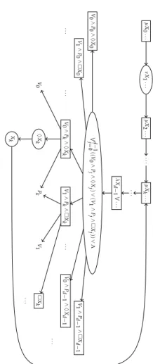
Proof (Idea). The model checking game forϕWind onKGis essentially the same as the gameGitself, up to some negligible modifications:
• eliminate moves after which the opponent wins in at most two steps (e.g. Verifier would never move to a position(V0∧Pj∧♦Xj,v) ifvwas not a vertex of Player 0 or did not have priorityj),
• contract sequences of trivial moves and remove the intermediate positions.
A schematic view of a model checking game forϕWind is sketched in
µX0...νX1...µX2......µXk...
...
λXd−1 W... Wd−1j=0((V0∧Pj∧♦Xj)∨(V1∧Pj∧Xj))∨ΛV0∧P0∧♦X0 V1∧P0∧X0...V0∧Pk∧♦XkV1∧Pk∧Xk...V0∧Pd−1∧♦Xd−1 V1∧Pd−1∧Xd−1
V0♦XkPkV1Xk
Xk ...
...
...
Figure2.2.PartofamodelcheckinggameforϕWind.