Theoretical Analysis and Large-Eddy Simulations of the Propagation of Land-Surface Heterogeneity in the Atmosphere

Theoretical Analysis and Large-Eddy Simulations of the Propagation of Land-Surface Heterogeneity in

the Atmosphere

Inaugural-Dissertation zur

Erlangung des Doktorgrades

der Mathematisch-Naturwissenschaftlichen Fakultät der Universität zu Köln

vorgelegt von

Michael Hintz aus Radevormwald

Köln 2016

Gutachter:

1. Berichterstatter (Betreuer): Prof. Dr. Yaping Shao

2. Berichterstatter: Prof. Dr. Stefan Kollet

Tag der mündlichen Prüfung: 1. Dezember 2015

To my Father

Zusammenfassung

Die vorliegende Arbeit beschäftigt sich mit der Frage wie man Bodenheteroge- nitäten quantifizieren kann und wie sie sich auf die atmosphärische Grenzschicht auswirken. In der Grenzschicht werden Energie und Masse hauptsächlich durch große Wirbel transportiert. Deswegen ist es wichtig zu verstehen, welche Auswir- kungen Heterogenitäten auf diese Wirbel haben. Da diese Wirbel eine komplexe Struktur besitzen und auf einer großen Bandbreite von Skalen variieren, ist es sehr aufwendig Informationen über sie durch Messungen zu erhalten. Hoch aufgelöste Modelle bieten hier eine Alternative. In dieser Studie, wird ein zwischen Boden und Atmosphäre gekoppeltes großes Wirbel Model verwendet. Dieses ist in der Lage die großen Wirbel explizit aufzulösen und kann so benutzt werden, die auf- tretenden Fragestellungen zu beantworten.

In dieser Arbeit wird eine kurze Einführung in die Theorie der großen Wirbel Simulationen gegeben. Außerdem gibt sie einen Überblick über einige der Ver- fahren welche benutzt werden um Heterogenitäten zu quantifizieren. Die in die- ser Arbeit entwickelte Methode, die sogenannte Entropiespektrumsmethode, wel- che zur Quantifizierung verwendet wird, wir anschließend erklärt. Bei dieser Me- thode werden die räumlich verteilten Daten (sowohl atmosphärische Größen als auch Landoberflächenparameter) mit Hilfe der Wavelettransformation in hoch- und tiefpassgefilterten Anteile zerlegt. Für jeden einzelnen Anteil wird anschlie- ßend die Shannon Entropie berechnet. Es wird außerdem gezeigt, wie man mit Hilfe der Entropiespektrumsmethode die dominante Skala einer Heterogenität be- stimmen kann.

Um zu zeigen, welchen Einfluss unterschiedliche Heterogenitäten auf die atmo-

sphärische Grenzschicht haben, werden neun verschiedene Landnutzungsmuster

untersucht. Für jedes Muster werden Simulationen mit dem gekoppelten großen

Wirbelmodel durchgeführt. Die Simulationsergebnisse werden mit der Entropie-

spektrumsmethode untersucht. Dies geschieht für die potentielle Temperatur, das

Wasserdampfmischungsverhältnis, sowie für den sensiblen und den latenten Wär-

mefluss. Die Untersuchung wird sowohl für instantane und als auch für zeitlich

gemittelte Werte durchgeführt. Die Anwendung der Methode auf die Modeller-

gebnisse dient außerdem der Untersuchung ab welcher Höhe der Einfluss der He-

terogenität vernachlässigbar ist. Die Ergebnisse zeigen, dass das Verhalten des

Entropiespektrums davon abhängt, welche Größe untersucht wird. Dies läßt ver-

muten, dass die atmosphärische Antwort auf Landoberflächenheterogenität sehr

komplex ist. Des Weiteren zeigt sich, dass für die gewählten Heterogenitäten die

instantanen Werte weniger Aussagekraft darüber besitzen, ab wann der Einfluss

des Bodens vernachlässigbar ist, als die zeitlich gemittelten Werte. Die Analyse

Größe als von der verwendeten Landnutzung. Die Ergebnisse zeigen, dass für die untersuchten Daten der Einfluss der Heterogenität oberhalb von 400 m für die gemittelte potentielle Temperatur und das gemittelte Wasserdampfmischungsver- hältnis; oberhalb von 260 m für den gemittelten sensiblen Wärmefluss; und für variierende Höhen für den gemittelten latenten Wärmefluss, vernachlässigbar ist.

Ab dieser Höhe überwiegt das Eigenmuster, welches durch die Selbstorganisation der Turbulenz erzeugt wird, den Einfluss der Landoberflächenheterogenität.

Ein Vergleich der Entropiespektrumsmethode, welche den Informationsaspekt der

Heterogenität beschreibt, mit statischen Methoden, welche die Struktur beschrei-

ben, zeigt für homogene und zufällige Muster gute Übereinstimmung. Für eine

real existierende Heterogenität ist die Entropiespektrumsmethode überlegen. Die

Entropiespektrumsmethode zeigt außerdem, welchen Einfluss die Auflösung der

Heterogenität auf die Atmosphäre hat. Dieser ist wieder abhängig von der betrach-

teten physikalischen Größe und ob die zugrunde liegenden Heterogenität korre-

liert oder zufällig angeordnet ist.

Abstract

This thesis deals with the questions how land-surface heterogeneity can be quanti- fied and how it can influence the atmospheric boundary layer. In this layer energy and mass are mainly transported by large eddies and therefore, it is important to understand how they are affected by the land-surface heterogeneities. Since large eddies have complex structures, which vary on a wide range of scales, it is highly demanding to obtain knowledge about them via measurements. High-resolution models offer an alternative. In this study, an atmosphere and land-surface coupled large-eddy simulation (LES) model, which explicitly resolves the large eddies, is used to address the concerned questions.

In this thesis a short introduction to the theory of LES is given, followed by an outline of some approaches for heterogeneity quantification. The method devel- oped in this study for the quantification, namely, the entropy spectrum method, is then explained. In this method, the spatially-distributed data (of atmosphere and land-surface quantities and parameters) are decomposed into low- and high-pass filtered parts via wavelet transformation. For each part, the Shannon entropy is calculated. It is elaborated how to obtain from the entropy spectrum the dominant scale of the heterogeneity.

In order to investigate how land-surface heterogeneity influences the atmospheric

boundary layer, nine different land-use patterns are designed. Simulations with

the atmosphere and land-surface coupled LES model are carried out for each of

these patterns. The simulation results, including potential temperature, water-

vapor-mixing ratio, sensible and latent heat fluxes, are analyzed with the entropy

spectrum method. The analysis is done for instantaneous as well for temporally

averaged values and is found useful for identifying the height above which the

influence of land-surface heterogeneity is negligible. The results show that the

entropy spectra differ for different atmospheric variables, suggesting that the re-

sponse of the atmosphere to land-surface heterogeneity is rather complex. In ad-

dition, it is shown that for a given land-surface pattern, the instantaneous values

are less helpful to answer the question above which height the influence of the het-

erogeneity is negligible, than the temporally averaged values. The analysis with

the temporally averaged values shows larger differences between the spectra of

different parameters than between the spectra of the same parameter for different

heterogeneities. From the results, it is concluded that for the cases investigated,

the influence of the heterogeneity is negligible above 400 m height for the aver-

aged values of potential temperature and water-vapor-mixing ratio; 260 m for the

averaged sensible heat flux (of some experiments); and varying heights for the av-

eraged latent heat flux. Above these heights it is concluded that the Eigen-pattern

land-surface heterogeneity.

A comparison of entropy, which describes the information aspect of heterogene-

ity, with statistical methods, which describe the structure aspect of heterogeneity,

shows a good agreement for homogeneous and random patterns. For a real exist-

ing heterogeneity, the entropy spectrum method is superior. Moreover, the entropy

spectrum method shows how the resolution of heterogeneity influences the atmo-

sphere. This influence is dependent on the investigated physical variable and if

the investigated heterogeneity is correlated or random.

Contents

1 Introduction 1

2 Turbulent Flows in the Atmosphere 7

2.1 Governing Equations . . . . 7

2.2 The Closure Problem . . . . 14

2.3 Monin-Obukhov Similarity Theory . . . . 15

2.4 Large-Eddy Simulation . . . . 19

3 Existing Methods for Heterogeneity Quantification 31 3.1 Taylor Diagram . . . . 32

3.2 Variogram . . . . 34

3.3 Power Spectrum . . . . 35

3.4 Probability Density Function . . . . 35

3.5 Wavelet Transformation . . . . 36

3.6 Entropy . . . . 38

3.7 Entropy Spectrum . . . . 46

4 Methodology 51 4.1 Estimation of the Dominant Scale . . . . 51

4.2 Data and Model Setup . . . . 55

4.3 Entropy Analysis of the Land Use Patterns . . . . 56

5 Results 65 5.1 Normalization . . . . 65

5.2 Responses to a Homogeneous Pattern . . . . 67

5.3 Instantaneous Responses . . . . 69

5.5 The Influence of Resolution . . . . 81 5.6 Comparison to other Methods . . . . 86

6 Conclusion 95

List of Figures

Figure 2.1 LES-ALM configuration . . . . 26

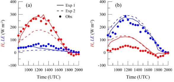
Figure 2.2 Comparison of the LES-ALM with measurements . . . . . 28

Figure 3.1 Geometric relationship between R, E

, σ

and σ

. . . . . 33

Figure 3.2 Example of a Taylor diagram . . . . 34

Figure 3.3 Example of a homogeneous and a heterogeneous pattern . . 36

Figure 3.4 Patterns to illustrate the problem of entropy . . . . 44

Figure 3.5 Illustration of the entropy spectrum method . . . . 47

Figure 3.6 Illustration of the reference entropy spectrum . . . . 48

Figure 4.1 High-resolution random data with the same PDF . . . . 52

Figure 4.2 Entropy spectrum to distinguish pattern with same PDF . . 52

Figure 4.3 Input data for the nine numerical experiments . . . . 57

Figure 4.4 Entropy spectra for the model input . . . . 58

Figure 5.1 Temperature pattern for a homogeneous land surface . . . . 67

Figure 5.2 Water-vapor-mixing-ratio for a homogeneous land surface . 68 Figure 5.3 Entropy spectrum of the instantaneous values of Θ, q, H, LE 69 Figure 5.4 Entropy spectrum of the averaged values of Θ, q, H, LE . 73 Figure 5.5 Scale of S

for the averaged value of Θ . . . . 75

Figure 5.6 Scale of S

for the averaged value of q . . . . 77

Figure 5.7 Scale of S

for the averaged value of H . . . . 79

Figure 5.8 Scale of S

for the averaged value of LE . . . . 81

Figure 5.9 Influence of resolution of correlated land use patterns . . . 83

Figure 5.10 Influence of resolution of uncorrelated land use patterns . . 85

Figure 5.11 Example Taylor diagram of model results . . . . 87

Figure 5.12 Comparison between entropy, R and E

for experiment (a) 89

Figure 5.14 Comparison between entropy, R and E

for experiment (d) 93

List of Tables

Table 2.1 Illustration of the closure problem . . . . 14 Table 4.1 Model setup and comparison with Shao et al. [2013] . . . . 55 Table 4.2 Conversion between land use types and albedo values . . . . 56 Table 4.3 Entropy of the different land use inputs and entropy values

of averaged Θ, q, H and LE at the surface . . . . 59

1 Introduction

Modern weather forecasting and climate projection rely primarily on numerical models. To improve these models, it is necessary to better understand the physical processes which influence the weather and climate system and to better repre- sent them in the models. Of particular interest to this study are the atmosphere and land-surface interactions over heterogeneous areas that determine the model lower boundary conditions. In recent years, the resolution of weather and climate models has significantly increased, from 10 km to 1 km in the case of numer- ical weather forecast and from 100 to 10 km in the case of climate projection.

However, the resolutions are still insufficient to resolve all relevant processes, and the unresolved processes have to be parametrized. There are two types of parametrization: the first type involves the representation of the interactions be- tween the model-resolved (grid-scale) and model-unresolved (sub-grid-scale) pro- cesses, known also as the closure problem, and the second type involves the rep- resentation of the interactions between the atmosphere and the other components of the weather/climate system, e.g. between the atmosphere and the land surface, i.e., the parametrization of the model boundary conditions.

An effective transport mechanism in the atmospheric boundary layer is the con-

vection by large eddies, and hence to investigate the atmosphere and land-surface

interactions on the large-eddy scale is of particular importance. As large eddies

span over a wide range of scales, high-resolution data both in space and time for

variables like temperature, humidity and wind speed are required for their charac-

terization. It is highly demanding to obtain such data via measurements, although

concerted effort has been made over the years in field campaigns. The difficulty

is in particular to obtain suitable data sets for the characterization the atmosphere

and land-surface coupled system over heterogeneous land surfaces. As an alter- native, large-eddy simulations (LES) (cf. Section 2.4) can be used to generate high-resolution synthetic data for the purpose. In recent years, LES models have been substantially improved for studying atmosphere and land surface interac- tions.

Most weather and climate models assume a spatially homogeneous land surface on the sub-grid scale. This is reflected in the fact, that the parametrization of surface fluxes relies on the Monin-Obukhov Similarity Theory (cf. Section 2.3).

This assumption may be in general too simplistic. Studies so far have demon- strated that land-surface heterogeneity on the grid scale as well as on the subgrid scale are both important to the exchanges of energy and mass between the atmo- sphere and the land surface (e.g. Hechtel et al. [1990]; Mahrt [2000]; Heinemann and Kerschgens [2005]).

On the subgrid scale, studies (e.g. Avissar and Pielke [1989], Shao et al. [2001]) identified the "aggregation effects" and "dynamic effects" of heterogeneity. The aggregation effect occurs because the fluxes estimated using spatially averaged state variables differ from spatially averaged fluxes. This is a consequence of the non-linear relationships between the fluxes and the state variables. Dynamic effects occur because land-surface heterogeneity can generate sub-grid-scale mo- tions, which contribute to the exchange processes, but are not accounted for in the parametrization.

A widely used method for the treatment of land-surface heterogeneity in land- surface schemes is the "mosaic" method (Avissar and Pielke [1989]; Koster and Suarez [1992]) in which land-surface cells with the same properties are grouped into patches for which the fluxes are then computed. This method recognizes the importance of the land-surface properties, but neglects the spatial variations of the atmospheric variables and the dynamic effects associated with land-surface het- erogeneity.

More recently, a downscaling technique has been proposed by Schomburg et al.

[2010], which takes the effect of land-surface heterogeneity on the atmosphere into account. However, this technique is mainly a statistical manipulation of the data and is not a sufficient representation of the dynamic effects. The resolution is an important issue of modeling the atmosphere. The modeling of the land-surface itself on the grid-resolved scale is difficult. In addition, if land-surface hetero- geneity lies on a sub-grid-scale of the model, it is difficult to resolve the effect of land-surface heterogeneity on the grid-scale.

Mahrt [2000] gave an overview of the blending height concept. He viewed the blending height as a scaling depth that describes the decrease of the influence of surface heterogeneity with height. The author was aware of the fact that the blend- ing height is not a level where the influence of the surface heterogeneity suddenly and completely vanishes, but a height where the influence of the surface hetero- geneity decreases below a threshold. This concept is useful for some applications.

However, to find a universal threshold value is in general difficult. In addition, for most of the blending height concepts there is only one heterogeneity scale.

The problem how to obtain this heterogeneity scale, leads to the problem how to quantify it.

One current research goal is to parametrize heterogeneous land-surface processes in weather and climate models. In order to achieve this goal several steps are necessary: (1) development of an LES model to obtain high-resolution data; (2) development of suitable decompositions of land-surface heterogeneity; (3) quan- tification of land-surface heterogeneity; (4) investigation of the propagation of land-surface heterogeneity in the atmospheric boundary layer; (5) describing the heterogeneity with only a few parameters in order to reconstruct land-surface het- erogeneity; and (6) parametrization of land-surface heterogeneity in weather and climate models.

Point (1), the development of an LES model, has already been done by Shao et al.

[2013]. With this model it is possible to obtain the high-resolution data needed to

investigate the structure of the atmospheric boundary. The emphasis of this thesis

are the points (2) - (4). Possible decomposition methods are the Fourier transfor-

mation and the wavelet transformation (Morlet et al. [1982]; Daubechies [1990]).

Both of them have been used in various applications (Bacry et al. [1993]; Briggs and Levine [1997]). In this thesis the wavelet transformation is used, because it keeps the prominent features of the heterogeneity unchanged.

For the quantification of land-surface heterogeneity many approaches are pos- sible. Which one should be used depends on the scientific question. Garrigues et al. [2006] gave an overview of the methods used for the quantification of spatial heterogeneity. These include the autocorrelation (Ford [1976]), fractals (Mandel- brot [1983]), the local variance (Woodcock and Strahler [1987]), the variogram (Curran [1988]), spectral methods (Hough [1989]), the hierarchical decomposi- tion (Woodcock and Harward [1992]) or the probability density function (PDF) (Giorgi [1997]). Other studies (e.g. Andraud et al. [1998]; Van Siclen [1997];

Fjellstad et al. [2001]), make use of the information entropy (Shannon [1948]).

Some studies combine the variogram with wavelet transformation (Gloaguen and Dimitrakopoulos [2009]), while others use empirical orthogonal functions, cf.

Hannachi et al. [2007] for a review. However, in this thesis the entropy spec- trum method is independently developed and used, which is a combination of the Shannon entropy and wavelet transformation. In some earlier studies (Labat [2005]; Brunsell et al. [2008, 2011]; Brunsell and Anderson [2011]), aspects of the method proposed in this thesis have been used.

Another focus of this study is on point (4), i.e., the investigation of the propaga-

tion of land-surface heterogeneity in the atmospheric boundary layer. This point

has been studied to some extent by Courault et al. [2007]; Huang and Margulis

[2009] and Shao et al. [2013]. In this thesis, the focus lies on the response of at-

mospheric quantities such as temperature, moisture, sensible and latent heat fluxes

to land-surface heterogeneity. To this end, atmosphere and land-surface coupled

large-eddy simulations are carried and the results are analyzed with the entropy

spectrum method.

In this thesis, the following two research questions are examined:

1. How to quantify land-surface heterogeneity?

2. Above which height is the influence of land-surface heterogeneity negligible?

The answer to the first question is the quantification of land-surface heterogeneity with the entropy spectrum method. The second question is answered by investi- gating the entropy spectra at different heights of the simulation results obtained with a coupled LES model.

The outline of the thesis is as follows. In Chapter 2 the basic theory for LES

is given. In Chapter 3 a brief review of some existing methods for heterogeneity

quantification is given. In Chapter 4 the improvements to the entropy spectrum

and the input data and the model setup are described. In addition, an analysis

of the different land-use patterns with the entropy spectrum method is shown. In

Chapter 5 the results from the LES model are shown in order to investigate the

atmospheric response to the different land use patterns. As an example the pat-

terns and spectra for a homogeneous land-use pattern are shown. Afterwards, the

atmospheric responses on different time scales to land-surface heterogeneity are

investigated. It is also dealt with the question how the resolution of the land-use

patterns influences the entropy spectra. In addition, a comparison of the entropy

spectrum method with other methods is done. The thesis is closed with a conclu-

sion.

2 Turbulent Flows in the Atmosphere

2.1 Governing Equations

In order to understand the results of the present thesis, it is necessary to first ex- plain the model with which they are obtained. The large eddy version of the WRF (Weather Research and Forecast) model is used for this study. WRF, a numerical weather prediction model, solves a set of equations for the atmospheric motion, known as the governing equation, which consists of the continuity equation, the equation of motion, the conservation of moisture, the conservation of energy and the equation of state. As the governing equations are coupled and contain non- linear terms, they must be solved numerically.

The differences between the models for atmospheric motions on different scales

are diminishing. A numerical weather prediction (NWP) model can be used today

for LES, if the model resolution is sufficiently high. Models, which can explicitly

resolve the large-eddy scale turbulent processes in the atmosphere, i.e., the model

resolution corresponds to the inertial sub-range of the turbulence, are called LES

models. In order to understand how an LES model works, it is necessary to under-

stand the governing equations for atmospheric turbulent flows and to know how

they are solved. In this Chapter, the governing equations are presented, followed

by an illustration of the averaging method used in most NWP models. The closure

problem together with the assumption of spatial homogeneity, which is made in

most NWP/climate models, is then discussed. After the discussion of these basics,

the technique of LES is explained.

2.1.1 Continuity Equation

The conservation of mass states that the temporal change of density ρ in a certain volume is determined by the divergence of the mass flux ρu,

∂ρ

∂t + ∇ · (ρu) = 0. (2.1)

Where u is velocity and ∇ is the Nabla operator. This equation can be written in its component form using the summation convention that a summation goes over double indices in one term,

∂ρ

∂t + ∂ρu

∂x

= 0. (2.2)

For velocities much smaller than the speed of sound, the air can be assumed as an incompressible fluid and Equation (2.2) reduces to

∂u

∂x

= 0, (2.3)

which is known as the incompressibility approximation. For this kind of fluids, ρ does not depend on position x or time t.

2.1.2 Equation of Motion

The derivation of the equation of motion starts with Newton’s second law

F = ma, i.e., force equals mass times acceleration. Mainly three external forces act on an air parcel in the atmosphere. These forces are the gravitational force, the Coriolis force and the pressure gradient force. The gravitational force is

F

= −mg, with g = (0, 0, 9.81 m/s

)

. The Coriolis force is F

= 2mu × Ω, with u the velocity of the particle and Ω = (0, ω cos φ, ω sin φ)

the angular velocity vector, with the latitude φ and ω the angular velocity of the earth. The pressure gradient force is F

= −

∇p, with the density ρ and the pressure p.

With this, it follows the equations of motion F = ma = m du

dt = −2mΩ × u − mg − m

ρ ∇p. (2.4)

2.1. Governing Equations If the total time derivative is decomposed and divided by the mass, the results are the Euler equations

∂u

∂t + u∇ · u = −2Ω × u − g − 1

ρ ∇p. (2.5)

In the following the so-called flux form of the Euler equations will be derived. For a quantity a given in advection form, i.e. u

j

, the flux form can be obtained by adding the continuity equation multiplied by a.

u

∂a

∂x

+ a ∂u

∂x

|{z}

=0

= ∂ (au

)

∂x

. (2.6)

If the advection form of Equation (2.5) is written in its components, it follows that

∂u

∂t + u

∂u

∂x

= ε

f

u

− δ

g − 1 ρ

∂p

∂x

. (2.7)

With ε

being the Levi-Civita-Pseudo-Tensor, δ

the Kronecker delta and where f

= 2ω sin φ denotes the Coriolis parameter. From Equation (2.7) follows the Euler equations in flux form

∂u

∂t + ∂ (u

u

)

∂x

= ε

f

u

− δ

g − 1 ρ

∂p

∂x

. (2.8)

The Euler Equations are valid for a fluid without friction. If the viscous stress for an incompressible fluid

∆u (Landau and Lifshitz [1987];Prager [2004]), where µ is the viscosity, is added to Equation (2.8) it follows the Navier-Stokes equations for an incompressible fluid

∂ u

∂t + u∇ · u = −2Ω × u − g − 1

ρ ∇p + ν∆u, (2.9)

where the kinematic viscosity ν =

is introduced. For convenience, the Navier Stokes equations is written in their different components

∂u

∂t + u

∂u

∂x

= −δ

g + ε

f

u

− 1 ρ

∂p

∂x

+ ν ∂

u

∂x

. (2.10)

The second term can be written as u

∂u

∂x

= ∂ (u

u

)

∂x

− u

∂u

∂x

|{z}

=0

(2.11)

This leads to a form of the Navier-Stokes equations needed in Section 2.4:

∂u

∂t + ∂ (u

u

)

∂x

= −δ

g + ε

f

u

− 1 ρ

∂p

∂x

+ ν ∂

u

∂x

. (2.12)

2.1.3 Conservation of Moisture

Moisture is an important quantity in the atmosphere. The temporal changes of moisture in the atmosphere can be attributed firstly to the advection by wind and molecular diffusion and secondly to the moisture sources and sinks. This can be expressed as

∂q

∂t + u

∂q

∂x

= ν

∂

q

∂x

+ S

ρ

, (2.13)

where q is the specific humidity of air and ν

is the molecular diffusivity for water vapor.

2.1.4 First Law of Thermodynamics

The First Law of Thermodynamics is the law of energy conservation, which states that the change of energy E can be done via work dW = −pdV or heat transfer dQ

dE = −pdV + dQ. (2.14)

Here p is pressure and V is volume. With the specific heat capacity at constant volume and the temperature T , the entropy S and the mass m

c

= T m

∂S

∂T

v

= 1 m

∂E

∂T

v

, (2.15)

it follows that

mc

dT = −pdV + dQ (2.16)

2.1. Governing Equations

c

dT = −pdα + d Q, ˜ (2.17)

with α = V /m = 1/ρ the specific volume and Q ˜ = Q/m the heat transfer per mass. After taking the derivative with respect to time it follows that

c

dT

dt = −p dα dt + d Q ˜

dt . (2.18)

2.1.5 Equation of State

Temperature and pressure variations are related via the equation of state. If air is assumed to act like an ideal gas, that is the individual gas molecules can be seen as point particles with weak or no interactions between each other, then the ideal gas law is

pV = N k

T = nN

k

T = nRT, (2.19) with N being the number of gas particles, k

= 1.38 10

/

the Boltzmann constant, N

= 6.02 10

/

the Avogardo number and R = N

k

= 8.31

/

the ideal gas constant. If one writes in Equation (2.19) for n =

, with m being the mass of the particles in kg and M the molecular mass in kg/mol, then Equation (2.19) becomes

pV = m

M RT = mR

T ⇔ p = m

V R

T = ρR

T, (2.20) where R

is the specific gas constant of air.

2.1.6 Reynolds Averaging

In atmospheric models, the Equations (2.2), (2.12), (2.13), (2.18) together with Equation (2.20), form a complete set of equations for the variables ρ, u, T , q and p. These equations are difficult to solve analytically and are commonly solved numerically. For Reynolds averaged atmospheric models, physical variables are decomposed into a mean part and turbulent perturbations. The following averag- ing rules are valid for general variables A = A + a

and B = B + b

(A + B ) = A + B (2.21)

A = A (2.22)

AB = AB (2.23)

dA dt = dA

dt (2.24)

From rules (2.21) to (2.24) it can be obtained that

a

= 0 (2.25)

Ba

= 0 (2.26)

AB = AB + a

b

. (2.27)

Terms like a

b

, a

, a

b

and a

b

are not necessarily zero. In the following, the process of Reynolds averaging is demonstrated by filtering the Navier-Stokes Equations (2.12). It can be similarly applied for Equations (2.2), (2.13), (2.18) and (2.20). The decomposition for velocity can be written

u

= u

+ u

, (2.28)

where u

is the mean part of the velocity and u

is the turbulent part. In addition to u

, the decomposition is done for the variables ρ = ρ + ρ

and p = p + p

. Also the Boussinesq approximation is applied, that is the assumption ρ

ρ is made, if it is not related to g. With this it follows from Equation (2.12)

∂ (u

+ u

)

∂t + u

+ u

∂ (u

+ u

)

∂x

= −δ

g + ε

f

u

+ u

− 1 ρ

∂ (p + p

)

∂x

+ ν ∂

(u

+ u

)

∂x

. (2.29) Arranging the terms and averaging the whole equation lead to

∂u

∂t + ∂u

∂t

|{z}

=0

+u

∂u

∂x

+ u

∂u

∂x

| {z }

=0

+ u

∂u

∂x

| {z }

=0

+u

∂u

∂x

2.1. Governing Equations

= −δ

g + ε

f

u

+ ε

f

u

| {z }

=0

− 1 ρ

∂p

∂x

+ 1 ρ

∂p

∂x

| {z }

=0

+ ν ∂

u

∂x

+ ν ∂

u

∂x

| {z }

=0

. (2.30)

The result is

∂u

∂t + u

∂u

∂x

+ u

∂u

∂x

= −δ

g + ε

f

u

− 1 ρ

∂p

∂x

+ ν ∂

u

∂x

. (2.31) Adding to the third term u

0 j

∂xj

= 0 for an incompressible fluid and write this term in the following form

u

∂u

∂x

+ u

∂u

∂x

= ∂(u

u

)

∂x

. (2.32)

and obtain the Reynold averaged Navier-Stokes equations in flux form

∂u

∂t + u

∂u

∂x

+ ∂(u

u

)

∂x

= −δ

g + ε

f

u

− 1 ρ

∂p

∂x

+ ν ∂

u

∂x

. (2.33) By moving the third term to the right hand side, it follows

∂u

∂t

|{z}

I

+ u

∂u

∂x

| {z }

II

= − δ

g

|{z}

III

+ ε

f

u

| {z }

IV

− 1 ρ

∂p

∂x

| {z }

V

+ ν ∂

u

∂x

| {z }

V I

− ∂(u

u

)

∂x

| {z }

V II

. (2.34)

Equation (2.34) is similar to Equation (2.12), except for the turbulent terms at the end. The meanings of the different terms are as follows:

• Term I represents the storage of mean momentum;

• Term II describes the advection of mean momentum by the mean wind;

• Term III shows that gravitation acts only in the vertical direction;

• Term IV describes the Coriolis force;

• Term V represents the pressure gradient force;

• Term VI represents the influence of viscous stress on the mean motion;

• Term VII represents the influence of Reynolds’ stress on the mean motion.

Term VII can also be written as

∂(u

u

)

∂x

= 1 ρ

∂τ

∂x

(2.35)

where τ

= −ρu

u

is the Reynolds’ stress tensor.

Equation (2.34) is the equation for the mean velocity, but it is not closed because the Reynolds shear stress terms, u

u

, are unknown. In other words, to forecast the behavior of the mean velocity, knowledge on turbulence is needed. This leads to the closure problem.

2.2 The Closure Problem

As a result of Reynolds averaging applied to the Equations (2.2), (2.13), (2.18) and (2.20), the mean quantities now depend on the correlations (or the second statistical moment) of the turbulent components, e.g., u

u

. In principle, it is possible to derive the equations for the correlations, but they again contain higher order moments u

u

u

. The number of unknowns grows faster than the number of equations, as Table 2.1 illustrates. The order of the moment for which a prognostic Table 2.1: Example showing a tally of equations and unknowns for various sta- tistical moments, demonstrating the closure problem for turbulent flow. The full set of equations includes even more unknowns. Taken from Stull [1988]

Prognostic Moment Equation Number of Number of

Eq. for: Equations Unknowns

u

First

= . . . −

0 iu⁰_j)

∂xj

3 6

u

u

Second

0 iu⁰_j

∂t

= . . . −

k

6 10

u

u

u

Third

0 iu⁰_ju⁰_k

∂t

= . . . −

m

10 15

equation is established gives the order of the closure. From Table 2.1 it can be

2.3. Monin-Obukhov Similarity Theory seen, that the number of unknowns is larger than the number of equations for each order of closure. In order to solve the closure problem, several techniques have been proposed. One simple approach of a first order closure scheme is the K- theory, in which the fluxes of a variable ξ are parametrized via the gradient of ξ times a parameter K, that is

u

ξ

= −K ∂ξ

∂x

, (2.36)

ξ stands for any physical variable, like u, T or q. K is the exchange coefficient.

For atmospheric surface-layer flow simulations, K can be estimated using the Monin-Obukhov similarity theory (MOST). In order to understand the difference between most weather models and the LES model used in the present study it is necessary to understand MOST, which is explained in the following section.

2.3 Monin-Obukhov Similarity Theory

Monin and Obukhov [1954] analyzed the processes of turbulent mixing in the atmospheric surface layer using the theory of similarity. The starting point is the Reynolds averaged Navier-Stokes Equations (2.34):

∂u

∂t + u

∂u

∂x

= −δ

g + ε

f

u

− 1 ρ

∂p

∂x

+ ν ∂

u

∂x

− ∂(u

u

)

∂x

. (2.37) To this equation, the following assumptions are made

• The flow is stationary:

= 0.

• The flow is horizontally homogeneous:

j

= 0, except for j = 3.

• The mean vertical velocity is zero: u

= w = 0, therefore u

j

= 0.

• The Coriolis force can be neglected: f

= 0.

• The horizontal pressure gradient can be neglected:

1

=

2

= 0.

• The viscous friction can be neglected: ν

= 0

• The turbulent momentum flux is horizontally homogeneous:

0 ju⁰_i)

∂xj

= 0, except for j = 3.

• The flow is aligned to the x

direction.

With these assumptions, Equations (2.37) are reduced to

∂u

w

∂z = 0. (2.38)

or

−u

w

= const. (2.39)

In other words, the momentum flux in the vertical direction τ

ρ = −u

w

(2.40)

is vertically constant.

Following Monin and Obukhov [1954], the logarithmic wind profile can be de- rived based on similarity arguments.

The dynamic (or friction) velocity, u

, is defined as

u

= τ /ρ. (2.41)

Monin and Obukhov [1954] used the fact, that the dynamic velocity (as a statistical moment) is invariant under the similarity transformations

x

= kx, y

= ky, z

= kz t

= kt. (2.42) In the stationary regime, they investigated the behavior of the ratio

u(z

) − u(z

) u

= f

z

z

. (2.43)

Corresponding to the ratio of the velocities, the function f is a non-dimensional

quantity. Due to the assumption of self-similarity f is a function only depending

2.3. Monin-Obukhov Similarity Theory of the ratio z

/z

. The function can be determined in the following way. Assume z

> z

> z

. Then

f z

z

+ f z

z

=

u(z

) − u(z

) + u(z

) −

u(z

) u

= u(z

) − u(z

) u

=f z

z

= f z

z

z

z

. (2.44)

With ζ

= z

/z

and ζ

= z

/z

, Equation (2.44) can be written as

f (ζ

ζ

) = f(ζ

) + f (ζ

). (2.45) Equation (2.45) has the solution

f(ζ) = C ln ζ. (2.46)

Assuming C = 1/κ, with κ being the Karman constant, then from Equation (2.43) it follows

u(z

) − u(z

) u

= 1 κ ln z

z

. (2.47)

Equation (2.47) can be written as

u(z

) − u(z

) = u

κ ln z

z

. (2.48)

Equation (2.48) can be integrated between the heights z

and z

Z

z1

du

dz dz = u

κ Z

z1

1

z dz. (2.49)

When examining infinitesimal close values z

and z

, that means |z

− z

| <

ε, ε > 0, it follows from Equation (2.49) du dz = u

κz . (2.50)

Monin and Obukhov [1954] introduced a length scale L L = − u

κ

pρ

(2.51) and a temperature T

T

= − 1 κu

q

c

ρ . (2.52)

The minus sign and the Karman constant are introduced due to convention. The signs of L and T

are determined by the kind of stratification. Monin and Obukhov [1954] investigated the non-dimensional magnitudes

κz u

du

dz (2.53)

and

z T

dT

dz (2.54)

They stated that these non-dimensional characteristics should be functions of ex- ternal parameters and of z. From Equations (2.53) and (2.54) follows

κz u

du dz = ϕ

z L

(2.55) and

z T

dT

dz = ϕ

z L

, (2.56)

where ϕ

is the stability function of momentum and ϕ

is the stability function of heat. Equations (2.55) and (2.56) can be written as

du dz = u

κz ϕ

z L

(2.57) and

dT dz = T

z ϕ

z L

. (2.58)

2.4. Large-Eddy Simulation The K-Theory (Equation (2.36)) represents a connection between the flux and the gradient:

−u

= u

w

= −K

du

dz . (2.59)

Where K

stands for the exchange coefficient for momentum. By inserting Equa- tion (2.57) in Equation (2.59) it follows

u

= K

du

dz = K

u

κz ϕ

z L

. (2.60)

From which the coefficient K

is calculated as K

= κu

z

ϕ

. (2.61)

Similarly, for Equations (2.36) and (2.58), it follows q

c

ρ = T

w

= −K

dT

dz = K

T

z ϕ

z L

. (2.62)

The exchange coefficient for heat K

is K

= qz

c

ρT

ϕ

(2.63)

together with Equation (2.52) it follows K

= qz

c

ρ

κu

c

ρz

qϕ

= κu

z

ϕ

. (2.64)

With this knowledge, it is possible to understand the LES used in the thesis and explained in the next section.

2.4 Large-Eddy Simulation

Large eddies are the main contributors to the transfer processes in the atmospheric

boundary layer. LES models were invented in the 1960s (Smagorinsky [1963]),

and substantially developed in the 1970s and 1980s (Deardorff [1970]; Moeng

[1984]). Today, LES models are well established for the simulation of turbulent flows in the atmosphere (Sullivan et al. [1998]; Beare et al. [2006]; Kleissl et al.

[2006]; Kumar et al. [2006]).

2.4.1 LES Filtering

In LES models, the equation system is filtered into a grid-resolved part and a subgrid part. The large eddies lie on the grid-resolved part and the small eddies lie on the subgrid part (Leonard [1975]; Moeng [1984]). The filtering is done via the convolution with a filter function G(x)

hu

i(x) = Z

G

(x)u

(x − r)dr, (2.65) where u

stands for the different components of the velocity. For the filtering, many functions can be chosen, for example Gaussian or box filters. Following Pope [2000] the residual field can be written as

u

= u

− hu

i. (2.66)

Therefore, the LES decomposition is

u

= hu

i + u

. (2.67)

This decomposition appears similar to the Reynolds decomposition, but is differ- ent in that

hu

i 6= 0. (2.68) Applying the LES filtering to the Navier-Stokes equations (Equation 2.12) leads to

∂ hu

i

∂t + ∂hu

ihu

i

∂x

= −δ

g + ε

f

hu

i − 1 ρ

∂hpi

∂x

− ∂τ

∂x

+ ν ∂

hu

i

∂x

, (2.69) where

τ

= hu

u

i − hu

ihu

i (2.70)

2.4. Large-Eddy Simulation is the subgrid stress. In order to solve Equation (2.69), a closure for the sub- grid stress is again needed. Several subgrid closures are available. One is the Smagorinsky closure (Smagorinsky [1963]), in which the subgrid stress tensor is parametrized as follows

τ

= −2K

hS

i, (2.71)

where the hS

i is the rate of strain tensor hS

i = 1

2

∂hu

i

∂x

+ ∂hu

i

∂x

(2.72) and

K

= (C

∆

)

q

2hS

ihS

i (2.73)

is the subgrid eddy viscosity. The parameter C

depends on the filter width ∆

which is often chosen to be the model resolution. In this case, C

is usually set to C

≈ 0.17.

Another widely used closure is the k −l model (Deardorff [1980]). In this closure, the subgrid fluxes are parametrized by

τ

= K

∂hu

i

∂x

+ ∂ hu

i

∂x

, (2.74)

with

K

= C

l √

e, (2.75)

where e is the subgrid turbulent kinetic energy, l is the mixing length and C

is an empirical constant C

= 0.15 (Shao et al. [2013]). If the mixing length is set corresponding to the model resolution, so that l

= ∆x and l

= ∆z, then the subgrid eddy diffusivity for a scalar K

can be expressed as

K

= K

P

, (2.76)

where P

≈ 0.3 is the Prandl number.

2.4.2 LES-ALM

Equation (2.69) is the starting point for the development of the LES model of Shao et al. [2013]. The underlying weather model is the WRF model (Skamarock et al. [2008]). The used land-surface scheme is based on the NOAH community land-surface model (Chen and Dudhia [2001]), where NOAH stands for the four involved collaborators: National Centers for Environmental Prediction (NCEP), Oregon State University, Air Force, Hydrologic Research Lab. Shao et al. [2013]

made three modifications to the model, and called the modified model a Large- Eddy Simulation Atmosphere-Land-surface Model (LES-ALM). In the following, the paper by Shao et al. [2013] is summarized and their modifications are outlined.

Shao et al. [2013] first adopted the idea of Shaw and Schumann [1992] and treated vegetation as momentum sinks in the equations of motion. They added a term for the canopy drag

S

= −α

C

V hu

i (2.77)

to Equation (2.69). The variables in Equation (2.77) are C

= 0.15 the dimen- sionless drag coefficient (Shaw et al. [1988]), V is the local wind speed and α

is the vegetation frontal area index. The final equation of motion reads as

∂ hu

i

∂t + ∂hu

ihu

i

∂x

= −δ

g +ε

f

hu

i− 1 ρ

∂hpi

∂x

− ∂τ

∂x

+ν ∂

hu

i

∂x

+S

. (2.78) In a similar way as for momentum, the vegetation also acts as sources or sinks for heat. The source term can be added to the temperature equation (Equation (2.18)) through

S

= −α

C

V T − T

. (2.79)

In Equation (2.79), the quantities are the leaf area density α

, the dimensionless

exchange coefficient C

, the air temperature T and the canopy temperature T

.

In addition, the vegetation acts also as a source for moisture. The source term

2.4. Large-Eddy Simulation can be expressed as

S

= − (1 − f

) α

2 C

[q − q

(T

)] − f

α

2 C

V [q − q

(T

)] , (2.80) where f

is the fraction of wet vegetation, q the specific humidity and q

(T

) is the saturation specific humidity at canopy temperature T

. This source term can be added to the moisture equation (Equation (2.18)).

Shao et al. [2013] concluded from Equation (2.79) and (2.80) that a scheme for the canopy temperature is needed. In the following, a brief discussion of the idea of their scheme is presented. They stated that the canopy temperature is determined by

α

εσT

= k

R

+ k

R

− ρc

S

− ρLS

, (2.81) where ε is the vegetation emissivity, σ is the Stefan-Boltzmann constant, k

, k

are canopy extinction coefficients for short-wave net radiation flux R

, and long-wave net radiation flux R

, respectively. ρ is the air density, c

is the air specific heat at constant pressure and L is the latent heat of vaporization of water. Their idea was that they expressed the short-wave radiation through the vegetation canopy by dividing the vegetation into bins of size δz.

In order to explain the second modification made by Shao et al. [2013], first the parametrization of the sensible heat in usual LES models is shown. The sensible heat flux H = c

ρw

T

can be parametrized via Equation (2.36):

H = ρc

K

∂T

∂z (2.82)

The eddy diffusivity K

can be derived from MOST (Equation 2.64) as K

= κu

z

ϕ

, (2.83)

with κ, u

and ϕ

defined as in Section 2.3.