Land–atmosphere coupling and climate change in Europe
Sonia I. Seneviratne
1, Daniel Lu ¨thi
1, Michael Litschi
1& Christoph Scha ¨r
1Increasing greenhouse gas concentrations are expected to enhance the interannual variability of summer climate in Europe
1–3and other mid-latitude regions
4,5, potentially causing more frequent heatwaves
1,3,5,6. Climate models consistently predict an increase in the variability of summer temperatures in these areas, but the underlying mechanisms responsible for this increase remain uncertain. Here we explore these mechanisms using regional simulations of recent and future climatic conditions with and without land–atmosphere interactions. Our results indicate that the increase in summer temperature variability predicted in central and eastern Europe is mainly due to feedbacks between the land surface and the atmosphere. Furthermore, they suggest that land–atmosphere interactions increase climate variability in this region because climatic regimes in Europe shift northwards in response to increasing greenhouse gas concentrations, creating a new transitional climate zone with strong land–atmosphere cou- pling in central and eastern Europe. These findings emphasize the importance of soil-moisture–temperature feedbacks (in addition to soil-moisture–precipitation feedbacks
7–10) in influencing sum- mer climate variability and the potential migration of climate zones with strong land–atmosphere coupling
7,11as a consequence of global warming. This highlights the crucial role of land–
atmosphere interactions in future climate change.
Increases in climate variability have a greater effect on society than do changes in mean climate because it is more difficult to adapt to changes in extremes. Europe has experienced such extremes in recent years: the continent was struck by an unprecedented heatwave and serious drought in 2003 (refs 1, 12, 13), while cool summers with heavy precipitation and devastating floods occurred in 2002 (refs 14, 15) and 2005. In principle, these events are consistent with climate-change projections for this region: simulations driven by increasing green- house gas concentrations predict a considerable enhancement of interannual (year-to-year) variability of the European summer climate, both for temperature and precipitation, associated with higher risks of heatwaves
1,5, droughts
16and heavy precipitation events
14,17.
Here we focus on the projected increase in summer temperature variability in Europe, and on the underlying mechanisms responsible for it. Some studies have highlighted the role of interactions involv- ing land-surface processes
3,6and changes in the radiation budget
6, while others have emphasized future modifications in the summer atmospheric circulation
5,15and associated teleconnection pat- terns
18,19. In general, the latter hypothesis prevails, consistent with recent results from the Global Land–Atmosphere Coupling Exper- iment (GLACE)
7,11, suggesting that on average state-of-the-art atmospheric general circulation models (AGCMs) do not present any significant soil-moisture–precipitation or soil-moisture–
temperature coupling in Europe. However, no similar analysis was performed to investigate possible changes of land–atmosphere coupling with increasing greenhouse gas concentrations.
The purpose of the present study was to isolate specifically the role of land–atmosphere coupling in projected changes in interannual climate variability during the extratropical summer season. The experiments (see Methods for details) consist of four 30-year-long climate experiments with a regional climate model (RCM), two for recent (CTL and CTL
uncoupled; 1960–1989) and two for future climatic conditions (SCEN and SCEN
uncoupled; 2070–2099). The CTL and SCEN experiments represent unperturbed simulations for the two time periods considered. The two additional simulations, CTL
uncoupledand SCEN
uncoupledshare the same set-up as CTL and SCEN, except that their soil-moisture evolution at each time step is replaced with the climatology of CTL and SCEN, respectively. This removes the interannual variability of soil moisture and effectively uncouples the land surface from the atmosphere
20. To ensure that the simulated soil-moisture fields are in balance with the large-scale climate, the analysis is restricted to the last 20 years of the simulations.
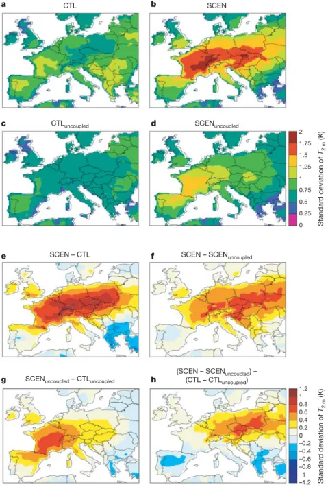
We first analyse how the uncoupling of the land–atmosphere system affects summer temperature variability. Figure 1a–d displays the temperature variability in the four experiments, expressed in terms of the standard deviation of the summer (June–August) two- metre temperature T
2 m(see Methods). Comparison shows that the variability in the SCEN experiment is considerably enhanced, and that the coupling explains a substantial fraction of the simulated future temperature variability (compare Fig. 1b and Fig. 1d). Overall, the effect of soil-moisture–temperature coupling in SCEN amounts to about two-thirds of the climate-change signal (Fig. 1e, f). Figure 1g and h displays a splitting of the total climate-change-induced variability change (Fig. 1e) into respective contributions owing to changes in external factors (atmospheric circulation, sea surface temperatures; Fig. 1g) and changes in land–atmosphere coupling (Fig. 1h; see Supplementary Discussion 2 for details). Disentangling the two signals shows that external effects are mostly restricted to France (Fig. 1g), while variability increases due to land–atmosphere coupling dominate in central and eastern Europe (Fig. 1h). Thus, changes in atmospheric circulation alone are unable to induce the projected increase in temperature variability, and the role of land–
atmosphere coupling needs to be accounted for.
These results led us to ask why we find such a large impact of land–atmosphere coupling for future temperature variability in Europe, when the GLACE study (for present climate) did not
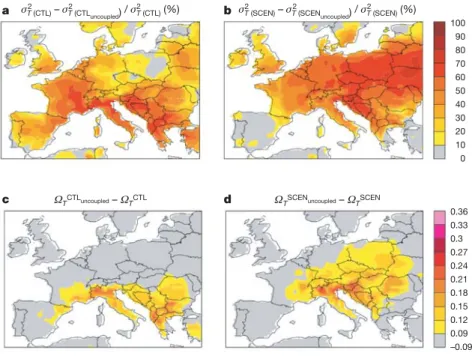
11. Could this be related to climate-change-induced modifications in land–atmosphere coupling characteristics? To address this question, we investigate the land–atmosphere coupling strength in CTL and SCEN using two different measures displayed in Fig. 2 (see Methods).
The results obtained for these two measures are qualitatively similar and present two interesting features: (1) there is a shift of the region of highest soil-moisture–temperature coupling from the Mediterra- nean (CTL) to central and eastern Europe (SCEN); and (2) although
LETTERS
1Institute for Atmospheric and Climate Science, ETH Zurich, Universita¨tsstrasse 16, 8092 Zurich, Switzerland.
Vol 443|14 September 2006|doi:10.1038/nature05095
205
the absolute impact of land–atmosphere coupling on temperature variability is substantially larger in SCEN (Fig. 1b versus Fig. 1a), the fraction of variance explained by land–atmosphere coupling in the Mediterranean, and in central and eastern Europe, respectively, increases only slightly from CTL to SCEN (about two-thirds of the total summer temperature variance in both cases).
We considered possible reasons for the differences in soil-moisture–
temperature coupling in the Mediterranean region compared to the GLACE experiment. Such differences could be due to: (1) the higher resolution of our experiments (56 km compared to 1.88–3.88 or
,100–400 km); (2) representation of interannual variations in seasurface temperatures (SSTs; see Methods); (3) differences in model sensitivity, presumably due to parameter choices
21.
Further analysis based on a large set of RCM and GCM exper- iments from the European project PRUDENCE
22and the Intergo- vernmental Panel on Climate Change (IPCC) Fourth Assessment Report (AR4)’s database, respectively, suggests that our model simulations are consistent with other RCM and GCM experiments (see Supplementary Discussion 1 and Supplementary Figures 1–3). To investigate this further, in Fig. 3 we compare the correlation between
evapotranspiration and temperature (r
ET, T2 m) in our simulations and in the investigated GCMs. This can be seen as a reverse measure of soil- moisture–temperature coupling, as negative correlations point to a strong control of soil moisture upon evapotranspiration and tempera- ture (while positive correlations generally point to a strong atmos- pheric control on evapotranspiration; see Methods). The values of
rET, T2 mfor our RCM experiments show (Fig. 3a, b) an excellent agreement with the measures of soil-moisture–temperature coupling strength (Fig. 2). Figure 3d–i displays
rET, T2 mfor all GCMs (Fig. 3g–i), and for three GCMs (Fig. 3d–f) found to have high-quality circulation patterns in Europe
23. For the CTL time period, the large bands of negative
rET, T2 min the GCMs show patterns clearly similar to those of the ‘hotspots’ of land–atmosphere coupling of the GLACE exper- iment
7,11. However, unlike the GLACE experiment but like our CTL experiment, they include the Mediterranean region (Fig. 2). Thus, it appears that the presence of interannual SST variations is the dominant mechanism explaining the difference between our CTL and the GLACE experiments. (This result is nevertheless qualitatively consistent with the GLACE experiment, because the Mediterranean region is a transi- tional zone between dry and wet climates).
Figure 1|Effects of land–atmosphere coupling on greenhouse-gas induced changes in interannual variability of summer two-metre temperature.
a–d, Standard deviation of summer (June–August) temperature in CTL (a), SCEN (b), CTLuncoupled(c), and SCENuncoupledexperiments (d).e,f, Differences between SCEN and CTL (e) and between SCEN and SCENuncoupled
(f) experiments.g,h, Relative contributions to the climate-change signal of changes in external factors (circulation, sea surface temperatures), computed as SCENuncoupled2CTLuncoupled(g), and changes in land–atmosphere coupling, computed as
ðSCEN2SCENuncoupledÞ2ðCTL2CTLuncoupledÞ(h).
(See text and Supplementary Discussion 2 for more details).
LETTERS
NATURE|Vol 443|14 September 2006206
Concerning the changes in
rET, T2 mbetween present and future climate (Fig. 3c, f, i), a clear shift towards a more soil-moisture- controlled evapotranspiration regime in central Europe can be identified in the simulations. Figure 3 also shows that there are significant differences between GCMs regarding the magnitude of the effect (Fig. 3f, i), and that the RCM experiment (Fig. 3a, b) shows more geographical detail and on average a somewhat lower
atmospheric control on evapotranspiration than the GCM experi- ments (possibly owing to the models’ resolution in the Alpine region).
However, overall the analyses in Figs 2 and 3 are consistent and suggest that our findings are—at least qualitatively—not model specific.
Land–atmosphere coupling affects not only summer temperature variability, but also the whole water cycle in the simulations. Figure 4a–d presents a similar analysis to that of Fig. 1e–h, but for summer
Figure 2|Importance of soil-moisture–temperature coupling in present and future climate in terms of two different coupling diagnostics. a,b, Percentage of interannual summer temperature variance due to land–atmosphere coupling.c,d, Land–atmosphere coupling parameter for temperature computed in analogy to the GLACE experiment. (See Methods for a description of the coupling diagnostics).Figure 3|Correlation of summer (June–August) evapotranspiration and temperature (rET,T2 m) in the RCM and IPCC AR4 GCM experiments.
The three columns display (from left to right) the CTL period (a,d,g), the SCEN period (b,e,h), and the change between the two periods (c,f,i).
The three rows show (from top to bottom): RCM results (a–c); mean of ECHAM5, HADGEM1 and GFDL2.1 GCMs (d–f); mean of all GCMs (g–i).
(See Methods for a description of the analysed GCMs and the computation ofrET,T2 m).
NATURE|Vol 443|14 September 2006
LETTERS
207
precipitation variability. This comparison indicates that in most regions where an increase of precipitation variability is simulated (in particular in the Alpine region), the signal is at least partly caused by land–atmosphere coupling (see Supplementary Discussion 2 for more details). A computation similar to the one presented in Fig. 2b for temperature reveals that land–atmosphere coupling accounts again for about two-thirds of the total summer precipitation variance of the SCEN simulations in regions where increases of sizeable magnitude are simulated. Although there is generally more model uncertainty with regard to changes in precipitation than in tempera- ture variability
3, this result indicates another possibly key effect of land–atmosphere coupling.
In conclusion, the most striking result of our analysis is that land–
atmosphere coupling is significantly affected by global warming and is itself a key player for climate change. Enhanced greenhouse gas concentrations lead to a northwards shift of climatic zones within the European continent. As a consequence, central and eastern Europe becomes a new transitional zone between dry and wet climates (similar to the Mediterranean region in the present climate), and thereby becomes susceptible to the effects of land–atmosphere coupling
7,11. These mechanisms can be identified both in our RCM experiment and in the analysed GCM simulations.
With regards to temperature variability (and associated heat- waves), our study does not contradict earlier reports that emphasized the role of atmospheric circulation changes
5,15,18. Rather, our results show that changes in both circulation and land-surface processes are necessary to explain the projected increase in variability. Here the impact of the circulation changes may be indirect, by imposing changes in the seasonal cycle of soil moisture
24,25, which in turn can lead to modified soil-moisture–temperature coupling characteristics.
Finally, this investigation reveals how profoundly greenhouse gas forcing may affect the functioning of the regional climate system and the role of land-surface processes. At present, measurements of soil moisture
26and evapotranspiration are extremely scarce (particularly in Europe) and do not allow an accurate assessment of these gradual changes. Therefore, a better monitoring of the terrestrial water and energy cycles in mid-latitude regions would be invaluable to further
our understanding of these processes and changes. Ultimately, it could also contribute to improved seasonal forecasting, and thereby help us to cope with the consequences of climate change.
METHODS
RCM climate-change experiments.The climate-change scenario is based on the SRES A2 transient greenhouse gas scenario as specified by the IPCC31. The scenario computations involve three numerical models: the low-resolution HadCM3 global coupled atmosphere–ocean GCM27, the intermediate- resolution HadAM3H atmospheric GCM28, and the CHRM limited-area high- resolution RCM29. For details please refer to previous publications1,3. A summary of the experimental set-up is given in Supplementary Table 1.
GCM climate-change experiments.The simulations are taken from the IPCC AR4 PCMDI data bank (http://www-pcmdi.llnl.gov/ipcc/about_ipcc.php;
20C3M for present-climate and SRES A2 for future-climate experiments). A total of 12 GCM experiments with corresponding variables for the two periods are analysed: ECHAM5*, HADGEM1*, GFDL2.1*, CCCMA_T47, MIR- OC_MED, GISS, HADCM3, INM-CM, IPSL, MRI, NCAR_CCSM, NCAR_PCM. The models with asterisks (*) were recently identified as effectively representing circulation patterns in the northern mid- and high latitudes and in Europe23(the GCMs MIROC_HI and CCCMA_T63 are not available for the SRES A2 scenario period). Some of the analysis in Fig. 3 and the Supplementary Information refers to these three GCMs.
Computation of interannual summer variability of climate variables.The interannual summer variability of temperature and precipitation (Figs 1, 4)—
and other climate variables presented in the Supplementary Information—is defined here as the standard deviation of the June–August mean values. Trend- induced inflation of the standard deviation (and variance, Fig. 2a, b) is removed using linear detrending30. The detrending has some quantitative effect on the results but no significant qualitative impact.
Computation of soil-moisture–temperature coupling parameters.The coup- ling parameters we used are: the variance analysis, the GLACE-type coupling strength parameter, and the correlation between summer temperature and evapotranspiration.
Variance analysis. Figure 2a and b displays (for CTL and SCEN) the percentage of the interannual variance of June–August mean summer temperature that can be explained by land–atmosphere coupling, estimated as:
j2TðcoupledÞ2j2TðuncoupledÞ
j2TðcoupledÞ Figure 4|Effects of land–atmosphere coupling on greenhouse-gas-induced
changes in interannual variability of summer precipitation.
a,b, Differences in standard deviation of summer (June–August) precipitation: SCEN2CTL (a), SCEN2SCENuncoupled(b).c,d, Relative contributions to climate-change signal of changes in external factors
(circulation, sea surface temperatures), computed as
SCENuncoupled2CTLuncoupled(c), and changes in land–atmosphere coupling, computed as (SCEN2SCENuncoupledÞ2ðCTL2CTLuncoupled) (d).
(See text and Supplementary Discussion 2 for more details).
LETTERS
NATURE|Vol 443|14 September 2006208
GLACE-type coupling strength parameter. The soil-moisture–temperature coupling strength parameter for present-day (QCTLT uncoupled2QCTLT ) and future- climate (QSCENT uncoupled2QSCENT ) conditions displayed in Fig. 2c and d is computed in analogy to the approach followed in the GLACE experiment7,11, with adaptations for a 20-year analysis sample. We consider here detrended timeseries of 6-day mean temperature values for June–August (neglecting the first 6-day interval to account for the same period as GLACE, that is, 14 values per summer) for 20 summers (corresponding to the 20 years of simulations considered). First theQCTLT ;QCTLT uncoupled;QSCENT ;andQSCENT uncoupled;values are computed as follows:
QT¼20j2^
T2j2T 19j2T
wherej2Tis the standard deviation of 6-day mean temperature computed from all values available within the respective simulations (that is, 280 values in total) andj2^
Tis the standard deviation of the 6-day mean temperature in the 20-year- average time series (that is, 14 values in total). TheQTvalues are estimates of the degree of interannual similarity in each experiment, so the values (QCTLT uncoupled2QCTLT ) and (QSCENT uncoupled2QSCENT ) represent the extent to which the removal of interannual variability of soil moisture increases the interannual similarity (or decreases the interannual variability) of the simulations. For more details please refer to refs 7 and 11.
We note a few significant differences in the set-up of the present study compared to these earlier analyses7,11. First, our ‘ensemble members’ are simulations for 20 individual summers corresponding to differing SST and atmospheric conditions, whereas the GLACE ensemble members are 16 simu- lations corresponding to one set of SST conditions (1994) but differing atmospheric conditions. Second, our ‘uncoupled’ simulations investigate the impact of prescribing soil moisture to the climatology, that is, two effects are included: (1) it implies the same soil moisture evolution for each year (or each
‘ensemble member’), which induces a zero interannual variation of soil moist- ure; (2) the use of the climatological soil-moisture evolution in each summer induces a damped intra-annual variation of soil moisture. In comparison, the GLACE experiment uses the soil-moisture evolution of one ensemble member in the ‘uncoupled’ simulations, which thus only investigates the impact of zero inter-member differences in soil-moisture evolution but does not damp the intra-annual evolution of soil moisture. The first point is relevant for the possible combination of SST-induced circulation changes with local amplification through land–atmosphere feedbacks; the second point may be more relevant for soil-moisture–precipitation rather than soil-moisture–temperature feed- backs, because increases in precipitation variability are expected to be related to increases in both intra-annual as well as interannual climate variability, while increases in temperature variability (in particular, linked to more frequent heatwaves) are expected to be more typically associated with increases in interannual climate variability.
Correlation between summer temperature and evapotranspiration. Figure 3a, b, d, e, g and h shows for the analysed RCM and GCM experiments the correlation between June–August mean summer temperature and evapotran- spirationrET, T2 mfor the 20 years considered of the CTL and SCEN time periods (computed from detrended timeseries). We note that this measure of coupling is only meaningful in regions where evapotranspiration is not exceedingly small (for example, the Sahara in the GCM simulations or Spain in the RCM SCEN experiment).
Received 12 December 2005; accepted 20 July 2006.
1. Scha¨r, C.et al.The role of increasing temperature variability in European summer heatwaves.Nature427,332–-336 (2004).
2. Giorgi, F., Bi, X. & Pal, J. S. Mean, interannual variability and trends in a regional climate change experiment over Europe. II. Climate change scenarios (1971–- 2100).Clim. Dyn.23,839–-858 (2004).
3. Vidale, P. L., Lu¨thi, D., Wegmann, R. & Scha¨r, C. European climate variability in a heterogeneous multi-model ensemble.Clim. Change(in the press).
4. Ra¨isa¨nen, J. CO2-induced changes in interannual temperature and precipitation variability in 19 CMIP2 experiments.J. Clim.15,2395–-2411 (2002).
5. Meehl, G. A. & Tebaldi, C. More intense, more frequent, and longer lasting heat waves in the 21st century.Science305,994–-997 (2004).
6. Lenderink, G., van Ulden, A., van den Hurk, B. & Van Meijgaard, E. Summertime interannual temperature variability in an ensemble of regional model simulations: analysis of surface energy budget.Clim. Change(in the press).
7. Koster, R. D.et al.Regions of strong coupling between soil moisture and precipitation.Science305,1138–-1140 (2004).
8. Betts, A. K. Understanding hydrometeorology using global models.Bull. Am.
Met. Soc.85,1673–-1688 (2004).
9. Scha¨r, C., Lu¨thi, D., Beyerle, U. & Heise, E. The soil-precipitation feedback: A
process study with a regional climate model.J. Clim.12,722–-741 (1999).
10. Eltahir, E. A. B. A soil moisture-rainfall feedback mechanism. 1. Theory and observations.Water Resour. Res.34,765–-776 (1998).
11. Koster, R. D.et al.GLACE: The Global Land–-Atmosphere Coupling Experiment.
Part 1. Overview.J. Hydrometeor.7,590–-610 (2006).
12. Luterbacher, J., Dietrich, D., Xoplaki, E., Grosjean, M. & Wanner, H. European seasonal and annual temperature variability, trends, and extremes since 1500.
Science303,1499–-1503 (2004).
13. Stott, P. A., Stone, D. A. & Allen, M. R. Human contribution to the European heatwave of 2003.Nature432,610–-614 (2004).
14. Christensen, J. H. & Christensen, O. B. Severe summertime flooding in Europe.
Nature421,805–-806 (2003).
15. Pal, J. S., Giorgi, F. & Bi, X. Consistency of recent European summer precipitation trends and extremes with future regional climate projections.
Geophys. Res. Lett.31,L13202 (2004).
16. Milly, P. C. D., Dunne, K. A. & Vecchia, A. V. Global pattern of trends in streamflow and water availability in a changing climate.Nature438,347–-350 (2005).
17. Frei, C., Scho¨ll, R., Fukutome, S., Schmidli, J. & Vidale, P. L. Future change of precipitation extremes in Europe: An intercomparison of scenarios from regional climate models.J. Geophys. Res.111,D06105 (2006).
18. Ogi, M., Yamazaki, K. & Tachibana, Y. The summer northern annular mode and abnormal summer weather in 2003.Geophys. Res. Lett.32,L04706 (2005).
19. Sutton, R. T. & Hodson, D. L. R. Atlantic ocean forcing of North American and European summer climate.Science309,115–-118 (2005).
20. Koster, R. D., Suarez, M. J. & Heiser, M. Variance and predictability of precipitation at seasonal-to-interannual time scales.J. Hydrometeor.1,26–-46 (2000).
21. Lawrence, D. M. & Slingo, J. M. Weak land–-atmosphere coupling in HadAM3:
role of soil moisture variability.J. Hydrometeor.6,670–-680 (2005).
22. Christensen, J. H., Carter, T. R. & Giorgi, F. PRUDENCE employs new methods to assess European climate change.Eos83,147 (2002).
23. van Ulden, A. O. & van Oldenborgh, G. J. Large-scale atmospheric circulation biases and changes in global climate simulations and their importance for climate change in Central Europe.Atmos. Chem. Phys.6,863–-881 (2006).
24. Findell, K. L. & Delworth, T. L. A modeling study of dynamic and thermodynamic mechanisms for summer drying in response to global warming.Geophys. Res. Lett.32,L16702 (2005).
25. Seneviratne, S. I., Pal, J. S., Eltahir, E. A. B. & Scha¨r, C. Summer dryness in a warmer climate: a process study with a regional climate model.Clim. Dyn.20, 69–-85 (2002).
26. Robock, A.et al.The global soil moisture data bank.Bull. Am. Meteorol. Soc.81, 1281–-1299 (2000).
27. Johns, T. C.et al.Anthropogenic climate change for 1860 to 2100 simulated with the HadCM3 model under updated emissions scenarios.Clim. Dyn.20, 583–-612 (2003).
28. Pope, D. V., Gallani, M., Rowntree, R. & Stratton, A. The impact of new physical parameterizations in the Hadley Centre climate model HadAM3.Clim. Dyn.16, 123–-146 (2000).
29. Vidale, P. L., Lu¨thi, D., Frei, C., Seneviratne, S. I. & Scha¨r, C. Predictability and uncertainty in a regional climate model.J. Geophys. Res.108(D18), 4586, (2003).
30. Scherrer, S. C., Appenzeller, C., Liniger, M. A. & Scha¨r, C. European temperature distribution changes in observations and climate change scenarios.Geophys. Res. Lett.32,L19705 (2005).
31. Nakicenovic, N.et al. IPCC Special Report on Emissions Scenarios(eds Nakicenovic, N. & Swart, R.) (Cambridge Univ. Press, Cambridge, UK, 2000).
Supplementary Informationis linked to the online version of the paper at www.nature.com/nature.
AcknowledgementsThe computations were performed on the computing facilities of ETH Zurich and the Swiss Center for Scientific Computing (CSCS).
We thank the Hadley Centre, UK, for providing access to their climate-change simulations, the PRUDENCE team for earlier interactions and model inter- comparisons (unperturbed simulations), the international modelling groups for providing the IPCC AR4 data through PCMDI, and the GFDL modelling group for access to the GFDL evapotranspiration fields. We acknowledge the JSC/CLIVAR Working Group on Coupled Modelling (WGCM) and their Coupled Model Intercomparison Project (CMIP) and Climate Simulation Panel for organizing the IPCC model data analysis activity, and the IPCC WG1 TSU for technical support.
We also thank our colleagues for comments on the manuscript. This research was supported by the Swiss National Science Foundation (NCCR Climate) and by the sixth Framework Programme of the European Union (project
ENSEMBLES).
Author InformationReprints and permissions information is available at www.nature.com/reprints. The authors declare no competing financial interests.
Correspondence and requests for materials should be addressed to S.I.S.
(sonia.seneviratne@env.ethz.ch).
NATURE|Vol 443|14 September 2006
LETTERS
209