Job Opportunities along the Rural-Urban Gradation and Female Labor Force Participation in India

(1)

Policy Research Working Paper 7412

Job Opportunities along the Rural-Urban

Gradation and Female Labor Force Participation in India

Urmila Chatterjee Rinku Murgai

Martin Rama

Poverty Global Practice Group &

Office of the Chief Economist South Asia Region

September 2015

WPS7412

Public Disclosure Authorized Public Disclosure Authorized Public Disclosure Authorized Public Disclosure Authorized

(2)

Produced by the Research Support Team

Abstract

The Policy Research Working Paper Series disseminates the findings of work in progress to encourage the exchange of ideas about development issues. An objective of the series is to get the findings out quickly, even if the presentations are less than fully polished. The papers carry the names of the authors and should be cited accordingly. The findings, interpretations, and conclusions expressed in this paper are entirely those of the authors. They do not necessarily represent the views of the International Bank for Reconstruction and Development/World Bank and its affiliated organizations, or those of the Executive Directors of the World Bank or the governments they represent.

Policy Research Working Paper 7412

This paper is a product of the Poverty Global Practice Group, and the Office of the Chief Economist, South Asia Region. It is part of a larger effort by the World Bank to provide open access to its research and make a contribution to development policy discussions around the world. Policy Research Working Papers are also posted on the Web at http://econ.worldbank.

org. The authors may be contacted at uchatterjee@worldbank.org The recent decline in India’s rural female labor force par- ticipation is generally attributed to higher rural incomes in a patriarchal society. Together with the growing share of the urban population, where female participation rates are lower, this alleged income effect does not bode well for the empowerment of women as India develops. This paper argues that a traditional supply-side interpretation is insufficient to account for the decline in female participa- tion rates, and the transformation of the demand for labor at local levels needs to be taken into account as well. A salient trait of this period is the collapse in the number of farming jobs without a parallel emergence of other employ- ment opportunities considered suitable for women. The paper develops a novel approach to capture the structure of employment at the village or town level, and allow for

differences along six ranks in the rural-urban gradation. It also considers the possible misclassification of urban areas as rural, as a result of household surveys lagging behind India’s rapid urbanization process. The results show that the place of residence along the rural-urban gradation loses relevance as an explanation of female labor force participa- tion once local job opportunities are taken into account.

Robustness checks confirm that the main findings hold

even when taking into account the possibility of spurious

correlation and endogeneity. They also hold under alter-

native definitions of labor force participation and when

sub-samples of women are considered. Simulations sug-

gest that for India to reverse the decline in female labor

force participation rates it needs to boost job creation.

(3)

Job Opportunities along the Rural-Urban Gradation and Female Labor Force Participation in India

Urmila Chatterjee, Rinku Murgai and Martin Rama The World Bank

^*

JEL Classification: I38, J13, J16, J2, J43, J46, J48, J6, O14, O15

Keywords: Female labor force participation, Jobs, Urbanization, Measurement, India.

*

The corresponding author is Urmila Chatterjee (email: uchatterjee@worldbank.org). The findings,

interpretations, and conclusions expressed in this paper are entirely those of the authors. They do not

necessarily represent the views of the World Bank Group and its affiliated organizations, or those of the

Executive Directors of the World Bank Group or their governments.

(4)

2 1. Introduction

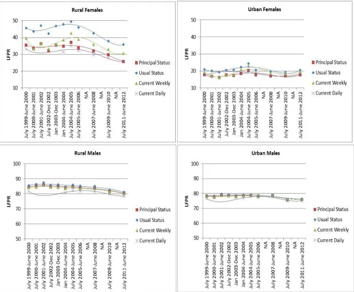
Female labor force participation in India is unusually low. According to the International Labor Organization (2013), India ranks 120 among 131 countries. Even within South Asia, India ranks sixth among eight countries, just above Pakistan and Afghanistan (World Bank, 2012). Two other intriguing patterns stand out when analyzing the labor force participation rate (LFPR) of Indian women aged 15 years and above (figure 1). One is the significant gap between rural and urban areas; the other is the dramatic drop in female LFPR in rural areas after 2004-05.

Figure 1: Female labor force participation is declining in rural areas and has been consistently low in urban areas

Notes and sources: The sources of data are the consumption expenditure surveys and the employment and

unemployment surveys of the National Sample Survey (NSS). Trends are presented for the four definitions of LFPR

used in the NSS. Employment definitions are discussed in the Appendix.

(5)

3 While the LFPR for rural men declined by 3 to 4 percentage points over the period 1999-00 to 2011-12, the magnitude of the decline was much larger for rural women, with their LFPR falling by 8 to 10 percentage points regardless of the measure of employment used. The decline was particularly pronounced after 2004-05, when the female LFPR fell by 12-14 percentage points, in contrast with the much steadier and slower decline in the male LFPR. In urban areas, there was little change in the LFPR of both males and females in this period. But the rural-urban gap in LFPR for females was consistently higher than for males (15-25 percentage points versus 6-10 percentage points).

¹

India’s decline in rural female LFPR has understandably received considerable attention in the public debate. It is intuitively clear that this decline ought to be connected to the large gap in LFPR between rural and urban areas. And the two patterns taken together are a matter for concern. As argued in the recent Gender and Jobs World Development Reports (World Bank, 2011 and 2012) gainful work by women, and especially paid employment, is correlated with their agency at the household level and in society more broadly, contributing to better development outcomes. In a context of rapid urbanization, these two patterns do not bode well for India’s future.

Some decline in LFPR can be expected with development. At a cross-country level, authors such as Goldin (1994) and Paxson et al. (2000) have argued that there is a “U-shaped” pattern in female LFPR. At low levels of income female LFPR tends to be high, as poor people need to work more to maintain a certain standard of living. Moreover, if there is a shift from agriculture to manufacturing, the nature of factory work could discourage women from participating. But as the economy develops and there is an associated expansion in the services sector and fertility rates decline, there could be an increase in LFPR, especially that of educated females. The nature of the jobs in the services sector may be more attractive to females compared to factory work.

In addition, women’s relative wages may rise due to the comparative advantage they have over men in the service sector jobs. Thus, a combination of preferences and relative wages may lead to a higher female LFPR at higher levels of income.

A large body of academic work has also been devoted to explaining the decline of female LFPR in India’s specific case. Its findings are consistent with the country being on the declining portion of the U shape, although with some important nuances. The literature includes studies by Olsen et al. (2006), Chowdhury (2011), Himanshu (2011), Rangarajan et al. (2011), Kannan et al. (2012),

1

Some authors have argued the spike in LFPR in 2004-05 does not square with the general economic trends in

the period preceding the survey (e.g., Sundaram and Tendulkar (2006), Unni and Raveendran (2007) and

Chandrashekhar and Ghosh (2007)). However, the data from the thin year rounds of the NSS shows that LFPR

of females was increasing at a steady rate in the years between 1999-00 and 2004-05 and dropped steadily

thereafter, thus weakening the argument that the NSS 2004-05 survey results are an outlier.

(6)

4 Neff et al. (2012), Abraham (2013), and Klassen and Peters (2013). Most of these studies emphasize supply-side considerations. Some have argued that the lack of crèches and institutional child support for working women contributes to the decline in female LFPR. As the number of multi-generational households shrinks, women with young children would have no choice but to stay at home. Some, including Olsen et al. (2006), Chowdhury (2011), and Neff et al. (2012), have claimed that social and cultural barriers in a predominantly patriarchal society like India can explain women’s work choices. A common interpretation is that higher rural incomes have gradually allowed more rural women to stay at home, a preferred household choice in a predominantly patriarchal society.

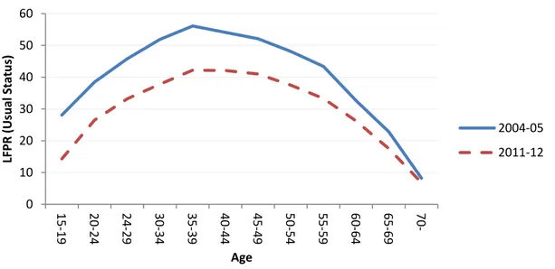
However, supply-side explanations of the decline in female LFPR may not capture the full story in India’s case. Staying longer at school and being less able to rely on family support for child- rearing could justify the LFPR decline for younger women. But they cannot account for the drop in participation among middle-aged cohorts. And the decline in female LFPR between 2004-05 and 2011-12 has been similar across all cohorts aged 15 to 59 (figure 2).

Figure 2: Much of the decline in female labor force participation is for prime working ages

There are also reasons to downplay higher rural wages as the main explanation for the decline in female LFPR. Consider for example the drought of 2009-10, which was amongst the worst in three decades. This negative shock must have resulted in a decline in household earning opportunities in rural areas, in spite of the support provided by transfers programs such as the Mahatma Gandhi Rural Employment Guarantee (MNREGA). Yet, female LFPR did not increase in that year in rural areas, but rather fell dramatically (Himanshu, 2011).

0 10 20 30 40 50 60

15-19 20-24 24-29 30-34 35-39 40-44 45-49 50-54 55-59 60-64 65-69 70-

LF PR (Usu al Status)

Age

2004-05

2011-12

(7)

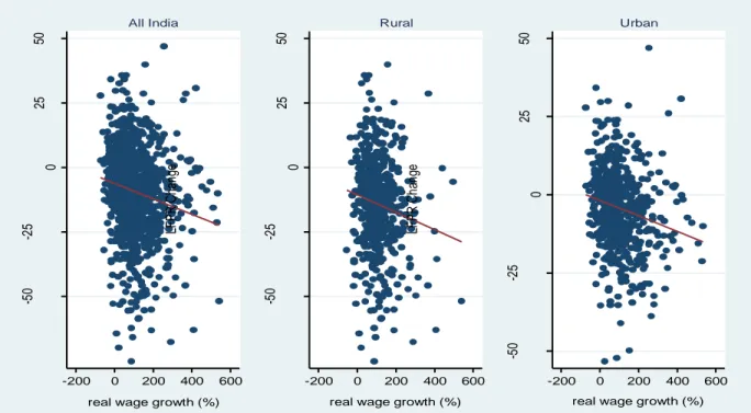
5 A more structured version of this contrarian view involves looking at the relationship between the change in female LFPR and the change in average wages at the district level between 2004- 05 and 2011-12. Based on the income-effect interpretation, one would expect larger declines in female LFPR in districts experiencing a faster increase in average wages. The available evidence confirms that such relationship exists, but its explanatory power is very limited (figure 3). Even taking the estimated relationship at face value, the doubling of average wages in real terms – which is roughly what was observed in practice – would be associated with a reduction in LFPR by about 3 percentage points. The estimate is similar in rural and urban areas (3.4 and 2.5 percentage points respectively). Yet, it is only in rural areas that female LFPR declined substantially, and the observed decline was about three times larger than what this crude district- level relationship would suggest.

Figure 3: Higher wages are associated with only a modest decline in female participation rates at the district level

Notes: District-level changes in average labor force participation rates and real wages during the 2004-05 to 2011-12 period.

This admittedly crude evidence suggests that something else, in addition to supply-side effects, is happening in rural areas. In fact, households with similar living standards are characterized by different female LFPR depending on their place of residence. Monthly per capita expenditures (MCPE) provide a defensible proxy for household income. If all households are classified by

-50-25 02550

LFPR Change

-200 0 200 400 600 real wage growth (%)

All India

-50-25 02550

LFPR Change

-200 0 200 400 600 real wage growth (%)

Rural

-50-25 02550

LFPR Change

-200 0 200 400 600 real wage growth (%)

Urban

(8)

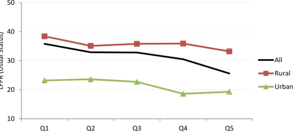
6 quintiles of per capita expenditure, independently of where they live, it is indeed true that female LFPR declines with household income. But to a large extent this is a composition effect, resulting from the higher share of better-off households who reside in urban areas, where female LFPR is lower (figure 4). The relationship between household income and female LFPR is much flatter within both rural and urban areas.

Figure 4: Female participation rates decline with household income at the aggregate level, less so within either rural or urban areas

Notes: Estimates for 2011-12. Quintiles drawn on monthly per capita expenditure, after correcting for cost of living differences between states and rural-urban areas using the official (Tendulkar) poverty lines.

The observed decline in rural female labor force participation may be overstated by the arbitrariness of the administrative rural-urban divide. Much of the growth in India’s urban population in recent years has taken place in administratively rural areas. Thus, what appears to be a decline in rural female LFPR may to some extent be the consequence of urbanization, not a genuinely rural phenomenon.

The Census categorizes urban areas into statutory towns and Census towns. Statutory towns are places with a municipality, corporation, cantonment board or notified town area committee.

Census towns are rural panchayats with urban characteristics. They have a minimum population of 5,000, a density of at least 400 inhabitants per sq. km. and at least 75 percent of their male workers engaged in non-farm work. There has been a multiplication of these Census towns in recent years, with 2,542 of them created between 2001 and 2011, compared to 242 new

10 20 30 40 50

Q1 Q2 Q3 Q4 Q5

LFPR (Usual Statu s)

Quintiles of real monthly per capita consumpt (poorest to richest)

All

Rural

Urban

(9)

7 statutory towns. More than one third of the increase in the urban population over this period came from Census towns.

Even counting Census towns as urban may result in an under-estimation of India’s degree of urbanization. Most countries rely on population size to distinguish between rural and urban areas, usually setting the “tilt-over” threshold in the range of 2,000 to 5,000 inhabitants. Relative to international practice, the criteria used to identify Census towns in India may be too stringent.

If only population size was used to identify urban areas in India, and villages with more than 5,000 inhabitants were considered urban, the share of the rural population would decrease by close to 15 percentage points (Li and Rama, forthcoming).

While the Census may lag behind reality in capturing India’s rapid urbanization, the NSS lags further behind the Census in reclassifying rural areas as urban. The latest round of the NSS on employment and unemployment, conducted in 2011-12, used the Census 2001 as its rural sampling frame. This might have resulted in a considerable underestimation of the share of the urban population, given the unprecedented growth in Census towns between 2001 and 2011.

Part of the apparent decline in rural female LFPR could thus be a composition effect, reflecting urban-type outcomes in officially rural areas.

A few studies have paid attention to demand-side factors to explain the observed decline in female labor force participation. The implicit hypothesis in most cases is that the number and type of jobs available matters. Klassen et al. (2013) focus on female LFPR in urban areas and find that the decline is explained by a combination of rising household incomes and declining white collar jobs, especially for educated women. Rodgers (2012) examines rural Bihar and finds that the decline in female LFPR can be attributed to limited job opportunities for women outside agriculture. Kannan et al. (2012) and Chand et al. (2014) suggest that the decline in female LFPR could be due to poor agricultural performance and the diversification of jobs in rural areas.

The number and type of jobs available also affect the measurement of both work and labor force

participation. According to Hirway (2012), a sizable part of female employment is related to

home-based and subsidiary work, which are not adequately captured by the NSS. Female

unemployment may be underestimated as well. Under the NSS Usual Status and Principal Status

definitions, a person is not considered part of the labor force if he or she has not been looking

for a job for at least six months during the survey year. This is an excessively stringent criterion,

as suggested by two other indicators in the NSS survey. A substantial number of people who

were registered with a placement agency, or who worked or sought worker under MNREGA are

indeed counted by the NSS as being out of the labor force. If their number is taken into account,

female labor force participation would be about 3 percentage points higher in rural areas, and

up to 5 percentage points higher in urban areas (table 1).

(10)

8 Table 1: Female participation rates are much higher when broader measures of unemployment are considered

Notes: Estimates for 2011-12 based on the Usual Status definition of labor force participation.

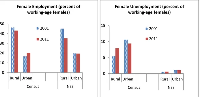
This is consistent with employment indicators from the population Censuses of 2000-01 and 2010-11, which show only a small decline in female participation rates in rural areas compared to the NSS figures for the same time period. The population Census differs from the NSS in what it considers to be employed and unemployed. The broadest measures of employment – “all workers” in the Census and Usual Status in the NSS – yield comparable figures. The main difference between the two sources is in the definition of unemployment. To be counted as unemployed, the Census does not require a person to have been searching for a job for at least six months during the year, as the NSS does. This less stringent definition results in a much higher unemployment rate in rural areas in the Census in 2010-11 (Figure 5). The possible underestimation of unemployment is a hint that jobs became relatively scarcer during this decade, and not all the decline in female labor force participation was voluntary.

This paper takes a fresh look at female labor force participation in India incorporating not only the standard supply-side considerations, but also the demand-side and the urbanization perspectives. This broader view is intuitively articulated in Section 2. Section 3 contains the analytical model underlying the paper. Section 4 presents the empirical strategy and the data used to implement the model. The econometric results are presented in Section 5. Their robustness to problems of spurious correlation, endogeneity and circularity is assessed in Section 6. Section 7 brings together the main findings by decomposing the decline in LFPR between individual effects, household composition effects, urbanization effects, measurement bias and employment effects, along the entire rural-urban gradation. The results suggest that the

LFPR

LFPR adjusted for those recorded as not

in labor force but registered with placement agency

LFPR adjusted for those recorded as not in labor force but who worked/sought work

under MNREGA Males

Rural 81.3 82.9 81.7

Urban 76.4 78.8 76.4

Females

Rural 35.8 38.0 38.4

Urban 20.5 25.3 20.5

(11)

9 changing nature of local job opportunities as India urbanizes accounts for much of the observed decline in female LFPR.

Figure 5: The Census and the NSS tell opposite stories on rural female unemployment

Notes: Estimates from the NSS are from 1999-2000 and 2011-12 survey rounds and based on the Usual Status definition. Estimates from the Census based on the All Workers definition, which combines both main and marginal workers.

2. Location effects

As in other parts of the world, the rapid urbanization process of India has been accompanied by a massive decline in the number of agricultural jobs. What is perhaps more unusual about India is that this structural transformation has not been associated with a substantial increase in manufacturing jobs, or in wage employment. Instead, employment in the services sector has surged. And most of the expansion of employment out of agriculture has been in casual jobs or informal activities.

The central hypothesis of this paper is that the change in job opportunities, and especially the way this change has materialized along the rural-urban gradation, are fundamental to understanding why female LFPR is declining in India. Assessing this hypotheses requires considering labor demand and the rural-urban gradation, in addition to standard individual and household factors, as determinants of female labor force participation.

0 10 20 30 40 50

Rural Urban Rural Urban

Census NSS

Female Employment (percent of working-age females)

2001 2011

0 5 10 15

Rural Urban Rural Urban

Census NSS

Female Unemployment (percent of working-age females)

2001

2011

(12)

10 Casual jobs and informality make the measurement of employment, and hence, the assessment of employment opportunities at the local level, particularly challenging. The NSS defines participation and work in four different ways. In this paper we focus on two definitions that come up often in the discussion on measurement of jobs and their quality, namely Principal Status and Usual Status. Based on Principal Status (PS), a person participates in the labor force is he or she worked or sought work for at least six months over the previous year, and was employed for at least three of those months. Based on Usual Status (US), it is enough to have been employed for at least one month during the previous year to be considered a labor force participant. Thus, the US definition provides a broad measure of participation, whereas the PS definition focuses on a steadier and more regular labor market engagement.

²

Because open unemployment is marginal based on NSS criteria, participation and work are very similar under the PS and US definitions. The difference between employment under the broader US definition and the narrower PS definition is made of subsidiary jobs. These jobs reflect a more tenuous attachment to the labor force.

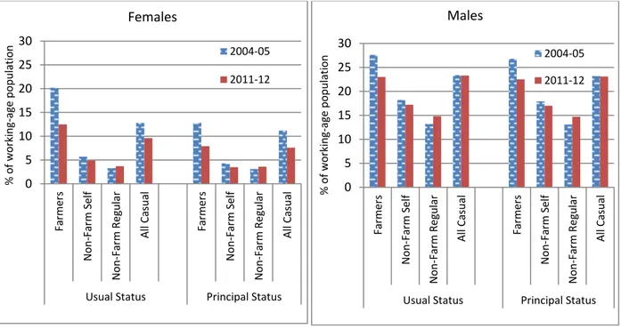
To characterize the employment opportunities available at the local level, in this paper we combine information on activity status and sector of work in the NSS. This allows us to define four types of jobs: farmers, the non-farm self-employed, non-farm regular wage workers, and all casual wage workers. Employment shares can be computed for each of these categories as the ratio of working-age people holding each of the four types of jobs relative to the working-age population. For men, employment shares over the period 2004-05 to 2011-12 are almost identical when using the PS and US definitions (figure 6).

³

For women, on the other hand, the US definition results in higher levels of employment, and therefore, in a higher LFPR. This difference between the US and PS definitions reflects the greater proportion of women engaged in subsidiary work, especially in farming and casual jobs.

Employment shares also reveal a greater diversification of jobs for men than for women, and this is so under both the US and the PS definitions. In rural areas, women’s employment is concentrated in farming and casual jobs. Fewer women work in urban areas, but those who do are typically in non-farm self-employment or in non-farm regular employment (mostly in the services sector).

This lower diversification of employment among women matters, because from 2004-05 to 2011- 12, female farming jobs declined much more rapidly than male farming jobs. Moreover, female farming jobs declined much more under the US definition, implying a sharper decline in

2

The other two definitions include the current weekly status (based on an individual’s activities in the week preceding the survey) and current daily status (which captures the intensity of employment in the week before the survey).

3

With open unemployment being marginal under NSS criteria, working-age people who are out of the labor force

account for the bulk of the left-out group.

(13)

11 subsidiary jobs. There was also a decline in the share of casual jobs for women in rural areas, accompanied by a slight increase in the share of non-farm regular jobs under the PS definition, for both men and women. But the increase took place mainly in urban areas and was not large enough to offset the decline in farming jobs.

Figure 6: The decline in farming jobs in recent years was not offset by an increase in non-farm jobs

The change in the structure of employment at local levels was different along the rural-urban gradation. While most analyses (including the discussion in the introduction to this paper) consider a rural-urban divide, this dichotomous view results in an important loss of granularity.

Urbanization in developing countries has been driven to a large extent by the rapid development of peri-urban areas, beyond formal municipal boundaries, and the densification of officially rural areas. This is even more so in India, where relatively weak city governance has resulted in a particularly “messy” urbanization process.

To better capture the granularity of the rural-urban gradation, this paper introduces a novel approach to classify NSS sampling units along a continuum. Its implementation is described in more detail in section 4. Based on this approach, rural areas fall under one of three ranks based on the average population of a village in the corresponding sampling substratum (below district):

0-999 inhabitants, 1,000-4,999 and 5,000 and above. The selection of these ranks is motivated by the 5000 population size criterion used for the identification of Census towns. Urban areas can be classified into three groups: below 50,000 inhabitants, between 50,000 and one million,

0 5 10 15 20 25 30

Farmers Non-F ar m S el f Non-F ar m Reg ular All Ca su al Farmers Non-F ar m S el f Non-F ar m Reg ular All Ca su al

Usual Status Principal Status

% of wor ki ng -ag e p opulati on

Females

2004-05 2011-12

0 5 10 15 20 25 30

Farmers Non-F ar m S el f Non-F ar m Reg ular All Ca su al Farmers Non-F ar m S el f Non-F ar m Reg ular All Ca su al

Usual Status Principal Status

% of wor ki ng -ag e p opulati on

Males

2004-05

2011-12

(14)

12 and above one million.

⁴

The rural-urban cutoff point considered by the Census is thus located somewhere between the third and the fourth ranks. But taking all six of them into account supports a richer analysis of the impact of location on female LFPR.

There is a striking difference between the LFPR of men and women along this rural-urban gradation. While male LFPR is relatively stable across the six ranks, female LFPR declines quite steadily (figure 7). The definition of employment does not affect the male LFPR but it does result in a different gradient for the decline in female LFPR along the rural-urban gradation. In smaller villages, female LFPR is much higher based on US than it is based on PS. This is because women in rural areas are more frequently engaged in subsidiary work and casual jobs, typically on the farm. The difference in female LFPR between these different definitions of employment shrinks along the rural-urban gradation, and almost completely disappears in large urban centers.

Figure 7: Female labor force participation declines along the rural-urban gradation, as do female subsidiary jobs

Notes: Estimates for 2011-12.

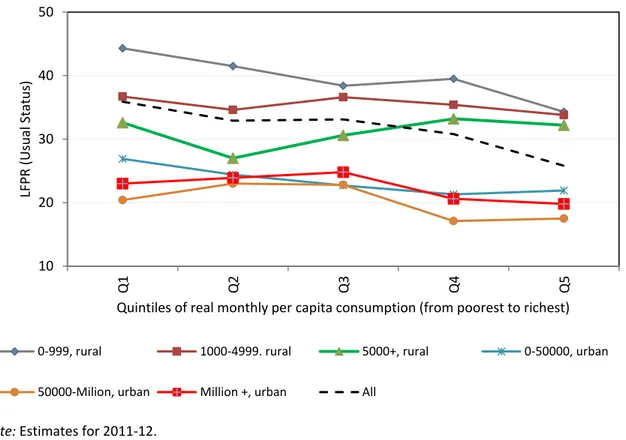
The relationship between monthly per capita expenditures and female LFPR also varies along the rural-urban gradation (figure 8). In both small villages (0-999) and small towns (0-50,000) there is a decline in female LFPR when moving from the bottom consumption quintile to the top. On the other hand, bigger villages and cities experience a more muted decline in female LFPR.

4

Details on the methodology employed to construct the ranks are provided in the next section of the paper.

10 20 30 40 50

0-999, r u ral 1000-4999. rural 5000+, r ur al 0-50000, urban 50000-Mill ion, urban Million + , urban

LFPR

Females

Usual Status Principal Status

50 60 70 80 90

0-999, r u ral 1000-4999. rural 5000+, r ur al 0-50000, urban 50000-Mill ion, urban Million + , urban

LFPR

Males

Usual Status

Principal Status

(15)

13 Figure 8: In large villages and small towns, female labor force participation does not decline with household income

Note: Estimates for 2011-12.

Areas of residence along the rural-urban gradation may differ in many important respects, from infrastructure to amenities. But one key difference between them is the availability of jobs. The structure of employment does not change in a linear way when moving from purely rural to increasingly urban settings. In both 2004-05 and 2011-12 there is a decline in the share of agricultural employment, relative to the working-age population, along the rural-urban gradation (figure 9). But the decline was steady and agricultural jobs were abundant in 2004-05, whereas in 2011-12 there was a sharper drop in agricultural jobs in smaller sized villages. On the other hand, the share of non-farm regular employment is consistently low along the rural-urban gradation, and only picks up modestly in larger urban areas.

In a traditional society, where women’s work is acceptable only if it takes place in environments perceived as safe, female LFPR can be expected to depend on the availability of farming jobs, which are mainly “at home”. From this perspective, in India there is a “valley” of suitable job opportunities along the rural-urban gradation. And in recent years suitable job opportunities for women have declined precipitously in large villages and small towns.

10 20 30 40 50

Q1 Q2 Q3 Q4 Q5

LFPR (Usual Statu s)

Quintiles of real monthly per capita consumption (from poorest to richest)

0-999, rural 1000-4999. rural 5000+, rural 0-50000, urban

50000-Milion, urban Million +, urban All

(16)

14 Figure 9: The availability of jobs considered suitable for women declined sharply in villages and small towns

3. The model

A simple analytical framework can be used to assess the impact of demand-side factors,

characterized by job opportunities and location, on female labor force participation in India. The

(17)

15 framework takes the form of a series of nested specifications for the individual decision to participate in the labor force by working-age women. The standard supply-side specification, called Model A in what follows, emphasizes the characteristics of the woman making the decision and those of her household. It also allows for changes over time in household preferences regarding participation:

𝑃

_𝑖𝑗^∗

= 𝑓

_𝐴

(𝑋

_𝑖𝑗

, 𝐻

_𝑖𝑗

, 𝑡, 𝜀

_𝑖𝑗

)

where:

𝑃

_𝑖𝑗^∗

is the binary choice of participating in the labor force by woman 𝑖 in location 𝑗.

𝑋

_𝑖𝑗

are the characteristics of the woman making the decision, including her age, education, marital status, and number of children.

𝐻

_𝑖𝑗

are the characteristics of her household, including its composition by age and gender, its asset ownership, its social group, and its religion.

𝑡 is the year.

𝜀

_𝑖𝑗

is an independently distributed stochastic disturbance with zero mean.

This basic specification can be enriched so as to take into account the characteristics of the area where the household lives, which yields Model B:

𝑃

_𝑖𝑗^∗

= 𝑓

_𝐵

(𝑋

_𝑖𝑗

, 𝐻

_𝑖𝑗

, 𝑡, 𝑅

_𝑗

, 𝜀

_𝑖𝑗

)

where:

𝑅

_𝑗

is the rank of the area the household lives in along the rural-urban gradation.

The paper argues that in a context of rapid urbanization, the misclassification of actually urban areas as rural can result in estimation biases. This hypothesis is captured in Model C:

𝑃

_𝑖𝑗^∗

= 𝑓

_𝐶

(𝑋

_𝑖𝑗

, 𝐻

_𝑖𝑗

, 𝑡, 𝑅

_𝑗

, 𝐺

_𝑗

, 𝜀

_𝑖𝑗

)

(18)

16 where:

𝐺

_𝑗

is the potential misclassification of the area where the woman lives as rural.

A central hypothesis of this paper is that location matters not just in itself, but because the job opportunities available for women along the rural-urban gradation are different. This gives us the broadest specification, called Model D:

𝑃

_𝑖𝑗^∗

= 𝑓

_𝐷

(𝑋

_𝑖𝑗

, 𝐻

_𝑖𝑗

, 𝑡, 𝑅

_𝑗

, 𝐺

_𝑗

, 𝑂

_𝑖𝑗

, 𝜀

_𝑖𝑗

)

where:

𝑂

_𝑖𝑗

are the local employment opportunities faced by the woman making the decision, both in terms of the number of jobs available and their type.

The key hypotheses to be tested are:

1. When there are better job opportunities in the area where the household lives, other things equal the probability for a women to participate in the labor force is higher.

𝜕𝑓

_𝐷

(. )

𝜕𝑂

_𝑖𝑗

> 0

2. The misclassification of urban areas as rural biases the estimates. It makes the effect of urbanization on participation look as a change in participation within rural areas.

𝜕𝑓

_𝐷

(. )

𝜕𝐺

_𝑗

< 0

3. Not taking into consideration the location where people live, including the possible misclassification of urban areas as rural, and their employment structure, biases the estimates of individual and household effects.

𝜕𝑓

_𝐴

(. )

𝜕𝑋

_𝑖𝑗

≠ 𝜕𝑓

_𝐷

(. )

𝜕𝑋

_𝑖𝑗

𝜕𝑓

_𝐴

(. )

𝜕𝐻

_𝑖𝑗

≠ 𝜕𝑓

_𝐷

(. )

𝜕𝐻

_𝑖𝑗

4. When the employment structure is not taken into

account, the role of urbanization in accounting for the declining LFPR is over-estimated.

| 𝜕𝑓

_𝐵

(. )

𝜕𝑅

_𝑗

| > | 𝜕𝑓

_𝐷

(. )

𝜕𝑅

_𝑗

|

(19)

17 5. The standard supply-side specification attributes to a change in preferences a decline in LFPR actually due to a change in employment opportunities.

𝜕𝑓

_𝐴

(. )

𝜕𝑡 < 𝜕𝑓

_𝐷

(. )

𝜕𝑡

4. Empirical strategy and data

The main difficulty in implementing this model empirically is that the job opportunities faced by women at the local level are not directly observable. In labor economic analyses for industrial countries, job opportunities are assessed through the wage the women could earn. But this wage is not directly observable either. Indeed, women who do not work do not earn any wage. And for those who do work, their own wage is influenced by their personal characteristics and not only by job opportunities. A strategy that has become standard to address these issues is to simultaneously estimate a labor force participation function and a wage function, and to use the estimated parameters to predict the potential wage of working-age women on the basis of their observable characteristics, including their educational attainment, their work experience and their number of young children (Heckman 1974 and 1993).

This strategy is arguably less reliable when applied to developing countries, due to different nature of their employment structures. A majority of workers in industrial countries are wage earners, but most workers in developing countries are farmers or self-employed (World Bank, 2012). The prediction of potential wage earnings in developing countries is thus based on a much smaller sample, relative to the size of the labor force. And this smaller sample is potentially biased by self-selection, as wage earners are unlikely to be a random subset of the people at work. An additional bias often comes from the fact that surveys such as the NSS do not capture comparable wage information for all wage earners.

Other studies introduce labor market indicators as determinants of labor force participation. Job

opportunities have been shown to have two opposite effects on participation. These effects can

be illustrated by considering an unanticipated decline in labor demand. As the prospect of finding

a job becomes more elusive, there is a “discouraged worker” effect: people simply abandon their

job search and withdraw from the labor force. At the same time, as breadwinners lose their jobs,

more spouses – typically housewives – seek employment to compensate for the decline in

household income; this leads to an “added worker” effect. The magnitude of the former effect

has generally been assessed using time series data, which allows to estimate the elasticity of the

aggregate participation rate to the aggregate unemployment rate (Blundell et al. 1988, Blundell

et al. 1993). The second effect has been quantified by looking at spouses’ transitions in and out

of the labor force as their husbands transition in and out of employment (Lundberg 1985 and

Maloney 1987, among others).

(20)

18 Implementing this alternative strategy in developing countries is problematic as well. Measuring unemployment is difficult in a context where most people work for themselves. The sizeable gap between labor force participation rates depending on whether those registered with placement agencies or participating in the MNREGA program are counted in illustrates that difficulty. The different trends in unemployment rates depending on whether the Census or the NSS definitions are used show that even determining whether job opportunities are becoming scarcer or not can be challenging in practice.

This paper adopts a different strategy. The job opportunities faced by women are shaped by the situation of the local labor market. In the basic specification, tested for robustness further down, the job opportunities faced by the woman making the decision take the following form:

𝑂

_𝑖𝑗

= 𝐿

_𝑗

+ 𝑉

_𝑗

− 𝑈

_𝑗

+ 𝜑

_𝑖𝑗

where:

𝐿

_𝑗

is the local employment level, which can be disaggregated into farming, non-farm self-employment, non-farm regular wage employment and casual employment.

𝑉

_𝑗

are local vacancies.

𝑈

_𝑗

is local unemployment.

𝜑

_𝑖𝑗

is the subjective assessment of local job opportunities by the woman making the decision to participate; this assessment is supposed to be independently distributed and to have zero mean.

Replacing in the individual decision to participate yields:

𝑃

_𝑖𝑗^∗

= 𝑓

_𝐷

[𝑋

_𝑖𝑗

, 𝐻

_𝑖𝑗

, 𝑡, 𝑅

_𝑗

, 𝐺

_𝑗

, 𝐿

_𝑗

, (𝑉

_𝑗

− 𝑈

_𝑗

), (𝜀

_𝑖𝑗

+ 𝜑

_𝑖𝑗

)]

In words, labor force participation depends on the individual characteristics of the woman

making the decision (𝑋

_𝑖𝑗

), the characteristics of her household (𝐻

_𝑖𝑗

), the year (𝑡), the rank in the

rural-urban gradation of the location she lives in (𝑅

_𝑗

), the potential misclassification of that

location as urban (𝐺

_𝑗

), and job opportunities at the local level. The latter are captured in two

ways: local employment (𝐿

_𝑗

) and local excess demand for labor (𝑉

_𝑗

− 𝑈

_𝑗

). The former can be

measured using NSS data. The latter is unobservable but can be included in the estimation as a

(21)

19 fixed location-specific effect. As for the last term (𝜀

_𝑖𝑗

+ 𝜑

_𝑖𝑗

), it is an error independently distributed across households and has zero mean, so it does not affect the estimation.

Models A, B, C and D are estimated as Probit regressions using data from the 61

^st

(2004-05) and 68

^th

(2011-12) rounds of the NSS employment and unemployment surveys. Observations are at the individual level, but some variables (those indexed by “j” as opposed to “ij”) need to be constructed at a more aggregate level.

The potential misclassification of urban areas as rural (𝐺

_𝑗

) is measured at the district level, as the difference between the true share of the urban population in the district the household lives in and the urban share estimated based on the NSS. The true urban share is computed on the basis of Census data for 2001 and 2011, treating all villages with more than 5,000 inhabitants as urban, to take into account the fact that the Census uses a rather restrictive definition of urban areas compared to standard international practice.

To capture the diversity of job opportunities in the local labor market, the employment variable (𝐿

_𝑗

) is computed at the substratum level (below district). An innovation of this paper is the approach used to construct indicators below the district level and at the level of the village or town, along six ranks in the rural-urban gradation.

Both the 61

^st

and the 68

^th

rounds of the NSS use the Census 2001 as the sampling frame for rural areas.

⁵

The rural sample is representative at the sampling substratum (below district) level.

Linking the Census to the NSS at the substratum level allows us to reclassify rural areas in every district based on the average village size of the substratum. By doing so, we can construct employment variables for each substratum for rural areas and thereby control for the local labor market structure. We reclassify rural areas into three ranks based on the average population size of a village in a substratum: 0-999, 1,000-4,999 and 5,000 and above. We are able to match 571 districts in the NSS 61

^st

round and 595 districts in the NSS 68

^th

round with the Census 2001 districts.

⁶

This procedure cannot be replicated for the other three ranks considered in this paper, as the NSS uses the Urban Frame Survey (UFS) for urban areas, instead of the Census. Moreover, in urban areas the NSS data is not representative below the district level. For the urban sample we therefore use the population size of the location (below 50,000, between 50,000 and one million, and above one million) to attribute the rank, but construct the employment variables at the district level.

The description of the variables used in the regressions and their descriptive statistics are in Tables 2 and 3 respectively. As noted there, local employment (𝐿

_𝑗

) is disaggregated by type of

5

The exception is Kerala, where the panchayat wards are used as the sampling frame.

6

For the districts that were created after 2001, we merge the data of the new district with its parent to ensure

comparability over time. Also, due to missing substrata information we drop two states (Delhi and Nagaland)

and two Union Territories (Daman and Diu and Andaman and Nicobar Islands).

(22)

20 job, including farming, non-farm self-employment, casual work and non-farm regular wage employment, to reflect the potentially different suitability of alternative job opportunities from women’s point of view.

Table 2: Description of variables used in the empirical analysis

Variables Definition

Dependent Variable

Independent Variables Individual Variables

Age Age (Years)

age_sq Age Squared (Years)

schooling Number of years of schooling (Lahiri et. al. 2013)

schooling_sq Schooling Years Squared

marital_dummy Whether currently married or not

Household Variables

log_landown Log of Land Owned by Household (in hectares)

log_hhsize Log of Household Size

children_under_6 Share of Children below 6 years in the household

children_above_6 Share of Children 6 years or more in the household

female_adult Share of female adults in the household aged 15-59

female_dependent Share of female dependents (aged 60+) in the household

male_dependent Share of male dependents (aged 60+) in the household

female_hh_dummy Household head is a female or not

max_schooling Maximum schooling of household

st_dummy Household belong to Scheduled Tribes or not

sc_dummy Household belong to Scheduled Castes or not

obc_dummy Household belong to Other Backward Castes or not

hindu_dummy Household belongs to Hindu religion

muslim_dummy Household belongs to Muslim regilion

Time Variable

survey NSS61 =1, NSS68=2

Indicator Variable for Location

Average size of village in substratum for rural, Type of stratum for urban rank

Population (0-999=1, 1000-4999=2, 5000-9999=3, 10000>=4) for rural Below million=5, Million plus=6 for urban

Misclassification of urban areas

gap Urban share in Census (based on 5000 population)-Urban share in NSS, district level

Employment Variables (Substratum /district level for rural , district level

for urban) all=Usual Status, Working Age Population =Population 15 years and above

all_farmers_share Share of Agricultural Self Empoyed and Regular workers aged 15+ in working age population all_non_farm_self_share Share of Non Farm Self Empoyed workers aged 15+ in working age population

all_casual_share Share of All Casual workers aged 15+ in working age population

all_non_farm_regular_share Share of Non Farm Regular Wage workers aged 15+ in working age population

Labor Force Participation (Usual Status) for persons aged 15 years and above

(23)

21 Table 3: Mean values of variables used in the empirical analysis

NSS 61 NSS 68

labor force participation 0.46 0.32

age 36.60 37.38

age_sq 1593.10 1654.60

schooling 3.46 4.54

schooling_sq 31.56 43.70

marital_dummy 0.72 0.72

log_land -2.28 -2.58

log_land_sq 11.66 12.73

log_hhsize 1.64 1.57

share children_under_6 0.07 0.06

share children_above_6 0.09 0.09

share female_adult 0.20 0.22

share female_dependent 0.05 0.06

share male_dependent 0.04 0.05

female_headed_household 0.11 0.12

max_schooling_household 7.69 8.84

st_dummy 0.08 0.09

sc_dummy 0.19 0.19

obc_dummy 0.41 0.44

hindu_dummy 0.83 0.82

muslim_dummy 0.12 0.13

survey 1.00 2.00

_Irank_2 0.43 0.41

_Irank_3 0.17 0.15

_Irank_4 0.06 0.07

_Irank_5 0.11 0.11

_Irank_6 0.05 0.06

gap 0.18 0.20

all_farmers_share 0.26 0.19

all_non_farm_self_share 0.12 0.11

all_casual_share 0.19 0.17

all_non_farm_regular_share 0.07 0.08

5. Main results

The four models presented above are estimated for all women aged 15 years and above, with

participation defined based on the US definition of employment in the NSS (table 4). The

estimated marginal effects are reported for each explanatory variable in all four models. Marginal

effects indicate by how much the probability of labor force participation changes for a unit

increase in the corresponding explanatory variable.

(24)

22 Table 4: Marginal probability effects for working-age women based on usual status

Dependent Variable: Labor Force Participation

Model A Model B Model C Model D Model D1

Age 0.045* 0.046* 0.046* 0.052* 0.052***

age_sq -0.001* -0.001* -0.001* -0.001* -0.001***

schooling -0.034* -0.033* -0.033* -0.038* -0.031***

schooling_sq 0.002* 0.002* 0.002* 0.003* 0.002***

marital_dummy -0.055* -0.058* -0.058* -0.060* -0.064***

log_land 0.040* 0.034* 0.033* 0.007* 0.003*

log_land_sq 0.003* 0.004* 0.004* -0.001 -0.001***

log_hhsize -0.056* -0.052* -0.053*** -0.011 -0.005

children_under_6 -0.066* -0.080* -0.080* -0.085* -0.099***

children_above_6 0.069* 0.060* 0.060* 0.117* 0.099***

female_adult 0.033 0.031 0.033 0.040 0.079***

female_dependent 0.057* 0.056* 0.056* 0.046 0.098***

male_dependent 0.135* 0.140* 0.141* 0.140* 0.185***

female_hh_dummy 0.133* 0.133* 0.134* 0.141* 0.160***

max_schooling -0.012* -0.009* -0.010* -0.012* -0.008***

st_dummy 0.220* 0.202* 0.200* 0.135* 0.101***

sc_dummy 0.093* 0.077* 0.077* 0.077* 0.072***

obc_dummy 0.072* 0.065* 0.066* 0.050* 0.047***

hindu_dummy -0.057* -0.056* -0.056* -0.023* -0.049***

muslim_dummy -0.173* -0.165* -0.164* -0.095* -0.118***

survey -0.110* -0.116* -0.115*** -0.003 0.005

rank==2 -0.022* -0.020* 0.012** 0.008*

rank==3 -0.044* -0.032* 0.024* 0.030*

rank==4 -0.117* -0.114* 0.084* 0.082*

rank==5 -0.167* -0.165* 0.030* 0.022

rank==6 -0.154* -0.157* 0.033* 0.018

gap -0.052* -0.051 0.086*

all_farmers_share 1.617* 1.834*

all_non_farm_self_share 1.645* 1.865*

all_casual_share 1.525* 2.066*

all_non_farm_regular_share 1.559* 1.765*

District Fixed Effects No No No Yes No

Number of Observations 317046 317046 317046 316978 317046

Wald Chi Sq 13869 15716 15831 33169 26706

Pseudo R2 0.13 0.14 0.14 0.28 0.26

note: * p<0.01, p<0.05, * p<0.1

In the estimation, the fixed location-specific effects intended to capture the tightness of the labor

market (𝑉

_𝑗

− 𝑈

_𝑗

) are defined at the district level. This choice is guided by computational

limitations and will be revised in subsequent versions of the paper. Introducing a large number

of fixed effects in a Probit regression can bias the estimates. To account for this risk, model D was

(25)

23 also estimated without fixed effects (table 4, fifth column, Model D1). The coefficients and marginal effects being quite similar to those obtained with fixed effects, and the explanatory power of the regression was not much lower. In light of this, the full estimation for Model D, including fixed effects, is retained in what follows as the preferred specification.

The estimated marginal effects under Model A are broadly consistent with the conventional wisdom. The income effect cannot be inferred directly, as monthly expenditures per capita are endogenous and therefore cannot be used as an explanatory variable. But educational attainment is predetermined and provides a good proxy for income generation potential. The marginal effects for the education variable do reflect an inverted-U pattern, with participation first decreasing with schooling, and then increasing. The turning point where higher educational attainment leads to higher LFPR is at the secondary level.

The marginal effect of land ownership is positive, indicating that women tend to participate more when the household owns land. This effect would be consistent with the notion that women are more willing to take jobs that are considered suitable for them, such as working on the family farm. On the other hand, if land ownership is seen as a proxy for income generation potential, this result would contradict the hypothesis of a negative income effect on LFPR.

The estimates for Model A confirm the conventional wisdom regarding the role of marriage and child-rearing in depressing the female LFPR. Married women and women in households with higher share of young children (ages six and below) are less likely to participate in the labor force.

Having older parents or other elderly members in the household does increase LFPR, consistent with the hypothesis that lack of child support constraints women’s ability to participate.

Consistent with the first hypothesis, the marginal effects of the employment shares are positive and highly significant in Model D, implying that the availability of jobs at the local level increases LFPR. The hypothesis that the coefficients of all the employment variables are the same can be rejected at 1 percent significance level. Pairwise Wald tests are however unable to reject the hypothesis that the coefficients on the different types of jobs are statistically different from each other, with the exception of farm employment and casual wage employment. This supports the notion that women view some jobs more suitable than others and that casual wage jobs are viewed differently from farming, non-farm self-employment and non-farm regular wage jobs.

While most individual and household effects remain statistically significant across specifications, their magnitudes are attenuated when going from Model A to Model D, in line with the third hypothesis.

In particular, the returns to schooling are higher for secondary and higher levels of education

when local employment opportunities are controlled for (figure 10). The U-shaped curve for

education becomes steeper for levels secondary and above, implying higher labor force

participation for a given level of education. Most of the expansion in educational attainment of

(26)

24 females between 2004-05 and 2011-12 was in the secondary and above levels. The share of females in the working age population with secondary or above education increased by more than 10 percentage points during this period. A steeper, upward sloping curve implies that the income effect is weaker than what the conventional wisdom would imply.

Figure 10: Controlling for local employment attenuates the impact of asset ownership, implying a weaker income effect

Land ownership becomes less relevant too. The corresponding marginal effect is close to zero when the local employment structure is taken into account. One interpretation of this change is that land ownership was capturing the availability of jobs considered suitable for women. The share of farming jobs at the local level may be a more precise indicator of such availability, thus reducing the explanatory power of the land ownership variable. But land ownership can also be seen as an indicator of income generation potential. If so, the absence of an effect on LFPR can be seen as rejecting the income effect hypothesis.

Similarly, the effect of household size changes substantially. In Models A, B and C, female labor force participation was lower among bigger households, but the household size has no bearing on labor force participation of females in Model D. When employment and urbanization are factored in the participation decisions, the effects of the individual’s social group or religion are attenuated. On the other hand, the effects of having children are enhanced.

The second hypothesis, which is that the misclassification of urban areas as rural matters, is supported in the model without the location fixed effects, but is rejected when district fixed

0.2 0.3 0.4 0.5 0.6

0 2 5 8 10 12 15 17

Pr ob abili ty LFPR

Schooling Years Model A Model B Model C Model D

0.1 0.2 0.3 0.4 0.5 0.6

-0.5 -0.1 0.3 0.7 1.1 1.5 1.9

Pr ob abili ty LFPR

Log Land Owned

Model A

Model B

Model C

Model D

(27)

25 effects are included in the estimation of Model D. This can be seen by comparing the coefficients of the gap variable in the fourth and the fifth columns of table 4.

The fourth hypothesis in this paper is that the impact of urbanization on the LFPR is overstated in the standard analyses. This hypothesis is confirmed by the estimation results too. Specifications not controlling for local employment opportunities and for the possible misclassification of urban areas as rural suggest that urbanization leads to a reduction in the female LFPR. But based on Model D, it is not urbanization by itself that causes the decline. For a similar local employment structure, the actual rank in the rural-urban gradation becomes mainly irrelevant. There is virtually no difference in the participation rates between smaller sized villages and larger sized towns (figure 11). Thus, the jobs around where a household lives, and not where it lives per se, matter for female LFPR.

Figure 11: Urbanization by itself does not lead to lower female labor force participation

Finally, the claim that household preferences in India are becoming more aligned with a patriarchal culture becomes much weaker when relying on the broader specification. Consistent with the fifth hypothesis in this paper, the marginal effect of the time variable decreases by two orders of magnitude and becomes insignificant when moving from Model A to Model D.

0.2 0.3 0.4 0.5 0.6

0-999 , r ural 1000 -4999 . ru ra l 5000 +, rural 0-500 00, urba n 5000 0-M illi on, u rban Mil lio n +, u rb an

Pr obab ility LFPR

Model B

Model C

Model D

(28)

26 6. Robustness checks

The empirical strategy employed in the paper to incorporate demand factors could be challenged on statistical grounds. When job opportunities are assessed through the potential wage of the woman making the decision to participate, as in one of the strategies traditionally used to study female labor force participation in industrial countries, quite a lot of effort goes into addressing the potential wage endogeneity. Wages are observed only for women who work – hence participate in the labor force – and are also affected by individual characteristics bearing no correlation with the availability of job opportunities. Corrections of that sort are not introduced in the other traditional strategy to study female labor force participation in industrial countries, which treats unemployment rates or job losses by husbands as exogenous indicators of job opportunities – or lack thereof. The question is whether the strategy this paper to estimate model D, hence to derive its main conclusions, could be subject to biases requiring correction.

Introducing local employment levels (𝐿

_𝑗

) as a determinant of labor force participation by women raises two potential problems. The first one, spurious correlation, arises when the number of individual observations from the NSS available for some localities is limited. In those localities, a working woman captured by the NSS sample is by definition a labor force participant (𝑃

_𝑖𝑗^∗

= 1) but she also boosts the observed local employment level (𝐿

_𝑗

). The employment shares in Model D are calculated at the substratum level for the rural sample. Although the NSS data is representative for the rural sample at that level, sample sizes are in some cases small. As a result, the number of women working in a particular type of job at the substratum level could be small too, in which case the marginal effect of local employment on labor force participation would be overestimated.

The standard approach to deal with this problem is to use instrumental variables. Fortunately, the Census collects information on the economic activities of individuals in a manner that is similar to that of the NSS, but is totally independent from it. More specifically, the Census allows to compute district-level shares of cultivators, agricultural laborers, household industry workers and others, relative to the population aged 6 years and above. These shares can be computed for both the rural and urban areas of each district using data from the 2001 and 2011 Censuses.

These Census district shares involve very large numbers of people, so are unlikely to be affected by sample size issues. Therefore, Census employment shares at the district level arguably provide a valid instrument for the substratum employment shares in the NSS.

To implement this approach, in the first stage we perform Ordinary Least Squares (OLS)

regressions for the NSS substratum level employment shares, based on usual status. The

corresponding district-level employment shares from the Census, the rank variable and the

interactions between the two, serve as the explanatory variables in these first-stage OLS

(29)

27 regressions. Employment shares from the 2001 Census are used for estimating NSS 2004-05 employment shares, and employment shares from the 2011 Census for the NSS 2011-12 employment shares. The regressions are run separately for the rural and urban samples. The predicted employment shares from the first-stage regressions are then used in the second-stage Probit estimation of female labor force participation.

⁷

When applying this instrumental variables approach to Model D, the five hypotheses advanced in this paper hold (table 5, third column, Model D2). With minor nuances, the marginal effects are similar in size to the marginal effects in the original specification. Only a few differences with the main results in the previous section stand out. Among the household variables, on the one hand, the effect of having dependents in the family is diluted, but on the other, the effect of household size is negative and significant. Some of the location variables, captured by the rank variable, are no longer statistically significant. The survey variable is now slightly significant, but still three times smaller in magnitude than in Model C, where the local employment structure has not been controlled for. The gap variable is now statistically significant. While the effects of the employment variables are attenuated, they are still quite strong and highly significant. In particular, farming jobs have a higher marginal effect than other types of jobs. Regardless of whether there is a job deficit at the aggregate level in India, the gradual disappearance of farming jobs remains a highly significant determinant of the decline in female labor force participation.

⁸

The second potential problem with the empirical strategy of this paper, endogeneity, arises if local employment levels (𝐿

_𝑗

) are correlated with the error term 𝜀

_𝑖𝑗

+ 𝜑

_𝑖𝑗

. Consider a dynamic locality, where many firms operate and more of them are about to start operations. The participation variable (𝑃

_𝑖𝑗^∗

) and the employment variable (𝐿

_𝑗

) will be inflated by the unusually high number of women already at work in the locality. But the participation variable will be inflated even further by the unusually high number joining the labor force to seize the upcoming job opportunities. An analysis not controlling for the firms that are about to start operations will overestimate the effect of current employment on labor force participation. The problem would be symmetric if local unemployment was high.

The introduction of the indicator of labor market tightness at the local levels, (𝑉

_𝑗

− 𝑈

_𝑗

), is supposed to address the two symmetric problems in this example. But it can be argued that it does not address endogeneity if the correlation between local employment levels (𝐿

_𝑗

) and the error term (𝜀

_𝑖𝑗

+ 𝜑

_𝑖𝑗

) occurs across the entire sample, and not only in particularly buoyant or declining localities.

7

The estimated coefficients in the first-stage regressions are significant at the conventional levels; the F-statistics are above 10 in all cases.

8

The hypothesis that the coefficients of all the employment variables are the same can be rejected at 1 percent

significance level.

(30)