Universit¨ at Regensburg Mathematik
Noether-like theorems for causal variational principles
Felix Finster and Johannes Kleiner
Preprint Nr. 11/2015
arXiv:1506.09076v1 [math-ph] 30 Jun 2015
CAUSAL VARIATIONAL PRINCIPLES
FELIX FINSTER AND JOHANNES KLEINER JUNE 2015
Abstract. The connection between symmetries and conservation laws as made by Noether’s theorem is extended to the context of causal variational principles and causal fermion systems. Different notions of continuous symmetries are introduced.
It is proven that these symmetries give rise to corresponding conserved quantities, expressed in terms of so-called surface layer integrals. In a suitable limiting case, the Noether-like theorems for causal fermion systems reproduce charge conservation and the conservation of energy and momentum in Minkowski space. Thus the con- servation of charge and energy-momentum are found to be special cases of general conservation laws which are intrinsic to causal fermion systems.
Contents
1. Introduction and Statement of Results 2
2. Preliminaries 3
2.1. The Classical Noether Theorem 3
2.2. Causal Variational Principles in the Compact Setting 4
2.3. The Concept of Surface Layer Integrals 6
3. Noether-Like Theorems in the Compact Setting 7
3.1. Symmetries of the Lagrangian 7
3.2. Symmetries of the Universal Measure 9
3.3. Generalized Integrated Symmetries 10
4. The Setting of Causal Fermion Systems 11
4.1. Basic Definitions and the Euler-Lagrange Equations 11
4.2. Noether-Like Theorems 14
5. Example: Current Conservation 17
5.1. A General Conservation Law 17
5.2. Correspondence to Dirac Current Conservation 18
5.3. Clarifying Remarks 28
6. Example: Conservation of Energy-Momentum 30
6.1. Generalized Killing Symmetries and Conservation Laws 30 6.2. Correspondence to the Dirac Energy-Momentum Tensor 32
7. Example: Symmetries of the Universal Measure 36
8. Outlook: Conservation Laws in Quantum Space-Times 37
References 38
1
1. Introduction and Statement of Results
In modern physics, the connection between symmetries and conservation laws is of central importance. For continuous symmetries, this connection is made mathemati- cally precise by Noether’s theorem [26]. In recent years, the theory of causal fermion systems was proposed as an approach to describe fundamental physics. Giving quan- tum mechanics, general relativity and quantum field theory as limiting cases, it is a candidate for a unified physical theory (see the review [16] and the references therein).
In the present article, we explore symmetries and the resulting conservation laws in the framework of causal fermion systems. We prove that there are indeed conservation laws, which however have a structure which is quite different from that of the classical Noether theorem. These conservation laws are so general that they apply to “quantum space-times” which cannot be approximated by a Lorentzian manifold. We prove that in the proper limiting case, our conservation laws simplify to charge conservation and the conservation of energy and momentum in Minkowski space. Thus the conservation laws of charge and energy-momentum can be viewed as special cases of more general conservation laws which are intrinsic to causal fermion systems.
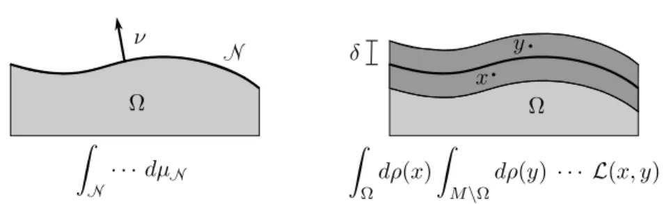
In order to make the paper easily accessible and self-contained, we develop our concepts step by step. Section 2 provides the necessary background: After a brief review of the classical Noether theorem (Section 2.1), we introduce causal variational principles in the compact setting (a mathematical simplification of the setting of causal fermion systems; see Section 2.2). This makes it possible to describe the mathematical structure of our conservation laws in the simplest possible situation (Section 2.3). The central point is that, instead of surface integrals, we work with integrals over “thin layers of finite thickness,” referred to assurface layer integrals(see Figure 1 on page 6).
After these preparations, in Section 3 we prove conservation laws for causal varia- tional principles in the compact setting. We distinguish two different kinds of symme- tries: symmetries of the Lagrangian (see Definition 3.4 and Theorem 3.5) and symme- tries of the universal measure (see Definition 3.2 and Theorem 3.3). These symmetries and the corresponding conservation laws can be combined in so-called generalized in- tegrated symmetries (see Definition 3.7 and Theorem 3.8).
In Section 4 we generalize the previous results to the setting of causal fermion sys- tems. After a brief introduction to the mathematical setup (Section 4.1), we derive cor- responding Noether-like theorems (see Theorem 4.7, Corollary 4.9 and Corollary 4.10 in Section 4.2). In the following Sections 5 and 6, we work out examples which give the correspondence to current conservation (Theorem 5.3) and to the conservation of energy-momentum (Corollary 6.4). In Section 5.3, the mathematical assumptions and the physical picture is discussed and clarified by a few remarks. In Section 7 it is explained why the conservation laws corresponding to symmetries of the universal measure are trivially satisfied in Minkowski space and do not capture any interesting dynamical information. Finally, in Section 8 we give an outlook on potential implica- tions for the collapse of the quantum mechanical wave functions (as proposed in [11, Section 3] and [16, Section 7]) and for the mechanism of microscopic mixing of the wave functions (as introduced in [12, Section 3]).
2. Preliminaries
2.1. The Classical Noether Theorem. We now briefly review Noether’s theo- rem [26] in the form most suitable for our purposes (similar formulations are found in [22, Section 13.7] or [1, Chapter III]). For simplicity, we begin in four-dimensional Minkowski space M. In the Lagrangian formulation of classical field theory, one seeks for critical points of an action of the form
S = ˆ
M
L ψ(x), ψ,j(x), x d4x
(where ψ is for example a scalar, tensor or spinor field, and ψ,j ≡ ∂jψ denotes the partial derivative). The critical field configurations satisfy the Euler-Lagrange (EL) equations
∂L
∂ψ − ∂
∂xj ∂L
∂ψ,j
= 0. (2.1)
Symmetries are formulated in terms of variations of the field and the space-time coor- dinates. More precisely, for givenτmax>0 we consider smooth families (ψτ) and (xτ) parametrized by τ ∈(−τmax, τmax) withψτ|τ=0 =ψ and xτ|τ=0 =x. We assume that these variations describe a symmetry of the action, meaning that for every compact space-time region Ω⊂M and every field configurationψ the equation
ˆ
Ω
L ψ(x), ψ,j(x), x d4x=
ˆ
Ω′
L ψτ(y),(ψτ),j(y), y
d4y (2.2)
holds for all τ ∈ (−τmax, τmax), where Ω′ = {xτ|x ∈ Ω} is the transformed region.
The corresponding Noether currentJ is defined by Jk= ∂L
∂ψ,k
δψ+Lδxk− ∂L
∂ψ,k
∂jψ δxj,
whereδx and δψ are the first variations δx:= d
dτ xτ|τ=0 and δψ(x) := d
dτ ψτ(xτ)|τ=0.
Noether’s theorem states that ifψsatisfies the EL equations, then the Noether current is divergence-free,
∂kJk= 0.
Using the Gauß divergence theorem, one may integrate this equation to obtain a corresponding conserved quantity. To this end, one chooses a space-time region Ω whose boundary∂Ω consists of two space-like hypersurfacesN1 and N2. Then
ˆ
N1
JkνkdµN1(x) = ˆ
N2
JkνkdµN2(x), (2.3) whereν is the future-directed normal, anddµN1/2 is the induced volume measure (if Ω is unbounded, one needs to assume suitable decay of Jk at infinity).
We now mention two well-known applications of Noether’s theorem which will be most relevant here. The first application is to consider the Lagrangian of a quantum mechanical wave function ψ(like the Schr¨odinger, Klein-Gordon or Dirac Lagrangian) and to consider global phase transformations of the wave function,
ψτ(x) =eiτψ(x), xτ =x . (2.4)
Then the symmetry condition (2.2) is satisfied because the Lagrangian depends only on the modulus of ψ. The corresponding Noether current is the probability current, giving rise to current conservation. We remark that, if the quantum mechanical wave function is coupled to an electromagnetic field, then this current coincides, up to a multiplicative constant, with the electromagnetic current of the particle. Therefore, the conservation law can also be interpreted as theconservation of electric charge. The second application is to consider translations in space-time, i.e.
ψτ(x) =ψ(x), xτ =x+τ v
with a fixed vector v ∈ M. In this case, the symmetry condition (2.2) is satisfied if we assume that L = L(φ, φ,j) does not depend explicitly on x. After a suitable symmetrization procedure (see [25, §32 and §94] or the systematic treatment in [20]), the corresponding Noether current can be written as
Jk =Tkjvj ,
whereTjkis the energy-momentum tensor. Noether’s theorem yields theconservation of energy and momentum.
Noether’s theorem also applies in curved space-time. In this case, the Lagrangian involves the Lorentzian metric. As a consequence, the symmetry condition (2.2) implies that the metric must be invariant under the variationxτ. This is made precise by the notion of aKilling field K, being a vector field which satisfies the Killing equation
∇iKj =−∇jKi
(see for example [24, Section 2.6] or [28, Section 1.9]). If space-time admits a Killing fieldK, the corresponding Noether current is most conveniently constructed as follows.
As a consequence of the Einstein equations, the energy-momentum tensor is divergence- free,
∇jTjk= 0.
This by itself does not give rise to conserved quantities because the Gauß divergence theorem only applies to vector fields, but not to tensor fields. However, a direct computation shows that contracting the energy-momentum tensor with the Killing field,
Jk :=TkjKj,
gives rise to a divergence-free vector field (see [24, Section 3.2] or [28, Section 2.4]).
Now integration again gives the conservation law (2.3).
2.2. Causal Variational Principles in the Compact Setting. We now introduce the setting of causal variational principles in the compact case, slightly generalizing the presentation in [17, Section 1.2]. Let F be a smooth compact manifold and L ∈ C0,1(F×F,R+
0) a non-negative Lipschitz-continuous function which is symmetric, i.e.
L(x, y) =L(y, x) for all x, y∈F. (2.5) The causal variational principle is to minimize the action S defined by
S(ρ) =
¨
F×F
L(x, y)dρ(x)dρ(y) (2.6) under variations of ρ in the class of (positive) normalized regular Borel measures.
The existence of minimizers follows immediately from abstract compactness arguments (see [9, Section 1.2]).
In what follows, we letρ be a given minimizing measure, referred to as theuniversal measure. The resulting EL equations are derived in [17, Section 3.1]. For the sake of self-consistency, we now state them and repeat the proof.
Lemma 2.1. (Euler-Lagrange equations) Let ρ be a minimizing measure of the causal variational principle (2.6). Then the functionℓ∈C0,1(F) defined by
ℓ(x) = ˆ
F
L(x, y)dρ(y) (2.7)
is minimal on the support of ρ,
ℓ|suppρ ≡ inf
F ℓ . (2.8)
Proof. Carrying out one of the integrals, one sees that S(ρ) =
¨
F×F
L(x, y)dρ(x)dρ(y) = ˆ
F
ℓ dρ . (2.9)
Since ℓis continuous andF is compact, there clearly isy∈Fwith ℓ(y) = inf
F ℓ .
We consider for τ ∈[0,1] the family of normalized regular Borel measures
˜
ρτ = (1−τ)ρ+τ δy,
where δy denotes the Dirac measure supported at y. Applying this formula in (2.6) and differentiating, we obtain for the first variation
δS := lim
tց0
S ρ˜τ
− S ρ˜0
τ =−2S(ρ) + 2ℓ(y). Since ρ is a minimizer,δS is non-negative. Hence
infF ℓ=ℓ(y) ≥ S(ρ)(2.9)= ˆ
F
ℓ dρ .
It follows that ℓ is constant on the support ofρ, giving the result.
The physical picture is that the universal measure gives rise to a space-time and also induces all the objects therein. In the compact setting considered here, one only obtains space-time endowed with a causal structure in the following way. Space-time is defined as the support of the universal measure,
space-time M := suppρ .
For a space-time pointx∈M, we define the openlight coneI(x) and the closed light cone J(x) by
I(x) ={y∈M| L(x, y)>0} and J(x) =I(x).
This makes it possible to define a causal structure on space-time by saying that two space-time pointsx, y∈Maretimelikeseparated ifL(x, y)>0 andspacelikeseparated if L(x, y) = 0. We remark that, in the setting of causal fermion systems, these notions indeed agree with the usual notion of causality in Minkowski space or on a globally hyperbolic manifold (we refer the interested reader to [16] or [6]).
Ω Ω
ν y
xb
bδ
N
ˆ
N
· · · dµN
ˆ
Ω
dρ(x) ˆ
M\Ω
dρ(y) · · · L(x, y)
Figure 1. A surface integral and a corresponding surface layer integral.
2.3. The Concept of Surface Layer Integrals. It is not at all obvious how the classical Noether theorem should be generalized to causal variational principles. First, the mathematical structure of the EL equations (2.8) is completely different from that of the classical EL equations (2.1). Moreover, for writing down surface integrals as in (2.3) one needs structures like the Lorentzian metric as well as the normal to a hypersurface and the induced volume measure thereon. All these structures are not available in the setting of causal variational principles. Therefore, it is a-priori not clear how conservation laws should be stated.
The first task is to introduce an analog of the surface integral in (2.3). The only objects to our disposal are the Lagrangian L(x, y) and the universal measure ρ. We make the assumption that the Lagrangian is of short rangein the following sense. We let d∈ C0(M ×M,R+
0) be a distance function on M (since M is compact, any two such distance functions are equivalent). The assumption of short range means thatL vanishes on distances larger than δ, i.e.
d(x, y)> δ =⇒ L(x, y) = 0 (2.10) Then a double integral of the form
ˆ
Ω
ˆ
M\Ω
· · · L(x, y)dρ(y)
dρ(x) (2.11)
only involves pairs (x, y) of distance at most δ, where x is in Ω and y is in the com- plementM\Ω. Thus the integral only involves points in a layer around the boundary of Ω of width δ, i.e.
x, y∈Bδ ∂Ω .
Therefore, a double integral of the form (2.11) can be regarded as an approximation of a surface integral on the length scale δ, as shown in Figure 1. We refer to integrals of the form (2.11) as surface layer integrals. In the setting of causal variational prin- ciples, they take the role of surface integrals in Lorentzian geometry. Our strategy is to find expressions for the integrand “. . . ” in (2.11) such that the surface layer integral vanishes. Choosing Ω as a space-time region such that δΩ has two connected componentsN1 andN2, one then obtains a conservation law similar to (2.3), with the surface integrals replaced by corresponding surface layer integrals.
We remark for clarity that the correspondence between surface integrals and sur- face layer integrals could be made mathematically precise by taking the limit δ ց 0.
However, this would make it necessary to consider a family of LagrangiansLδ together with corresponding minimizersρδ. This seems an interesting technical problem for the future. For our purposes, it suffices to identify the surface layer integrals (2.11) as the objects which replace the usual surface integrals.
We finally remark that, in the physical setting of causal fermion systems, the con- dition of short range (2.10) will be replaced by the weaker requirement that the main contribution to the double integral (2.11) comes from pairs of points (x, y) whose dis- tance is at mostδ. This will be explained in detail in Section 5.2, where will also identify the length scale δ with the Compton scale (see the paragraph after after (5.23)).
3. Noether-Like Theorems in the Compact Setting
We now derive Noether-like theorems in the compact setting. We consider two different symmetries: symmetries of the Lagrangian (Theorem 3.3) and symmetries of the universal measure (Theorem 3.5). In Section 3.3, these symmetries will be combined in the notion of generalized integrated symmetries (Theorem 3.8).
3.1. Symmetries of the Lagrangian. The assumption (2.2) can be understood as a symmetry condition for the Lagrangian. We now want to impose a similar symmetry condition for the LagrangianL(x, y) of a causal variational principle. The most obvious method would be to consider a one-parameter group of diffeomorphisms Φτ,
Φ :R×F→F with ΦτΦτ′ = Φτ+τ′ (3.1) and to impose that Lbe invariant under these diffeomorphisms in the sense that
L(x, y) =L Φτ(x),Φτ(y)
for all τ ∈Rand x, y∈F. (3.2) However, this condition is unnecessarily strong for two reasons. First, it suffices to consider families which are defined locally for τ ∈ (−τmax, τmax). Second, the map- ping Φ does not need to be defined on all of F. Instead, it is more appropriate to impose the symmetry condition only on space-time M ⊂F. This leads us to consider instead of (3.1) a mapping
Φ : (−τmax, τmax)×M →F with Φ(0, .) = 11. (3.3) We also write Φτ(x) ≡ Φ(τ, x) and refer to Φτ as a variation of M in F. Next, we need to specify what we mean by “smoothness” of this variation. This is a subtle point because in view of the results in [17], the universal measure does not need to be smooth (in the sense that it cannot in general be written as a smooth function times the Lebesgue measure), and therefore the function ℓ will in general only be Lipschitz continuous. Our Noether-like theorems require only that the function ℓ be differentiable in the direction of the variations:
Definition 3.1. A variation Φτ of the form (3.3)is continuously differentiableif the composition
ℓ◦Φ : (−τmax, τmax)×M →R
is continuous and if its partial derivative ∂τ(ℓ◦Φ) exists and is continuous.
The next question is how to adapt the symmetry condition (3.2) to the mapping Φ defined only on (−τmax, τmax)×M. This is not obvious because setting ˜x= Φτ(x) and using the group property, the condition (3.2) can be written equivalently as
L Φ−τ(˜x), y
=L x,˜ Φτ(y)
for all τ ∈Rand ˜x, y∈F. (3.4) But if we restrict attention to pairs x, y ∈ M, the equations in (3.2) and (3.4) are different. It turns out that the correct procedure is to work with the expression in (3.4).
Definition 3.2. A variationΦτ of the form (3.3)is asymmetry of the Lagrangian if
L x,Φτ(y)
=L Φ−τ(x), y
for allτ ∈(−τmax, τmax) and x, y∈M. (3.5) We now state our first Noether-like theorem.
Theorem 3.3. Let ρ be a minimizing measure and Φτ a continuously differentiable symmetry of the Lagrangian. Then for any compact subset Ω⊂M, we have
d dτ
ˆ
Ω
dρ(x) ˆ
M\Ω
dρ(y)
L Φτ(x), y
− L Φ−τ(x), y
τ=0= 0. (3.6) Before coming to the proof, we explain the connection to surface layer integrals. To this end, let us assume that Φτ and the Lagrangian are differentiable in the sense that the derivatives
d
dτΦτ(x)
τ=0 =:u(x) and d
dτL Φτ(x), y
τ=0 (3.7)
exist for all x, y ∈M and are continuous on M respectivelyM ×M. Then one may exchange differentiation and integration in (3.6) and apply the chain rule to obtain
ˆ
Ω
dρ(x) ˆ
M\Ω
dρ(y)Du(x)L(x, y) = 0,
whereDu(x)is the derivative in the direction of the vector fieldu(x). This expression is a surface layer integral as in (2.11). In general, the derivatives in (3.7) need notexist, because we merely imposed the weaker differentiability assumption of Definition 3.1.
In this case, the statement of the theorem implies that the derivative of the integral in (3.6) exists and vanishes.
Proof of Theorem 3.3. We multiply (3.5) by a bounded measurable functionf on M and integrate. This gives
0 =
¨
M×M
f(x)f(y)
L x,Φτ(y)
− L Φ−τ(x), y
dρ(x)dρ(y)
=
¨
M×M
f(x)f(y)
L Φτ(x), y
− L Φ−τ(x), y
dρ(x)dρ(y),
where in the last step we used the symmetry of the Lagrangian (2.5) and the symmetry of the integrand in x and y. We replace f(y) by 1−(1−f(y)), multiply out and use the definition of ℓ, (2.7). We thus obtain
0 = ˆ
M
f(x)
ℓ Φτ(x)
−ℓ Φ−τ(x)) dρ(x)
−
¨
M×M
f(x) 1−f(y)
L Φτ(x), y
− L Φ−τ(x), y
dρ(x)dρ(y).
Choosing f as the characteristic function of Ω, we obtain the identity ˆ
Ω
dρ(x) ˆ
M\Ω
dρ(y)
L Φτ(x), y
− L Φ−τ(x), y
= ˆ
Ω
ℓ Φτ(x)
−ℓ Φ−τ(x)
dρ(x).
(3.8)
Using that ℓ(Φτ(x)) is continuously differentiable (see Definition 3.1) and that Ω is compact, we conclude that the right side of this equation is differentiable at τ = 0.
Moreover, we are allowed to exchange the τ-differentiation with integration. The EL equations (2.8) imply that
d
dτℓ Φτ(x)
τ=0 = 0 = d
dτℓ Φ−τ(x)
τ=0. (3.9)
Hence the right side of (3.8) is differentiable at τ = 0, and the derivative vanishes.
This gives the result.
3.2. Symmetries of the Universal Measure. We now prove a conservation law for a different type of symmetry.
Definition 3.4. A variation Φτ of the form (3.3)is a symmetry of the universal measure if
(Φτ)∗ρ=ρ for all τ ∈(−τmax, τmax). (3.10) Here (Φτ)∗ρ is the push-forward measure (defined by ((Φτ)∗ρ)(Ω) :=ρ(Φ−1τ (Ω))).
Theorem 3.5. Letρ be a minimizing measure andΦτ be a continuously differentiable symmetry of the universal measure. Then for any compact subset Ω⊂M,
d dτ
ˆ
Ω
dρ(x) ˆ
M\Ω
dρ(y)
L Φτ(x), y
− L x,Φτ(y)
τ=0= 0.
Proof. We again let f be a bounded measurable function on M. Then, by symmetry inx and y,
¨
M×M
f(x)f(y)
L Φτ(x), y
− L x,Φτ(y)
dρ(x)dρ(y) = 0.
We replace f(y) by 1−(1−f(y)) and multiply out. The double integrals which do not involve f(y) can be simplified as follows,
¨
M×M
f(x)L Φτ(x), y
dρ(x)dρ(y) = ˆ
M
f(x)ℓ Φτ(x) dρ(x)
¨
M×M
f(x)L x,Φτ(y)
dρ(x)dρ(y) =
¨
F×F
f(x)L x,Φτ(y)
dρ(x)dρ(y)
=
¨
F×F
f(x)L(x, y)dρ(x)d (Φτ)∗ρ (y)(⋆)=
¨
F×F
f(x)L(x, y)dρ(x)dρ(y)
=
¨
M×M
f(x)L(x, y)dρ(x)dρ(y) = ˆ
M
f(x)ℓ(x)dρ(x),
where in (⋆) we used the symmetry assumption (3.10). We thus obtain 0 =−
¨
M×M
f(x) 1−f(y)
L Φτ(x), y
− L x,Φτ(y)
dρ(x)dρ(y)
+ ˆ
M
f(x)
ℓ Φτ(x)
−ℓ(x)
dρ(x).
Choosing f as the characteristic function of Ω gives ˆ
Ω
dρ(x) ˆ
M\Ω
dρ(y)
L Φτ(x), y
− L x,Φτ(y)
= ˆ
Ω
ℓ Φτ(x)
−ℓ(x)
dρ(x).
Now the τ-derivative can be computed just as in the proof of Theorem 3.3.
3.3. Generalized Integrated Symmetries. We now combine the symmetries of the previous sections in the notion of “generalized integrated symmetries.” Our method is based on the following simple but useful identity.
Proposition 3.6. Let Φτ be a variation of the form (3.3). Then ˆ
M
dρ(x) ˆ
Ω
dρ(y)
L Φτ(x), y
− L(x, y)
(3.11)
= ˆ
Ω
ℓ Φτ(x)
−ℓ(x)
dρ(x) (3.12)
− ˆ
Ω
dρ(x) ˆ
M\Ω
dρ(y)
L Φτ(x), y
− L x,Φτ(y)
. (3.13)
Proof. We rewrite the integration domains as follows, ˆ
M
dρ(x) ˆ
Ω
dρ(y)
L Φτ(x), y
− L(x, y)
= ˆ
Ω
dρ(x) ˆ
Ω
dρ(y)
L Φτ(x), y
− L(x, y) +
ˆ
M\Ω
dρ(x) ˆ
Ω
dρ(y)
L Φτ(x), y
− L(x, y)
= ˆ
Ω
dρ(x) ˆ
M
dρ(y)
L Φτ(x), y
− L(x, y)
(3.14)
− ˆ
Ω
dρ(x) ˆ
M\Ω
dρ(y)
L Φτ(x), y
− L(x, y)
(3.15) +
ˆ
M\Ω
dρ(x) ˆ
Ω
dρ(y)
L Φτ(x), y
− L(x, y)
. (3.16)
In (3.14) we can carry out the y-integration using (2.7). In (3.16) we exchange the integrals and use that the Lagrangian is symmetric in its two arguments (2.5). This
gives the result.
Note that the term (3.13) is a boundary layer integral. The term (3.12), on the other hand, only involves ℓ, and therefore its first variation vanishes in view of the EL equations (2.8). We thus obtain a conservation law, provided that the term (3.11) vanishes. This motivates the following definition.
Definition 3.7. A variationΦτ of the form (3.3)is ageneralized integrated sym- metry in the space-time region Ω⊂M if
ˆ
M
dρ(x) ˆ
Ω
dρ(y)
L Φτ(x), y
− L(x, y)
= 0. (3.17)
This notion of symmetry indeed generalizes our previous notions of symmetry (see Definitions 3.2 and 3.4) in the sense that symmetries of the Lagrangian and of the universal measure imply that (3.17) holds for first variations. Namely, if Φτ is a symmetry of the universal measure, we can use (3.10) to obtain
ˆ
M
dρ(x) ˆ
Ω
dρ(y)
L Φτ(x), y
− L(x, y)
= ˆ
F
d (Φτ)∗ρ (x)
ˆ
Ω
dρ(y)L(x, y)− ˆ
F
dρ(x) ˆ
Ω
dρ(y)L(x, y) = 0.
(3.18)
Likewise, if Φτ is a symmetry of the Lagrangian, we can apply (3.5). This gives the identity
ˆ
M
dρ(x) ˆ
Ω
dρ(y)
L Φτ(x), y
− L(x, y)
= ˆ
M
dρ(x) ˆ
Ω
dρ(y)
L x,Φ−τ(y)
− L(x, y)
= ˆ
Ω
ℓ Φ−τ(y)
−ℓ(y) dρ(y),
(3.19)
whose first variation vanishes in view of (3.9).
Combining Definition 3.7 with Proposition 3.6 immediately gives the following re- sult.
Theorem 3.8. Let ρ be a minimizing measure and Φτ a continuously differentiable generalized integrated symmetry (see Definition 3.7). Then for any compact subsetΩ⊂ M,
d dτ
ˆ
Ω
dρ(x) ˆ
M\Ω
dρ(y)
L Φτ(x), y
− L x,Φτ(y)
τ=0= 0. (3.20) In view of (3.18) and (3.19), the previous conservation laws of Theorems 3.3 and 3.5 are immediate corollaries of this theorem.
4. The Setting of Causal Fermion Systems
We now turn attention to the setting of causal fermion systems. After a short review of the mathematical framework and the Euler-Lagrange equations (Section 4.1), we prove Noether-like theorems (Section 4.2). The reader interested in a more detailed introduction to causal fermion systems is referred to the introductory chapter in [6].
A non-technical introduction is given in [16].
4.1. Basic Definitions and the Euler-Lagrange Equations.
Definition 4.1. (causal fermion system) Given a separable complex Hilbert space H with scalar product h.|.iH and a parameter n ∈ N (the “spin dimension”), we letF⊂L(H) be the set of all self-adjoint operators onHof finite rank, which (counting multiplicities) have at most n positive and at most n negative eigenvalues. OnF we are given a positive measure ρ (defined on a σ-algebra of subsets of F), the so-called universal measure. We refer to (H,F, ρ) as a causal fermion system.
We next introduce the causal action principle. For any x, y ∈ F, the product xy is an operator of rank at most 2n. We denote its non-trivial eigenvalues (counting algebraic multiplicities) by λxy1 , . . . , λxy2n ∈ C. We introduce the spectral weight |.|of an operator as the sum of the absolute values of its eigenvalues. In particular, the spectral weight of the operator productsxy and (xy)2 is defined by
|xy|=
2n
X
i=1
λxyi
and (xy)2
=
2n
X
i=1
λxyi
2.
We introduce the Lagrangian and the action by
Lagrangian: L(x, y) =
(xy)2 − 1
2n |xy|2 (4.1)
action: S(ρ) =
¨
F×F
L(x, y)dρ(x)dρ(y). (4.2) The causal action principle is to minimizeS by varying the universal measure under the following constraints:
volume constraint: ρ(F) = const>0 (4.3)
trace constraint:
ˆ
F
tr(x)dρ(x) = const6= 0 (4.4) boundedness constraint: T(ρ) :=
¨
F×F
|xy|2dρ(x)dρ(y)≤C , (4.5) where C is a given parameter (and tr denotes the trace of linear operators onH).
4.1.1. The finite-dimensional setting. If H is finite-dimensional and ρ has finite to- tal volume, the existence of minimizers is proven in [9], and the corresponding EL equations are derived in [3]. We now recall a few of these results. Under the above assumptions, on Fone considers the topology induced by the operator norm
kAk:= sup
kAukH with kukH= 1 . (4.6)
In this topology, the Lagrangian as well as the integrands in (4.4) and (4.5) are con- tinuous. We varyρwithin the class of bounded Borel measures ofF. The existence of minimizers of the action (4.2) under the constraints (4.3)–(4.5) is proven in [9, Theo- rem 2.1]. For our purposes, the resulting EL equations are most conveniently stated as follows (for a heuristic derivation see the introduction in [3]).
Theorem 4.2. Assume that ρ is a minimizer of the causal action principle for C so large that
C >inf
T(µ)|µsatisfies (4.3) and (4.4) . (4.7) Moreover, assume that one of the following two technical assumptions hold:
(i) The boundedness constraint is satisfied with a strict inequality,
T(ρ)< C . (4.8)
(ii) The minimizer is regular in the sense of [3, Definition 3.12].
Then for a suitable choice of Lagrange multipliers λ, κ∈R, the measureρ is supported on the intersection of the level sets
Φ1(x) =−4S(ρ) and Φ2(x) = 2S(ρ), (4.9) where
Φ1(x) :=−λtr(x), Φ2(x) := 2 ˆ
F
Lκ(x, y)dρ(y) (4.10) and
Lκ(x, y) :=L(x, y) +κ|xy|2. Moreover, the function
Φ(x) := Φ1+ Φ2 is minimal on the support of ρ, i.e.
Φ|suppρ= inf
F Φ. (4.11)
Proof. We first apply [3, Theorem 1.3] to the causal variational principle with trace constraint in the case T(ρ) < C. This yields that ρ is supported on the intersection of the level sets (4.9). Moreover, this theorem implies that Φ|suppρ = −2S(ρ). The minimality (4.11) is proven in [3, Theorem 3.13], noting that the regularity condition of [3, Definition 3.12] is automatically satisfied if the trace constraint is considered and
if (4.8) holds.
We remark for clarity that the inequality (4.7) can always be arranged by choosing C sufficiently large. The assumptions (i) or (ii) are needed in order for the Lagrange multiplier method to be applicable. The basic difficulty comes about because the set of positive Borel measures is not a vector space, but only a convex set. Moreover, one must make sure that the constraints describe locally a Banach submanifold. We refer the reader interested in the technical details to the paper [3]. In what follows, we take the assumptions (i) or (ii) for granted.
For the derivation of our conservation laws, we only need a weaker version of the EL equations (4.11). Namely, it suffices to assume that the function Φ is constant on the support of ρ,
Φ|suppρ= const, (4.12)
and that the support ofρ is a localminimum in the sense that every x∈suppρhas a neighborhood U(x)⊂Fsuch that
Φ(x) = inf
U(x)Φ. (4.13)
We subsume (4.12) and (4.13) by saying thatρis alocal minimizerof the causal action principle. Working with local minimizers is also preferable because the regularized Dirac sea configurations to be considered in the examples of Sections 5.2 and 6.2 are known to satisfy (4.12) and (4.13) in the continuum limit, but but they are not global minimizers of the causal action principle (for a detailed discussion of this point in the connection to microscopic mixing and second-quantized bosonic fields we refer to [6,
§1.5.3]).
4.1.2. The infinite-dimensional setting. We next consider the case that H is infinite- dimensional or the total volume ρ(F) is infinite. First, a scaling argument shows that in the case ρ(F) =∞and dimH<∞, the action is infinite for all measures satisfying the constraints, so that the variational principle is not sensible. Similarly, ifρ(F)<∞ and dimH = ∞, the infimum of the action is zero, but this infimum is not attained (for details see [6, Exercise 1.2]). Therefore, the only interesting case is the infinite- dimensionalsetting whenρ(F) =∞and dimH =∞. In this setting, the causal action principle makes mathematical sense if the volume constraint (4.3) is implemented by demanding that the variations (ρ(τ))τ∈(−τmax,τmax) should for allτ, τ′ ∈(−τmax, τmax) satisfy the conditions
ρ(τ)−ρ(τ′)
(F)<∞ and ρ(τ)−ρ(τ′)
(F) = 0
(where |.|denotes the total variation of a measure; see [23, §28]). But the existence of minimizers has not yet been proven. Nevertheless, the EL equations are well-defined in the following sense:
Definition 4.3. Let (ρ,H,F) be a causal fermion system (possibly with dimH =∞ andρ(F) =∞). The measure ρis a local minimizer of the causal action principle if
the integral in (4.10)is finite for all x ∈F and if the EL equations (4.12) and (4.13) hold for a suitable parameter λ∈R.
Such local minimizers arise naturally when analyzing the continuum limit of causal fermion systems (see [6]). Also, the physical examples in Sections 5 and 6 will be formulated for local minimizers in the infinite-dimensional setting. Finally, the above notion of local minimizers is of relevance in view of future extensions of the existence theory to the infinite-dimensional setting.
Letρbe a local minimizer of the causal action principle. We again definespace-time by M = suppρ; it is a closed but in general non-compact subset of F ⊂ L(H). We again define the functionℓ by
ℓ(x) = ˆ
M
Lκ(x, y)dρ(y) (4.14)
and for notational convenience set ν = λ/2. By assumption, this function is well- defined and finite for all x∈ F. Moreover, the EL equations (4.12) and (4.13) imply that
ℓ(x)−ν tr(x) is constant on M ℓ(x)−ν tr(x) = inf
y∈U(x) ℓ(y)−ν tr(y)
for all x∈M (4.15) (where U(x)⊂F is again a neighborhood of x). However, the function ℓneed not be integrable. In particular, the action (4.2) may be infinite.
These EL equations imply analogs of the relations (4.9) and (4.10). Namely, evalu- ating the identity
d
dt ℓ(tx)−ν tr(tx)
t=1 = 0
and using that the Lagrangian (4.1) is homogeneous of degree two, one finds that on M,
2ℓ(x)−ν tr(x) = 0.
Combining this relation with (4.15), one concludes that onM, the two terms in (4.15) are separately constant, i.e.
ℓ(x) =−inf
y∈F ℓ(y)−ν tr(y)
= ν
2 tr(x) for allx∈M . (4.16) These identities are very useful because they show that onM, both summands in (4.15) are separately constant. Moreover, these relations make it possible to compute the Lagrange multiplier ν.
4.2. Noether-Like Theorems. Let (H,F, ρ) be a causal fermion system, where ρ is a local minimizer of the causal action (see Definition 4.3). We do not want to assume that H is finite-dimensional nor that the total volume of ρ is finite. But we shall assume that ρ is locally finite in the sense that ρ(K) < ∞ for every compact subsetK ⊂F.
We again consider variations Φτ of M in F described by a mapping Φ of the form (3.3),
Φ : (−τmax, τmax)×M →F with Φ(0, .) = 11. (4.17) Similar to Definition 3.1, the regularity of the variation is defined by composing Φ with an operator mapping to the real numbers. However, we now compose both withℓand with the trace operation.
Definition 4.4. A variation Φτ of the form (4.17) is is continuous if the composi- tions
ℓ◦Φ, tr◦Φ : (−τmax, τmax)×M →R
are continuous. If in addition their partial derivative∂τ(ℓ◦Φ) and∂τ(tr◦Φ) exist and are continuous on (−τmax, τmax)×M → R, then the variation is said to be continu- ously differentiable.
We now generalize Proposition 3.6 to the setting of causal fermion systems.
Proposition 4.5. Let Φτ be a continuous variation of the form (4.17). Then for any compact subset Ω⊂M,
ˆ
M
dρ(x) ˆ
Ω
dρ(y)
Lκ Φτ(x), y
− Lκ(x, y)
(4.18)
= ˆ
Ω
ℓ Φτ(x)
−ℓ(x)
dρ(x) (4.19)
− ˆ
Ω
dρ(x) ˆ
M\Ω
dρ(y)
Lκ Φτ(x), y
− Lκ x,Φτ(y)
. (4.20) Proof. The subtle point is thatM is in general non-compact, so that some of the inte- grals may diverge. Therefore, we need to carefully consider the different integrals one after each other: From (4.16) we know that the functionsℓand tr(x) are both constant on M. Moreover, the functionsℓ◦Φ and tr◦Φ are continuous on (−τmax, τmax)×M. As a consequence, it follows that for any compact subset Ω ⊂ M and any δ < τmax, the restriction
ℓ◦Φ
[−δ,δ]×Ω : [−δ, δ]×Ω→R
is a bounded function. Using that the Lagrangian is non-negative, this implies that for any τ ∈(−δ, δ), the double integrals of the form
ˆ
Ω
dρ(x) ˆ
U
dρ(y)Lκ Φτ(x), y
are well-defined and finite for any measurable subset U ⊂ M. Moreover, one may exchange the orders of integration using Tonelli’s theorem (i.e. the version of Fubini’s theorem for non-negative integrands). In particular, we conclude that the following integrals in (4.18) and (4.20) are well-defined and finite,
ˆ
M
dρ(x) ˆ
Ω
dρ(y)Lκ(x, y) and ˆ
Ω
dρ(x) ˆ
M\Ω
dρ(y)Lκ Φτ(x), y .
For the integral in (4.19), we can argue similarly: We saw above that the functionsℓ◦Φ and tr◦Φ are bounded on{0} ×M and continuous on (−τmax, τmax)×M. Therefore, they are bounded on [−δ, δ]×Ω, implying that the integral in (4.19) is well-defined and finite.
It remains to consider the two integrals ˆ
M
dρ(x) ˆ
Ω
dρ(y)Lκ Φτ(x), y and
ˆ
Ω
dρ(x) ˆ
M\Ω
dρ(y)Lκ x,Φτ(y)
. (4.21) These integrals could diverge. But since the integrand is non-negative, Tonelli’s theo- rem nevertheless allows us to exchange the two integrals. Then the integrands of the two integrals coincide. The integration ranges coincide up to the compact set Ω×Ω.
Therefore, the first integral in (4.21) diverges if and only if the second integral di- verges. If this is the case, the left and the right side of the equation (4.18)–(4.20) both take the value +∞, so that the statement of the proposition holds. In the case that the integrals in (4.21) are both finite, we can repeat the computation in the proof of Proposition 3.6 and apply (4.14) to obtain the result.
Definition 4.6. The variation Φτ is a generalized integrated symmetry in the space-time region Ω⊂M if the following two identities hold:
ˆ
M
dρ(x) ˆ
Ω
dρ(y)
Lκ Φτ(x), y
− Lκ(x, y)
= 0 (4.22)
ˆ
Ω
tr Φτ(x)
−tr(x)
dρ(x) = 0. (4.23)
Combining this definition with Proposition 4.5 and the EL equations (4.15) imme- diately gives the following result:
Theorem 4.7. Let ρbe a local minimizer of the causal action (see Definition 4.3) and Φτ a continuously differentiable generalized integrated symmetry (see Definitions 4.4 and 4.6). Then for any compact subset Ω ⊂ M, the following surface layer integral vanishes,
d dτ
ˆ
Ω
dρ(x) ˆ
M\Ω
dρ(y)
Lκ Φτ(x), y
− Lκ x,Φτ(y)
τ=0= 0. (4.24) In order to explain the necessity of the condition (4.23), we point out that, although the functions ℓ(x) and tr(x) are both constant on M (see (4.16)), this does not imply that transversal derivatives of these functions vanish. Only for their specific linear combination in (4.16) the derivative vanishes on M. We also note that the condition for the trace (4.23), which did not appear in the compact setting, can always be satisfied by rescaling the variation according to
Φτ(x)→Φτ(x) tr(x) tr Φτ(x)
(note that by continuity, the trace in the denominator is non-zero for sufficiently small τ). However, when doing so, the remaining condition (4.22) as well as the regularity conditions of Definition 4.4 might become more involved. This is the reason why we prefer to write two separate conditions (4.22) and (4.23).
The above results give rise to corollaries which extend Theorems 3.3 and 3.5 to the setting of causal fermion systems.
Definition 4.8. A variation Φτ of the form (4.17) is a symmetry of the La- grangian if
Lκ x,Φτ(y)
=Lκ Φ−τ(x), y
for all τ ∈(−τmax, τmax) and all x, y∈M . (4.25) It is a symmetry of the universal measure if
(Φτ)∗ρ=ρ for allτ ∈(−τmax, τmax). Moreover, it preserves the trace if
tr Φτ(x)
= tr(x) for allτ ∈(−τmax, τmax) and all x∈M .
Corollary 4.9. Let ρ be a local minimizer of the causal action (see Definition 4.3) and Φτ a continuously differentiable variation. Assume that Φτ is a symmetry of the Lagrangian and preserves the trace. Then for any compact subset Ω ⊂ M, the conservation law (4.24)holds.
Corollary 4.10. Let ρ be a local minimizer of the causal action (see Definition 4.3) and Φτ a continuously differentiable variation. Assume that Φτ is a symmetry of the universal measure and preserves the trace. Then for any compact subset Ω⊂M, the conservation law (4.24)holds.
These corollaries follow immediately by calculations similar to (3.18) and (3.19).
5. Example: Current Conservation
This section is devoted to the important example of current conservation, also re- ferred to as charge conservation. For Dirac particles, the electric charge is (up to a multiplicative constant) given as the integral over the probability density. Therefore, charge conservation also corresponds to the conservation of the probability integral in quantum mechanics. In the context of the classical Noether theorem, charge conserva- tion is a consequence of an internal symmetry of the system, which can be described by a phase transformation (2.4) of the wave function and is often referred to as global gauge symmetry. As we shall see in Section 5.1, causal fermion systems also have such an internal symmetry, giving rise to a general class of conservation laws (see Theo- rem 5.2). In Section 5.2, these conservation laws are evaluated for Dirac spinors in Minkowski space, giving a correspondence to the conservation of the Dirac current (see Theorem 5.3 and Corollary 5.4). In Section 5.3, we conclude with a few clarifying remarks.
5.1. A General Conservation Law. LetAbe a bounded symmetric operator onH and
Uτ := exp(iτA) (5.1)
be the corresponding one-parameter family of unitary transformations. We introduce the mapping
Φτ : R×F→F, Φ(τ, x) =UτxU−1τ . (5.2) Restricting this mapping to (−τmax, τmax)×M, we obtain a variation (Φτ)τ∈(−τmax,τmax)
of the form (4.17).
Lemma 5.1. The variation Φτ given by (5.2) is a symmetry of the Lagrangian and preserves the trace (see Definition 4.8).
Proof. Since Φτ(x) is unitarily equivalent tox, they obviously have the same trace. In order to prove (4.25), we first recall that the Lagrangian Lκ(x, y) is defined in terms of the spectrum of the operator product xy (see (4.1)). The calculation
xΦτ(y) =xUτyU−1τ =U U−1τ xUτ y
U−1τ =U Φ−τ(x)y U−1τ
shows that the operators xΦτ(y) and Φ−τ(x)y are unitarily equivalent and therefore
isospectral. This concludes the proof.
It remains to verify whether the variation Φτ is continuously differentiable in the sense of Definition 4.4. For the trace, this is obvious because Φτ leaves the trace invariant, so that tr ◦Φτ(τ, x) = tr(x), which clearly depends continuously on x (in the topology induced by the sup-norm (4.6)). For ℓ◦φ, we cannot in general expect
differentiability because the Lagrangian Lκ is only Lipschitz continuous in general.
Therefore, we must include the differentiability of ℓ◦φas an assumption in the follo- wing theorem.
Theorem 5.2. Given a bounded symmetric operator Aon H, we letΦτ be the varia- tion (5.2). Assume that the mapping ℓ◦Φ : (−τmax, τmax)×M →R is continuously differentiable in the sense that it is continuous and that ∂τ(ℓ◦Φ)exists and is also con- tinuous on (−τmax, τmax)×M. Then for any compact subsetΩ⊂M, the conservation law (4.24) holds.
5.2. Correspondence to Dirac Current Conservation. The aim of this section is to relate the conservation law of Theorem 5.2 to the usual current conservation in relativistic quantum mechanics in Minkowski space.
To this end, we consider causal fermion systems (F,H, ρε) describing the regularized Dirac sea vacuum in Minkowski space (M,h., .i). We briefly recall the construction (for the necessary preliminaries see [5, Section 2], [6], [13, Section 4] or the introductory paper [16]). As in [6, Chapter 3] we consider three generations of Dirac particles of massesm1,m2 andm3 (corresponding to the three generations of elementary particles in the standard model; three generations are necessary in order to obtain well-posed equations in the continuum limit). Denoting the generations by an indexβ, we consider the Dirac equations
(i∂/−mβ)ψβ = 0 (β = 1,2,3). (5.3) On solutions ψ= (ψβ)β=1,2,3, we consider the scalar product
(ψ|φ) := 2π
3
X
β=1
ˆ
R3
(ψβγ0φβ)(t, ~x)d3x .
The Dirac equation has solutions on the upper and lower mass shell, which have positive respectively negative energy. In order to avoid potential confusion with other notions of energy, we here prefer the notion of solutions of positive and negativefrequency. We chooseH as the subspace spanned by all solutions of negative frequency, together with the scalar product h.|.iH:= (.|.)|H×H. We now introduce an ultraviolet regularization (for details see [5, Section 2]) and denote the regularized quantities by a superscriptε.
Now the local correlation operators are defined by hψε|Fε(x)φεiH=−
3
X
α,β=1
ψεα(x)φεβ(x) for all ψ, φ∈H.
Next, the universal measure is defined as the push-forward of the Lebesgue mea- sure dµ=d4x,
ρε:= (Fε)∗(µ).
Then (H,F, ρε) is a causal fermion system of spin dimension two. As shown in [6, Chapter 1], the kernel of the fermionic projector P(x, y) converges as ε ց 0 to the distribution
P(x, y) =
3
X
β=1
ˆ d4k
(2π)4 (/k+mβ)δ k2−m2β
e−ik(x−y) (5.4) (this configuration is also referred to as three generations in a single sector; see [6, Chapter 3]). We remark that our ansatz can be generalized by introducing so-called weight factors (see [8] and Remark 5.11 below).
Ω Ω
ν t=t1
t=t0
ν ν
ν
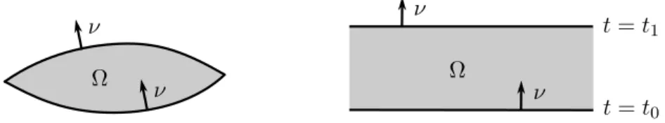
Figure 2. Choice of the space-time region Ω⊂M.
We want to apply Theorem 5.2. Since in this theorem, the set Ω must be compact, we choose it as a lens-shaped region whose boundary is composed of two space-like hypersurfaces (see the left of Figure 2). Considering a sequence of compact sets Ωn
which exhaust the region Ω between two Cauchy surfaces at times t=t0 and t=t1, the surface layer integral (4.24) reduces to the difference of surface layers integrals at times t≈t0 and t≈t1. The detailed analysis (which will be carried out below) gives the following result:
Theorem 5.3. (current conservation) Let (H,F, ρε) be local minimizers of the causal action which describe the Minkowski vacuum (5.4). Considering the limiting procedure explained in Figure 2 and taking the continuum limit, the conservation laws of Theorem 5.2 go over to a linear combination of the probability integrals in every generation. More precisely, there are non-negative constants cβ such that for all u∈H for which ψu is a negative-frequency solution of the Dirac equation, the surface layer integral (4.24) goes over the equation
3
X
β=1
mβcβ ˆ
t=t0
≺ψβu(x)|γ0ψuβ(x)≻d3x=
3
X
β=1
mβcβ ˆ
t=t1
≺ψβu(x)|γ0ψuβ(x)≻d3x . (5.5) The constants cβ depend on properties of the distribution ˆQ in the continuum limit, as will be specified in Definition 5.5 and (5.23) below.
Before coming to the proof, we explain the statement and significance of this the- orem. We first note that the restriction to negative-frequency solutions is needed be- cause the description of positive-frequency solutions involves the so-called mechanism of microscopic mixing which for brevity we cannot address in this paper (see however Remark 8.1 below). Next, we point out that the theorem implies the statement that the functionℓ◦Φ in Theorem 5.2 is continuously differentiable in the continuum limit.
However, this does not necessarily mean that this differentiability statement holds for any local minimizer (H,F, ρε) with regularization. This rather delicate technical point will be discussed in Remark 5.10 below.
Considering Cauchy hyperplanes in (5.5) is indeed no restriction because the theo- rem can be extended immediately to general Cauchy surfaces:
Corollary 5.4. (current conservation on Cauchy surfaces) Let N0,N1 be two Cauchy surfaces in Minkowski space, where N1 lies to the future of N0. Then, under the assumptions of Theorem 5.3, the conservation law of Theorem 5.2 goes over to the conservation law for the current integrals
3
X
β=1
mβcβ ˆ
N0
≺ψβu|/νψβu≻dµN0 =
3
X
β=1
mβcβ ˆ
N1
≺ψuβ|/νψuβ≻dµN1, (5.6) where ν denotes the future-directed normal.
Proof. We choose Ω as the space-time region between the two Cauchy surfaces. Using that the integrand in (4.24) is anti-symmetric in its argumentsxandy, the integration range can be rewritten as
ˆ
Ω
dρ(x) ˆ
M\Ω
dρ(y)
Lκ Φτ(x), y
− Lκ x,Φτ(y)
= ˆ
J∧(N1)
dρ(x) ˆ
J∨(N1)
dρ(y)
Lκ Φτ(x), y
− Lκ x,Φτ(y)
(5.7)
− ˆ
J∧(N0)
dρ(x) ˆ
J∨(N0)
dρ(y)
Lκ Φτ(x), y
− Lκ x,Φτ(y)
, (5.8)
where J∧ and J∨ denote the causal past and causal future, respectively. For ease in notation, we refer to the integrals in (5.7) as a surface layer integral over N1. Thus the surface layer integral in (4.24) is the difference of two surface layer integrals over the Cauchy surfaces N0 and N1.
In order to compute for example the surface layer integral over N0, one chooses Ω as the region between the Cauchy surface N0 and the Cauchy surface t = t0 (for sufficiently small t0; in case that these Cauchy surfaces intersect for every t0, one modifies N0 near the asymptotic end without affecting our results). Applying the conservation law of Theorem 5.2 to this new region Ω, one concludes that the the surface layer integral over N0 coincides with the surface layer integral at time t≈t0. The latter surface layer integral, on the other hand, was computed in Theorem 5.3 to go over to the sum of the probability integrals in (5.5). Finally, the usual current conservation for the Dirac dynamics shows that the the integrals in (5.5) coincide with the surface integral over N0 in (5.6). This concludes the proof.
Using similar arguments, Theorem 5.3 can also be extended to interacting systems (see Remark 5.12 below).
The remainder of this section is devoted to the proof of Theorem 5.3. We first rewrite the causal action principle in terms of the kernel of the fermionic projector (for details see [6,§1.1]). The kernel of the fermionic projectorP(x, y) is defined by
P(x, y) =πxy|Sy : Sy →Sx. (5.9) The closed chainis defined as the product
Axy =P(x, y)P(y, x) : Sx →Sx.
The nontrivial eigenvaluesλxy1 , . . . , λxy of the operatorxycoincide with the eigenvalues of the closed chain. Moreover, it is useful to express P(x, y) in terms of the wave evaluation operator defined by
Ψ(x) : H→Sx, u7→ψu(x) =πxu . (5.10) Namely,
x=−Ψ(x)∗Ψ(x) and P(x, y) =−Ψ(x) Ψ(y)∗.
Our task is to compute the term Lκ(Φτ(x), y) in (4.24) for x, y∈M. The detailed computations in [6,§3.6.1] show that the fermionic projector of the Minkowski vacuum satisfies the EL equations in the continuum limit for κ= 0 (in our setting, this result means that the measures ρε are local minimizers in the sense of Definition 4.3 in the limiting case εց 0). Therefore, we may set κ to zero. Thus our task is to compute
the term L(Φτ(x), y). In preparation, we computeP(Φτ(x), y). To this end, we first note that
Φτ(x)y=UτxU−1τ y=UτΨ(x)∗Ψ(x)U−1τ Ψ(y)∗Ψ(y)
≃Ψ(x)U−1τ Ψ(y)∗Ψ(y)UτΨ(x)∗, (5.11) where in the last line we cyclically commuted the operators and≃means that the op- erators are isospectral (up to irrelevant zeros in the spectrum). Therefore, introducing the notations
Ψτ(x) = Ψ(x)U−1τ : H→Sx (5.12) P Φτ(x), y
=−Ψτ(x) Ψ(y)∗, P y,Φτ(x)
=−Ψ(y) Ψτ(x)∗ (5.13) one sees that the operator product Φτ(x)y is isospectral to the modified closed chain
P Φτ(x), y
P y,Φτ(x)
. (5.14)
Considering the Lagrangian as a function of this modified closed chain, the variation is described in a form suitable for computations.
For clarity, we explain in which sense the kernel of the fermionic projector as given by (5.13) agrees with the abstract definition (5.9),
P Φτ(x), y
=πΦτ(x)y . (5.15)
It is a subtle point that the point Φτ(x) ∈ F depends on τ, so that space-time itself changes. However, when identifying the spin spaceSΦτ(x) with a corresponding spinor space in Minkowski space, the base pointx∈M should be kept fixed. Therefore, the spin spaceSΦτ(x)is to be identified with the spinor spaceSxM. For eachτ, this can be accomplished as explained above. This identification made, the kernel (5.13) indeed agrees with (5.15). The reason why we do not give the details of this construction is that the computation (5.11) already shows that the Lagrangian can be computed with the closed chain (5.14), and this is all we need for what follows.
We now choose A=πhui as the projection on the one-dimensional subspace gener- ated by a vector u∈H and letπhui⊥ be the projection on the orthogonal complement of u. Then
Ψτ(x) = Ψ(x) πhui⊥+e−iτπhui P Φτ(x), y
=−Ψ(x) πhui⊥+e−iτπhui Ψ(y)∗
=P(x, y) + (1−e−iτ) Ψ(x)πhuiΨ(y)∗.
Normalizingusuch that hu|uiH = 1, the last equation can be written in the form that for any χ∈Sy,
P Φτ(x), y
χ=P(x, y)χ+ (1−e−iτ)ψu(x)≺ψu(y)|χ≻y. We now compute the first order variation.
d
dτP Φτ(x), y
τ=0χ=iψu(x)≺ψu(y)|χ≻y =:δP(x, y)χ d
dτP y,Φτ(x)
τ=0 = δP(x, y)∗ (5.16)