Universit¨ at Regensburg Mathematik
Spinors on singular spaces and the topology of causal fermion systems
Felix Finster and Niky Kamran
Preprint Nr. 04/2014
arXiv:1403.7885v1 [math-ph] 31 Mar 2014
CAUSAL FERMION SYSTEMS
FELIX FINSTER AND NIKY KAMRAN APRIL 2014
Abstract. We propose causal fermion systems and Riemannian fermion systems as a framework for describing spinors on singular spaces. The underlying topological structures are introduced and analyzed. The connection to the spin condition in differential topology is worked out. The constructions are illustrated by many simple examples like the Euclidean plane, the two-dimensional Minkowski space, a conical singularity, a lattice system as well as the curvature singularity of the Schwarzschild space-time.
Contents
1. Introduction 2
2. Basic Definitions and Simple Examples 3
3. Topological Structures 8
3.1. A Sheaf 8
3.2. A Topological Vector Bundle 9
3.3. A Bundle over a Topological Manifold 11
3.4. A Bundle over a Differentiable Manifold 14
4. Topological Spinor Bundles 14
4.1. Clifford Sections 14
4.2. Topological Obstructions 17
4.3. The Spin Group 20
4.4. Construction of Bundle Charts 22
4.5. Spin Structures 23
5. Tangent Cone Measures and the Tangential Clifford Section 24
5.1. The Tangent Cone Measures 24
5.2. Construction of a Tangential Clifford Section 28
5.3. Construction of a Spin Structure 30
6. The Topology of Discrete and Singular Fermion Systems 31
7. Examples 33
7.1. The Euclidean Plane 33
7.2. Two-Dimensional Minkowski Space 36
7.3. The Euclidean Plane with Chiral Asymmetry 41
7.4. The Spin Structure of the Euclidean Plane with Chiral Asymmetry 42 7.5. The Spin Structure of Two-Dimensional Minkowski Space 44
8. Spinors on Singular Spaces 48
8.1. Singularities of the Conformal Factor 50
8.2. Genuine Singularities of the Curvature Tensor 54 8.3. The Curvature Singularity of Schwarzschild Space-Time 56
1
8.4. A Lattice System with Non-Trivial Topology 60
References 62
1. Introduction
Causal fermion systems arise in the context of relativistic quantum theory (see the survey articles [10, 14] and the references therein). From the mathematical point of view, they provide a framework for describing generalized space-times (so-called
“quantum space-times”) which do not need to have the structure of a Lorentzian manifold. Nevertheless, many structures of Lorentzian spin geometry (like causality, a distinguished time direction, spinors, connection and curvature) have a generalized meaning in these space-times (cf. [12] or again the survey article [14]). The present work is the first paper in which the topology of causal fermion systems is analyzed.
Moreover, we extend the framework to the Riemannian setting by introducing so-called topological fermion systems. We thus obtain a general setting for describing spinors on singular spaces.
A central idea behind topological fermion systems is to encode the geometry of space (or space-time) in a collection of linear operators on a Hilbert space H. In the smooth setting in which space (or space-time) is a differentiable manifold, one chooses H to be the span of certain spinorial wave functions on the manifold, typically formed of solutions of the Dirac equation. The spatial (or space-time) dependence of the wave functions is then encoded in the so-calledlocal correlation operators, which are bounded linear operators on H. Identifying the points of the manifold with the corresponding local correlation operators, we describe space (or space-time) by a subset of L(H).
Finally, taking the push-forward of the volume measure gives rise to a measure on L(H), the so-calleduniversal measure. This leads to the general setting of topological fermion systems that will be introduced in Definition 2.1 below.
Topological fermion systems also allow for the description of non-smooth geometries in which the underlying space (or space-time) is not a differentiable manifold. This can be understood from the fact that the solutions of a partial differential equation often have better regularity than the coefficients of the PDE they solve. As a consequence, in many situations the wave functions, which are solutions of a geometric PDE, re- main continuous even when the metric or curvature develop singularities. Since we derive all relevant objects (like the spinor bundle and Clifford structures) from the local correlation operators, our framework remains well-defined even in such singular situations. Moreover, we can describe discrete spaces (like lattices) or other highly singular spaces, and our methods endow such spaces with non-trivial topological data.
Our framework is very flexible because there is a lot of freedom in choosing the wave functions inH. This has the advantage that one can describe many different geometric situations by tailoring H in regard to the specific application. It is a main purpose of the present paper to explain how this can be done in different examples. We remark that the framework becomes much more rigid if one assumes that the configurations of wave functions are minimizers of causal variational principles (see [9]) or corresponding Riemannian analogs. The analysis of such variational principles is a separate subject which we cannot enter here. Instead, we refer the interested reader to [19, 2, 13] and the references therein.
The paper is organized as follows. In Section 2 we give the general definition of topological fermion systems and explain in simple examples how such systems can be constructed. In Section 3 we introduce the basic structures inherent to topological fermion systems, starting from the most general singular situation and then specializing in several steps until we end up in the smooth setting. In Section 4 we define so-called topological spinor bundles on a topological manifold and work out the connection to the structures on a usual spin manifold. In Section 5 we address the question of whether a causal fermion system determines a distinguished Clifford structure. In Section 6 we present methods for getting topological information on fermion systems for which the underlying space (or space-time) does not even have the structure of a topological manifold. In Section 7 we illustrate our constructions by the examples of the Euclidean plane and two-dimensional Minkowski space. Section 8 is devoted to examples for spinors on singular spaces: In Section 8.1 we consider singularities of the curvature tensor which can be removed by a conformal transformation. In this case, a rescaling of the spinorial wave functions makes it possible to eliminate the singularity. Section 8.2 treats curvature singularities which cannot be removed by a conformal transformation. In Section 8.3 we describe the curvature singularity of the Schwarzschild black hole. Finally, in Section 8.4 we illustrate the topology of singular spaces in the example of a two-dimensional lattice.
We finally point out that all our constructions are meant to be topological but not differential geometricin the following sense: Starting from a Lorentzian manifold, get- ting into the framework of causal fermion systems makes it necessary to introduce an ultraviolet regularization (for details see [18, Section 4]). This means that the system must be “smeared out” on the microscopic scale. As a consequence, the macroscopic geometry of space-time can be seen only on scales which are larger than the regu- larization length ε. This subtle point is taken care of in the constructions in [12] by working with the notions of “generically time-like separation” and “spin-connectable space-time points.” Moreover, the spin connection in [12] gives a parallel transport along a discrete “chain” of points, and the correspondence to the spinorial Levi-Civita connection is obtained by first taking the limit εց0 and then letting the number of points of the chain tend to infinity (see [12, Theorem 5.12]). Similarly, the Euclidean sign operator (which will be introduced after (4.1) below) depends essentially on the regularization, so that in the constructions in [12] it is handled with care. On the other hand, the ultraviolet regularization can be regarded as a continuous deformation of the geometry for small distances, having no influence on the topology. With this in mind, we here take the point of view that for analyzing topological questions, one can make use of the local behavior of the causal fermion system in an arbitrarily small neigh- borhood of a given space-time point. This leads to different types of constructions which we will explore here. In this way, the topological constructions given in this paper complement the differential geometric constructions in [12] and give a different viewpoint on causal fermion systems.
2. Basic Definitions and Simple Examples
Causal fermion system were first introduced in [14]. Here we give a slightly more general definition and explain it afterwards in a few examples.
Definition 2.1. Given a complex Hilbert space (H,h.|.iH) (the“particle space”) and parametersp,q∈N0withp≤q, we letF⊂L(H) be the set of all self-adjoint operators
on H of finite rank, which (counting with multiplicities) have at most p positive and at most q negative eigenvalues. OnF we are given a positive measureρ (defined on a σ-algebra of subsets ofF), the so-called universal measure. We refer to (H,F, ρ) as a topological fermion system of spin signature (p,q).
In the casep=q, we call (H,F, ρ) acausal fermion systemof spin dimensionn:=p.
If p= 0, we call (H,F, ρ) aRiemannian fermion system of spin dimensionn:=q.
It should be noted that the assumptionp≤qmerely is a convention, because otherwise one may replace F by −F.
A basic feature of topological fermion systems is that the geometry and topology are encoded in terms of linear operators on a Hilbert space. The support of the universal measure ρ, defined by
suppρ={x∈F|ρ(U)>0 for every open neighborhoodU of x} ⊂F,
takes the role of the base space, usually referred to as “space” or “space-time.” This concept is illustrated by the following examples.
Example 2.2. (Dirac spheres)
(i) We choose H = C2 with the canonical scalar product. Moreover, let ˆM = S2⊂R3 and dµ the Lebesgue measure on ˆM. Consider the mapping
F : ˆM →L(H), F(p) = 2
3
X
α=1
pασα+ 11, (2.1) whereσα are the three Pauli matrices
σ1= 0 1
1 0
, σ2=
0 −i i 0
, σ3 =
1 0 0 −1
. (2.2)
For anyp∈S2, the relations tr F(p)
= 2, tr F(p)2
= 10
show that the eigenvalues ofF(p) are equal to 1±2. Hence one eigenvalue is positive and one eigenvalue is negative, so thatF(p)∈Fif we chosep=q= 1.
We introduce the universal measure as the push-forward measure ρ = F∗µ (i.e. ρ(Ω) := µ(F−1(Ω))). Then (H,F, ρ) is a causal fermion system of spin dimension one. The support of ρ is homeomorphic to S2. We refer to this example as a Dirac sphere.
(ii) We again choose H = C2 with the canonical scalar product. Taking two different parametersτ±>1, we introduce the mappings
F±: ˆM →L(H), F(p) =τ±
3
X
α=1
pασα+ 11,
and define the universal measure as the sum of the corresponding push-forward measures,
ρ=F∗+µ+F∗−µ . (2.3)
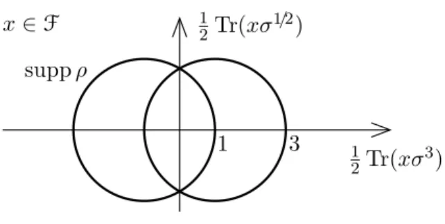
Then (H,F, ρ) is again a causal fermion system of spin dimension one. The support ofρ is homeomorphic to the disjoint union of two spheres.
suppρ
1
2Tr(xσ1/2)
1
2Tr(xσ3) x∈F
1 3
Figure 1. Two intersecting Dirac spheres.
(iii) We consider the mappings
F± : ˆM →L(H), F±(p) = 2
3
X
α=1
pασα+ 11±σ3
and introduce the universal measure again as the sum of the corresponding push-forward measures (2.3). Then (H,F, ρ) is again a causal fermion system of spin dimension one. The support ofρis homeomorphic to two spheres glued together along circles of latitude (see Figure 1). We refer to this example as
two intersecting Dirac spheres. ♦
As already becomes clear in these simple examples, there are usually many ways to realize a topological space as the support of a universal measure. The reason is that a topological fermion system encodes more structures than just the topology, so that prescribing only the topology leaves a lot of freedom to modify all the additional structures.
A particular structure on a topological fermion system is the particle space H.
The vectors in H have the interpretation as the wave functions corresponding to the quantum particles of the physical system (this is also the reason for the name “particle space”). More generally, a basic underlying concept is to encode the geometry and topology in a certain family of functions defined on space or in space-time. This is illustrated in the next examples.
Example 2.3. (Scalar and vector fields on a closed Riemannian manifold)
(i) Let ( ˆM , g) be a smooth compact Riemannian manifold without boundary and ∆ the Laplace-Beltrami operator acting on complex-valued scalar func- tions on ˆM. Then the operator −∆ with domain C∞( ˆM) is an essentially self-adjoint operator onL2( ˆM). It has a purely discrete spectrum lying on the positive real axis. For a given parameter L > 0 we let H be the span of all eigenfunctions corresponding to eigenvalues≤L,
H= rgχ[0,L](−∆)⊂L2( ˆM).
ThenHis a finite-dimensional Hilbert space which, by elliptic regularity theory, consists of smooth functions. Hence, for everyp∈Mˆ the bilinear form (ψ, φ)7→
−ψ(p)φ(p) is well-defined and continuous on H ×H. By the Fr´echet-Riesz theorem, there is a unique linear operator F(p) with the property that
−ψ(p)φ(p) =hψ|F(p)φiL2( ˆM) for allψ, φ∈H. (2.4)
This operator has rank at most one and is negative semi-definite. Varying p, we thus obtain a mappingF : ˆM →F if we choose p= 0 and q= 1. Finally, we define ρ = F∗µ as the push-forward measure of the volume measure (i.e.
ρ(Ω) := µ(F−1(Ω)). Then (H,F, ρ) is a Riemannian fermion system of spin dimension one.
(ii) Let ( ˆM , g) be a smooth compact Riemannian manifold of dimensionk and ∆ the covariant Laplacian on smooth vector fields. Complexifying the vector fields and taking theL2-scalar product
hu|viL2 = Z
Mˆ
gjkujvkdµMˆ ,
the operator−∆ is essentially self-adjoint and has smooth eigenfunctions. We again setH= rgχ[0,L](−∆) and define the operatorF(p)∈L(H) by
−gjkuj(p)vk(p) =hu|F(p)viL2 for all u, v ∈H. (2.5) The operators F(p) are negative semi-definite and have rank at most k. We again introduce the universal measure by ρ = F∗µ. Then (H,F, ρ) is a Rie-
mannian fermion system of spin dimensionk. ♦
In all applications worked out at present, the functions on space or space-time are spinors. In order to get the connection to topological fermion systems, we let ( ˆM , g) be a spin manifold (Riemannian or Lorentzian) and denote the corresponding spinor bundle by SMˆ. Then the spinor space SpMˆ at any point p∈ Mˆ is endowed with an inner product, which we denote by
≺.|.≻p : Sp×Sp →C (2.6)
and refer to as thespin scalar product. Next, we chooseH⊂Γ( ˆM , SMˆ) as a subspace of the continuous sections on ˆM, together with a scalar producth.|.iH(the choice of the scalar product depends on the signature of the metric and the particular application being considered). Then for every p ∈ Mˆ, we can express the scalar product at a point p in terms of the Hilbert space scalar product,
− ≺ψ|φ≻p =hψ|F(p)φiH for allψ, φ∈H. (2.7) According to the Riesz representation theorem, this determines a unique linear oper- ator F(p)∈L(H).
Definition 2.4. The operator F(p) ∈L(H) satisfying (2.7) is referred to as the local correlation operator at the point p∈Mˆ.
By construction, the operator F(p) has finite rank (indeed, its rank is at most the dimension of Sp), and its maximal number of positive and negative eigenvalues is determined by the signature of the spin scalar product. Therefore, we can regardF(p) as an element of F⊂L(H) (for a suitable choice of the spin signature). Varyingp, we obtain a mappingF : ˆM →F. Introducing the universal measure as the push-forward of the volume measuredµ on ˆM, i.e.
ρ(Ω) :=µ(F−1(Ω)),
we obtain a topological fermion system (H,F, ρ). The concept behind taking the push-forward measure is that we want to identify the point p ∈ Mˆ with its local correlation operator F(p)∈F. Likewise, the manifold ˆM should be identified with the
subset F( ˆM) of F. With this in mind, we do not want to work with objects on ˆM, but instead with corresponding objects on F. Apart from giving a different point of view, this procedure makes it possible to extend the notion of the manifold ˆM as well as the objects thereon to a more general setting.
To avoid confusion, we remark that the above-mentioned identification ofpwithF(p) clearly fails if the mapping F is not injective. For this reason, one usually chooses H in such a way that F becomes injective. In certain applications, however, it is indeed preferable to work with a mapping F which is not injective. In this case, all points of ˆM with the same image are identified when forming the topological fermion system.
We will come back to this point in Example 8.3 below.
The simplest setting in which the above construction of topological fermion systems using spinors can be made precise is to choose ˆM as a closed Riemannian manifold:
Example 2.5. (Spinors on a closed Riemannian manifold) Let ( ˆM , g) be a compact Riemannian spin manifold of dimension k ≥ 1. The spinor bundle SMˆ is a vector bundle with fibreSpMˆ ≃Cnwithn= 2[k/2](see for example [31, 21]). The spin scalar product (2.6) is positive definite. On the smooth sections Γ(SMˆ) of the spinor bundle we can thus introduce the scalar product
hψ|φi = Z
Mˆ≺ψ|φ≻pdµ(p), wheredµ=√
detg dkxis the volume measure on ˆM. Forming the completion gives the Hilbert space L2( ˆM , SMˆ). The Dirac operator Dwith domain of definition Γ(SMˆ) is an essentially self-adjoint operator on L2( ˆM , SMˆ). It has a purely discrete spectrum and finite-dimensional eigenspaces (for details see for example [22]). For a given pa- rameter L > 0, we let H be the space spanned by all eigenvectors whose eigenvalues lie in the interval [−L,0],
H= rgχ[−L,0](D)⊂L2( ˆM , SMˆ).
Denoting the restriction of the L2-scalar product to H by h.|.iH, we obtain a finite- dimensional Hilbert space (H,h.|.iH). By elliptic regularity theory, the functions inH are all smooth.
For everyp∈Mˆ we introduce the local correlation operator by (2.7). This operator is negative semi-definite and has rank at most n. Hence F(p) is an element of F according to Definition 2.1 if we choose p = 0 and q = n. Varying p, we obtain a mapping F : ˆM →F. Finally, we define ρ=F∗µ as the push-forward measure of the volume measure. Then (H,F, ρ) is a Riemannian fermion system of spin dimensionn.
This example can readily be extended to an infinite-dimensional particle space by choosing a function f ∈C0(R) and by modifying the above construction to
H= rgf2(D)⊂L2( ˆM , SMˆ)
−≺f(D)ψ|f(D)φ≻p =hψ|F(p)φiH for allψ, φ∈H.
Iff has suitable decay properties at infinity, the operatorf(D) mapsHto the contin- uous functions, so that F(p)∈L(H) is well-defined. We omit the details for brevity.
♦ Examples of causal fermion systems can be obtained similarly starting from a Lorentzian manifold (see [14, Section 1.1], [12, Section 4 and 5] or [18, Section 4]).
In this case, the spaceH has the physical interpretation as describing all the occupied
Dirac quantum states of the system, including the so-called Dirac sea (for the con- nection to physics see [10]). The scalar product on H is typically deduced from the spatial integral over the Dirac current and is thus closely related to the probabilistic interpretation of the Dirac wave function. The fact that Dirac particles are fermions explains the name fermion system. The notion “causal” in a causal fermion system can be understood as follows: Taking the product of two operatorsx, y∈F, we obtain an operator of rank at most p+q. This operator is in general no longer symmetric (because (xy)∗ =yx, and thusxy is symmetric if and only ifxandycommute). Never- theless, we can consider its characteristic polynomial. We denote its non-trivial zeros (counted with algebraic multiplicities) by λxy1 , . . . , λxyp+q. For a Riemannian fermion system, these zeros are all real and non-negative. Namely, in this case the operator−y is positive semi-definite, so that its square root√
−yis well-defined as a positive semi- definite operator. Using that the spectrum is invariant under cyclic permutations, it follows that
xy =−x√
−y√
−y is isospectral to √
−y(−x)√
−y , (2.8) and the last operator product is obviously positive semi-definite. In the casep>0, the operator √
−y no longer exists as a symmetric operator, so that the argument (2.8) breaks down. It turns out that the λxyj will in general be complex, giving rise to the following notion of causality:
Definition 2.6. (causal structure) Two points x, y∈F are calledtimelikeseparated if the non-trivial zeros λxy1 , . . . , λxyp+q of the characteristic polynomial of the operator productxy are are all real. The pointsxand yare said to bespacelikeseparated if all theλxyj are complex and have the same absolute value. In all other cases, the pointsx and y are said to belightlike separated.
3. Topological Structures
In this section we work out the underlying topological structures. We begin with the most general structures and then specialize the setting in several steps. We first recall a few basic notions from [14]. Let (H,F, ρ) be a topological fermion system.
On Fwe consider the topology induced by the operator norm kAk:= sup
kAukH with kukH= 1 .
The base space M (often referred to as “space” or “space-time”) is defined as the support of the universal measure, M := suppρ. On M we consider the topology induced by F. For every x ∈ M we define the spin space Sx by Sx = x(H); it is a subspace ofHof dimension at mostp+q. OnSx we introduce thespin scalar product
≺.|.≻x by
≺ψ|φ≻x =−hψ|xφiH for all ψ, φ∈Sx; (3.1) it is an indefinite inner product of signature (qx, px) withpx ≤pandqx≤q(the minus sign in (3.1) is needed in order to be consistent with the usual sign conventions for Dirac spinors in Minkowski space; for details see [14]).
3.1. A Sheaf. The most general setting in which the topology of a topological fermion system of signature (p,q) can be encoded is a that of a sheaf S on M whose stalks (Sx,≺.|.≻x) are indefinite inner product spaces of signature (qx, px). Although this
setting is too general for most of our constructions (we will mainly work with topolog- ical vector bundles as will be described in Section 3.2 below), we briefly explain how to get the connection to sheaf theory.
For any x ∈ M, we denote the orthogonal projection in H to the spin space Sx
by πx,
πx : H→Sx. (3.2)
Projecting a given vector u∈H to the spin spaces gives the mapping ψu : M →H, x7→πxu∈Sx.
We refer to ψu as thewave function of the occupied state u. For any open subset U ⊂ M, we obtain a corresponding wave function by restriction,
ψu|U : U →H with ψ(x)∈Sx for all x∈U .
We denote the vector space of such wave functions on U by SU. We let S be the mapping which to an open set U assigns the vector space SU. Moreover, for an open subsetV ⊂U we introduce the restriction map as the linear mapping
rVU : SU →SV , ψ7→ψ|V . Obviously, these mappings have the following properties:
(I) IfU is the empty set, then SU ={0}.
(II) The linear map rUU is the identity. If W ⊂V ⊂U, thenrUW =rWV rVU.
This gives the structure of a presheaf of complex vector spaces over the topological space M (see [3] or [28, §I.1.2]). Introducing the corresponding sheaf by taking the direct limits of the vector spacesSU (as outlined for example in [28,§I.1.2]) gives the following structure: We define S as the disjoint union of all spin spaces and π as the projection to the base point,
S:=[˙
x∈M Sx and π : S →M , Sx 7→x .
Everyψ∈SU defines the subset∪x∈Uψ(x)⊂S. OnS we introduce the topology gen- erated by all these subsets. Then the triple (S, π, M) is a sheaf. The stalks (Sx,≺.|.≻x) are indefinite inner product spaces of signature (qx, px).
Now the cohomology groupsHr(M, S),r≥0, with coefficients in a sheaf (as defined for example in [28, §I.2.6]) give topological information on the topological fermion system. For example, globally defined continuous sections are naturally isomorphic to elements of the cohomology group H0(M, S) (see [28, Theorem I.2.6.2]),
Γ(S)≃H0(M, S).
3.2. A Topological Vector Bundle. We now show that under a certain regular- ity assumption (see Definition 3.1), topological fermion systems naturally give rise to topological vector bundles. In preparation, we briefly recall the definition of a topolog- ical vector bundle (see [34, 37]) and set up some notation. LetBandM be topological spaces andπ :B →M a continuous surjective map. Moreover, letY be a complex vec- tor space and G⊂GL(Y) a group acting onY. ThenBis a topological vector bundle with fibreY and structure groupGif every pointx∈M has an open neighborhoodU
equipped with a homeomorphism φU :π−1(U) → U ×Y, called a local trivialization or a bundle chart, such that the diagram
π−1(U) −→φU U ×Y
ց ↓
U
(3.3) commutes, where the projection maps are π and the projection onto the first factor, respectively. Furthermore, on overlaps U ∩V, we have
φU◦φ−V1
{x}×Y =gU V(x), (3.4)
wheregU V :U ∩V →Gis a continuous transition function.
Again setting M = suppρ, we want to construct a topological vector bundle having the spin spaceSx as the fibre at the pointx∈M. To this end, all the spin spaces must have the same dimension and signature, making it necessary to impose the following condition:
Definition 3.1. The topological fermion system is called regular if for allx∈M, the operator x has the maximal possible rank p+q.
Clearly, the topological fermion systems of Example 2.2 are all regular. The topological fermion systems in Examples 2.3 and 2.5 are regular if and only if for everyp∈M, the vectorsψ(p) withψ∈Hspan the fibre atp. We note that most of our constructions can be extended to non-regular topological fermion systems by decomposingMinto subsets on which x has fixed rank and a fixed number of positive and negative eigenvalues.
For clarity, we postpone this decomposition to Section 6 and for now restrict attention to regular topological fermion systems.
We define Bas the set of pairs
B={(x, ψ)|x∈M, ψ∈Sx}
and let π be the projection onto the first component. Moreover, we let (Y,≺.|.≻) be an indefinite inner product space of signature (q,p), and choose G = U(q,p) as the group of unitary transformations on Y. In order to construct the bundle charts, for any given x ∈ M we choose a unitary mapping σ : Sx → Y. By restricting the projection πx, (3.2), to Sy, we obtain the mapping
πx|Sy : Sy →Sx.
In order to compute its adjoint with respect to the spin scalar product (3.1), forψ∈Sx and φ∈Sy we make the computation
≺ψ|πx|Syφ≻x=−hψ|xφiH=−hxψ|φiH =−hπyx ψ|φiH− hy(y|Sy)−1πyx ψ|φiH
=−
(y|Sy)−1πyx ψ yφ
H=≺(y|Sy)−1πyx ψ|φ≻y. Hence
πx|Sy
∗
= (y|Sy)−1πyx . We now introduce the operator
Txy = πx|Sy
πx|Sy
∗
=πx(y|Sy)−1πyx : Sx→Sx.
By construction, this operator is symmetric and Txx = 11. By continuity, there is a neighborhood U of x such that for all y ∈ U, the operator Txy is invertible and has a unique square root ρxy (defined for example by the power series p
Txy =
p11 + (Txy−11) = 11+12(Txy−11)+· · ·). Then the mappingUx,y :=ρ−xy1πx|Sy :Sy →Sx is unitary and depends continuously ony ∈U. We define the bundle chartφU by
φU(y, v) = y,(σ◦Ux,y)(v) .
The commutativity of the diagram (3.3) is clear by construction. The transition func- tions gU V in (3.4) are in G because we are working with unitary mappings of the fibres throughout. We choose the topology on B such that all the bundle charts are homeomorphisms.
Definition 3.2. The topological bundle B → M is referred to as the vector bundle associated to the regular topological fermion system(H,F, ρ), or simply theassociated vector bundle.
3.3. A Bundle over a Topological Manifold. In many applications, M has a manifold structure. This motivates us to specialize our setting by assuming that M is a topological manifold of dimension k ≥ 1 (with or without boundary). From the topological point of view, this is a major simplification which excludes many examples (like the intersecting spheres in Example 2.2 (iii)). The main benefit of this simplifying assumption is that one can choose local coordinates and work with partitions of unity.
As is made precise in the following theorem, these properties ensure that every such bundle can be realized by a topological fermion system. The proof illustrates our concept of encoding the topology of the bundle in a suitable family of sections.
Theorem 3.3. Let X→Mˆ be a bundle over ak-dimensional topological manifoldMˆ, whose fibres are isomorphic to an indefinite inner product space of signature (q,p).
Then there is a regular topological fermion system (H,F, ρ) of signature (p,q) such that the associated vector bundle (see Definition 3.2) is isomorphic to X. If Mˆ is compact, the particle space H can be chosen to be finite-dimensional.
Proof. Let {(xα, Uα)} be an at most countable atlas of ˆM such that the bundle has a trivialization on every Uα. Thus we can choose continuous sections e1α, . . . , ep+qα on Uα which in every point p ∈ Uα form a pseudo-orthonormal basis of the fibre, which we denote by (Sp,≺.|.≻p). Next, we let (Zi)i∈I be an at most countable, locally finite covering of ˆM by relatively compact open subsets, which is subordinate to the atlas {(xα, Uα)} (meaning that for every i ∈ I, there is α = α(i) with Zi ⊂ Uα(i)).
Starting from the sets (Zi)i∈I, we now want to construct non-empty open sets Ωi,Vi
and Wi with the following properties:
(i) The Vi are relatively compact and Ωi ⊂ Vi ⊂⊂ Wi ⊂ Uα(i) for all i ∈ I (where V ⊂⊂W stands for V ⊂V ⊂W).
(ii) The family (Vi)i∈I is a locally finite covering of ˆM.
(iii) Ωi∩Wj =∅for all i6=j.
To this end, we proceed inductively in the index i. If the index set I is finite, we denote it byI ={1, . . . , K}withK∈N. IfI is infinite, we setI =N,K=∞and use the notation Z1∪ · · · ∪ZK ≡ ∪i∈NZi. We letW1 =Z1 and setA1 =∁(Z2∪ · · · ∪ZK).
Then A1 is a closed (possibly empty) set contained inZ1. We choose non-empty open sets Ω1 and V1 such that A1 ⊂ Ω1 ⊂⊂ V1 ⊂⊂ W1. For the induction step, assume that Ωi,Vi andWi have already been constructed for somei. We set
Wi+1=Zi+1\(Ω1∪ · · · ∪Ωi) (3.5) Ai+1=∁ V1∪ · · · ∪Vi∪Zi+2∪ · · · ∪ZK
. (3.6)
ThenAi+1is a closed subset ofWi+1. IfWi+1is empty, we skip this step and increasei.
Otherwise, we choose non-empty open sets Ωi+1 and Vi+1 such that
Ai+1⊂Ωi+1⊂⊂Vi+1 ⊂⊂Wi+1. (3.7) Let us verify that the resulting sets Ωi,ViandWi really have the above properties (i)–
(iii). The properties (i) and (iii) are obvious by construction. To prove (ii), letp∈Mˆ. Since (Zi)i∈I is a locally finite covering, there is an index i∈ I such that p 6∈Zj for all j > i+ 2. But then one sees from (3.6) and (3.7) that p ∈ V1 ∪ · · · ∪Vi+1. We conclude that (i)–(iii) hold.
Next, as in the usual construction of the partition of unity, we choose non-negative continuous functions ηi ∈ C0( ˆM ,R+
0) with ηi|Vi ≡ 1, ηi|Wi\Vi < 1 and suppηi ⊂ Wi. We consider the family of compactly supported continuous sections
ηieℓα(i) and ηixjα(i)eℓα(i), (3.8) where i ∈ I, ℓ = 1, . . . ,p+q and j = 1, . . . , k. Let us verify that these sections are linearly independent. Thus suppose that a linear combination of these functions vanishes. Restricting the functions to Ωi, by property (iii) all the functions with j6=i drop out. Thus it remains to show that for any fixedi, the sections in (3.8) restricted to Ωiare linearly independent. But this follows immediately from the fact that theeℓα(i) are linearly independent at everyp∈Ωi, and that the coordinate functions of the chart are linearly independent and not locally constant.
We let H0 be the vector space spanned by the family of sections (3.8). In order to introduce a scalar product, we represent a functionφ∈H0 locally in components,
φ(p) =
k
X
ℓ=1
φℓ xα(p)
eℓα(i) forp∈Uα, and introduce the L2-scalar product
hφ|ψiH=X
i∈I
Z
xα(i)(Uα(i))
ηi(x)
k
X
ℓ=1
φℓ(x)ψℓ(x)dkx (3.9) (thus we define the eℓα(i) to be orthonormal and take the measure as a weighted sum of the Lebesgue measures in the charts). This scalar product is well-defined and finite because the functions in H0 all have compact support and because the sum in (3.9) is locally finite. Moreover, it is clear from our construction that H0 is locally finite- dimensional in the sense that for any compactK ⊂Mˆ, the function space
H|K :={ψ|K withψ∈H0} is finite-dimensional.
Let us analyze whether (H0,h.|.iH) is complete. Thus let φn ∈ H0 be a Cauchy sequence. Then for every compact K ⊂M, the functionsˆ φn|K are also a L2-Cauchy sequence. Since the space H|K is finite-dimensional, it follows immediately that the sequenceφn|K converges inH|K. However, the functionsφnneed not converge globally inH0. For this reason, we introduce H as the completion ofH0,
H:=H0h.|.iH.
Clearly, (H,h.|.iH) is a Hilbert space. Moreover, the functions in H are again locally finite and H|K =H0|K. In particular, the functions in H are all continuous. If ˆM is compact, then H is obviously finite-dimensional.
For any p∈Mˆ, we define the local correlation operatorF(p) again by (2.7). Since the functions (3.8) restricted to any pointpspan the fibre, the operatorF(p) has max- imal rankp+q. Similar as in (3.9), we choose on ˆM the measuredµ=P
i∈Iηi(x)dkx.
Introducing the universal measure as the push-forward measureρ =F∗(µ), we obtain a regular topological fermion system (H,F, ρ) of spin signature (p,q).
It remains to prove that ˆM is homeomorphic to M := suppρ ⊂ F, and that the bundleB →M is homeomorphic to the bundleX→M. First, sinceˆ His locally finite- dimensional and the functions in H are all continuous, the mapping F : ˆM → F is continuous. As a consequence, the pre-image of any open neighborhood of a pointq ∈ F( ˆM) is a non-zero open subset of ˆM, and thus has non-zeroµ-measure. This implies that F( ˆM)⊂suppρ. Thus it suffices to show that the mapping
F : ˆM →suppρ⊂F is a homeomorphism. (3.10) In order to show that F is injective, let p, q ∈ Mˆ with F(p) = F(q). Then in view of (2.7), we know that
≺φ(p)|ψ(p)≻p=≺φ(q)|ψ(q)≻q for all φ, ψ∈H. (3.11) Evaluating these relations for the functions ηieℓα(i) in (3.8), we conclude thatηi(p) = ηi(q) for alli. As a consequence, we can choose the index isuch thatp, q∈Vi. Next, evaluating (3.11) forφ=ηieℓα(i)andψ=ηixjα(i)eℓα(i), we conclude thatxjα(i)(p) =xjα(i) for all j= 1, . . . , k, implying thatp=q.
We next prove that the mapping (3.10) is open: For given p∈Mˆ we chooseisuch that p ∈ Vi. We let Hi ⊂ H be the subspace spanned by the functions in (3.8), and denote the orthogonal projection to Hi byπHi. Then for anyq ∈Mˆ,
kF(p)−F(q)kL(H)= sup
u∈H,kuk=1hu|(F(p)−F(q))ui
≥ sup
u∈Hi,kuk=1hu|(F(p)−F(q))ui=kπHi(F(p)−F(q))πHikL(H)
≥c
ηieℓα(i)
(F(p)−F(q))ηieℓα(i) +c
k
X
j=1
ηieℓα(i)
(F(p)−F(q))ηixjα(i)eℓα(i)
=c
ηi(p)2−ηi(q)2 +c
k
X
j=1
ηi(p)2xjα(i)(p)−ηi(q)2xjα(i)(q) ,
where the constant c =c(i) >0 depends on the scalar products of the vectors in Hi (here we use that on a finite-dimensional vector space all norms are equivalent). If the left side of this inequality tends to zero, then η(q)→ η(p) = 1 and, so that q lies in Wi. Moreover, xji(q)→ xj(p), implying that q→ p. Hence F−1 is continuous. We conclude that F : ˆM →M is a homeomorphism.
Finally, we show that the corresponding bundlesX → Mˆ and B →M are homeo- morphic. First, any function ψ in (3.8) is a continuous section of the bundleX →M. Identifying ψ with a vector in H, the mapping x 7→πxψ defines a continuous section
in B → M. This identification of sections can be used to construct a homeomor- phism of bundles: For any u ∈ Xp we choose a function ψ ∈ H0 with ψ(p) = u.
Setting x = F(p), we obtain the vector πxψ ∈ Sx. As is obvious by construction, the mapping u 7→ πxψ does not depend on the choice of ψ and thus defines a map- ping X → B. This mapping is compatible with the projections. Moreover, it is a bijection of the fibres which depends continuously on the base point. Thus it defines
a homeomorphism of the bundles.
In the setting of a topological manifold, it is reasonable to assume that ρ should be a continuous measure in the sense that ρ({x}) = 0 for all x ∈M. However, this assumption will not be needed in this paper.
3.4. A Bundle over a Differentiable Manifold. In many situations, M is even a differentiable manifold (again of dimension k ≥ 1). We will assume that M is differentiable whenever the tangent space or the tangent bundle are needed in our constructions (more precisely, in Section 4.5, Section 5.3 and some of our examples).
In the differentiable setting, it is natural to assume that the universal measure is compatible with the differentiable structure in the following way: First, we always assume that the injection
M ֒→F⊂L(H) is Fr´echet differentiable. (3.12) This assumption makes it possible to identify tangent vectors on M with tangent vectors in F. Moreover, it is a reasonable assumption that the measure ρ should be absolutely continuous with respect to the Lebesgue measure in a chart.
4. Topological Spinor Bundles
The vector bundle associated to a regular topological fermion system (see Defini- tion 3.2) is reminiscent of a spinor bundle. In particular, a section ψ of this bundle takes values in the spin spaces, ψ(x) ∈ Sx, and can thus be regarded as a spinorial wave function. However, important structures of a spinor bundle like Clifford mul- tiplication are still missing. We shall now introduce these additional structures and analyze the topological obstructions to their existence. This will make it possible to interpret the vector bundles constructed in Sections 3.2 and 3.3 above as true spinor bundles corresponding in the classical sense of the term to bundles of Clifford algebras and representations of the spin group. We shall see that the topological conditions which the topological fermion system will be required to satisfy (see Theorem 4.5 below) are independent of the standard topological condition for the existence of a spin structure, as expressed by the vanishing of the second Stiefel-Whitney class (see Section 4.5). Thus there are conditions for the existence of spin structures that are specific to topological fermion systems.
4.1. Clifford Sections. In this section we only assume that the topological fermion system is regular (see Definition 3.1). We denote the space of symmetric linear oper- ators on Sx by Symm(Sx) ⊂ L(Sx). Then for any x ∈ M, the operator (−x) on H has q positive and p negative eigenvalues. We denote its positive and negative spec- tral subspaces by Sx+ and Sx−, respectively. In view of (3.1), these subspaces are also orthogonal with respect to the spin scalar product,
Sx =Sx+⊕Sx−. (4.1)
Moreover, we introduce theEuclidean sign operator sx as a symmetric operator on Sx whose eigenspaces corresponding to the eigenvalues ±1 are the spaces Sx+ and S−x, respectively. Clearly, for a Riemannian fermion system the Euclidean sign operator is the identity on Sx.
In order to get a connection to the usual Clifford multiplication, we need the notions of a Clifford subspace and a Clifford extension. These notions were first introduced in [12] for causal fermion systems of spin dimension two. We now extend them to general spin dimension.
Definition 4.1. A subspace K ⊂Symm(Sx) is called a Clifford subspace of signa- ture (r, s) at the point x (with r, s∈N) if the following conditions hold:
(i) For any u, v ∈K, the anti-commutator {u, v} ≡uv+vu is a multiple of the identity on Sx.
(ii) The bilinear formh., .i on K defined by 1
2{u, v}=hu, vi11 for all u, v∈K (4.2) is non-degenerate and has signature (r, s).
We denote the set of Clifford subspaces of signature (r, s) at x by K(r,s)x .
In the settingp=qof causal fermion systems, a useful method for constructing Clifford subspaces is to begin with the Euclidean sign operatorsx and to add operators which anti-commute with it. This gives rise to the so-called Clifford extensions.
Definition 4.2. On a causal fermion system, a Clifford subspace K which contains the Euclidean sign operator is referred to as a Clifford extension (of the Euclidean sign operator sx).
Lemma 4.3. A Clifford extension of dimension mhas Lorentzian signature(1, m−1).
Proof. We choose an orthonormal basis (sx, e1, . . . , em−1) of the Clifford extensionK.
Choosing an orthonormal eigenvector basis of sx, we can represent the Euclidean sign operator by the matrix
sx =
11 0 0 −11
.
Due to the anti-commutation relations, in this basis the operators ej have the matrix representations
ej =
0 a∗j aj 0
and a∗j =−a†j
(where the dagger denotes transposition and complex conjugation). Hence (e2j) =− a†jaj 0
0 aja†j
! .
Noting that this matrix is negative definite, we obtain the claim.
We denote the Clifford extensions of signature (1, r) by Ksxx,r.
In order to introduce global sections of the Clifford algebra, we let Sm be the set of m-dimensional subspaces of L(H) endowed with the topology coming from the metric
d(K, L) = sup
u∈K,kuk=1
vinf∈Lku−vk + sup
v∈L,kvk=1
uinf∈Kku−vk.
Moreover, we let CℓM be a continuous mapping which to every space-time point as- sociates a Clifford subspace,
CℓM : M →Sr+s, x7→Cℓx∈ K(r,s)x . (4.3) We refer toCℓM as aClifford sectionof signature (r, s). It is asection of Clifford extensions if Cℓx ∈ Ksxx,r for allx∈M.
Choosing a Clifford section is the main step for getting into the setting in which the elements of Sx can be interpreted as spinors. In the remainder of Section 4, we shall work out this setting in more detail. More precisely, in Section 4.2 we shall analyze topological obstructions for the existence of Clifford sections. In Section 4.3 we will construct the analogs of the usual Pin and Spin groups. In Section 4.4 spinors, spinor bases and bundle charts for spinor bundles will be defined. Finally, in Section 4.5 we will introduce spin structures which associate a tangent vector on a differentiable manifold to a vector in the corresponding Clifford subspace. Altogether, these con- structions extend the usual structures of spin geometry to the framework of topological fermion systems.
Before entering the detailed analysis, we now give a brief overview of the different situations of interest. First, recall that regular topological fermion systems (H,F, ρ) on a topological manifoldM = suppρ are distinguished by their spin signature (p,q) and the dimension k of M, which can be chosen independently. When choosing Clifford subspaces or Clifford sections, the signature (r, s) of the Clifford subspace gives addi- tional parameters. If one considers causal fermion systems and Clifford extensions, the signature of the spin scalar product is (n, n) and the signature of the Clifford subspace is (1, m−1), leaving us with two parametersn and m to describe the signatures. In usual spin geometry, the dimension of the Clifford subspace always coincides with the dimension of the manifold, i.e.
k=r+s(in general) or k=m (for Clifford extensions). (4.4) In our setting, these relations are needed if we want to introduce Clifford multiplication with tangent vectors, because then one needs to identify the tangent spaceTxM with the corresponding Clifford subspaceCℓx. This construction will be given in Section 4.5 below. At the present stage, there is no need to impose the relations (4.4). On the contrary, for the sake of having more flexibility it is preferable to carefully distinguish the dimension of the manifold from the dimension of the Clifford subspace and to treat these dimensions as independent parameters.
More specifically, in the case of spin signature (2,2) and Clifford extensions of di- mension m = 4, one can get the correspondence to Dirac spinors on a Lorentzian manifold. In this case, the corresponding geometric structures are worked out in [12].
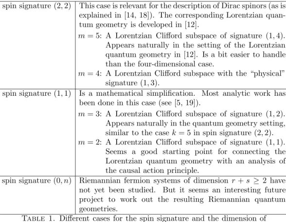
Indeed, most of the constructions in [12] apply just as well to the case m= 5. In order to model the interactions of the standard model, one should increase the spin signature to (2ℓ,2ℓ) with ℓ = 2 (to get the weak interaction and gravity [11]) or ℓ= 8 (to also include the strong interaction [6]). These cases of higher spin signature have not yet been studied systematically. If the spin signature is decreased to (1,1), the spin spaces are two-dimensional, making it impossible to represent Dirac spinors. But one can describe Pauli-like spinors in dimensions m = 1, 2 or 3. In these lower-dimensional situations, the geometric constructions of [12] simplify considerably. This gives hope that it should be possible to connect the geometric notions to the methods and notions arising in the analysis of causal variational principles (see [9, 19, 2, 13]). We consider
spin signature (2,2) This case is relevant for the description of Dirac spinors (as is explained in [14, 18]). The corresponding Lorentzian quan- tum geometry is developed in [12].
m= 5: A Lorentzian Clifford subspace of signature (1,4).
Appears naturally in the setting of the Lorentzian quantum geometry in [12]. Is a bit easier to handle than the four-dimensional case.
m= 4: A Lorentzian Clifford subspace with the “physical”
signature (1,3).
spin signature (1,1) Is a mathematical simplification. Most analytic work has been done in this case (see [5, 19]).
m= 3: A Lorentzian Clifford subspace of signature (1,2).
Appears naturally in the quantum geometry setting, similar to the case k= 5 in spin signature (2,2).
m= 2: A Lorentzian Clifford subspace of signature (1,1).
Seems a good starting point for connecting the Lorentzian quantum geometry with an analysis of the causal action principle.
spin signature (0, n) Riemannian fermion systems of dimension r+s ≥ 2 have not yet been studied. But it seems an interesting future project to work out the resulting Riemannian quantum geometries.
Table 1. Different cases for the spin signature and the dimension of the Clifford subspaces.
this to be a promising starting point for future research. The study of Riemannian fermion systems is also a project for the future. The different cases are summarized in Table 1.
4.2. Topological Obstructions. The goal of this section is to determine topologi- cal obstructions to the existence of Clifford sections. We shall see that there is an interesting interplay between the conditions that need to be satisfied for the existence of Clifford sections and the usual obstructions to the existence of spin structures on a differentiable manifold as expressed by the usual vanishing of the second Stiefel- Whitney class. The connection between these different conditions will become clear in Section 4.5 below. For the moment, the question whether a Clifford section exists is independent of the usual topological spin condition. This illustrated by the following example which shows that a smooth manifold may fail to admit a section of Clifford extensions even if its tangent bundle is spin.
Example 4.4. (Non-existence of Clifford sections on the Dirac sphere) We return to the Dirac sphere of Example 2.2 (i). At a point x = F(p) ∈ suppρ, the spin scalar product (3.1) takes the form
≺.|.≻x=−h., F(p).iC2 .
By definition, the Euclidean sign operator has the same eigenspaces as (2.1) with eigenvalues ±1, so that
sx =−p·σ
(where the dot is a short notation for the sum over the products of components).
We now choose a convenient parametrization of the space Symm(Sx). Let|F(p)|be the absolute value of the operator F(p), i.e. by (2.1)
|F(p)|=
3
X
α=1
pασα+ 2 11≡p·σ+ 2 11.
Writing a linear operator in the form A = |F(p)|−1B|F(p)|, a direct computation shows that Ais symmetric with respect to the inner product≺.|.≻p if and only ifB is symmetric with respect to the inner producth., p·σ.iC2. Moreover, a short computation yields
Symm(Sx) =
|F(p)|−1(α11 +β p·σ+i u·σ)|F(p)|
with α, β ∈R, u∈R3 and u⊥p . (4.5) In order to obtain a two-dimensional Clifford extension at a point p, we need to choose an operator in Symm(Sx) which anti-commutes with sx and whose square equals −11. A short computation using (4.5) yields
Kxsx,1 =n
span sx, i|F(p)|−1u·σ|F(p)|
u∈S2 ⊂R3 withu⊥po .
We conclude that a two-dimensional section of Clifford extensionsamounts to finding a tangent unit vector field on the sphere. However, such a vector field does not exist by the well-known “hairy ball theorem”.
The existence of general Clifford sections (which may not necessarily be Clifford extensions) depends on the dimension and signature. A three-dimensional Clifford section necessarily has signature (1,2). There is the unique Clifford section
Cℓx=
|F(p)|−1(β p·σ+i u·σ)|F(p)|with α, β∈R, u∈R3 and u⊥p , which is also a section of Clifford extensions. Two-dimensional Clifford sections exist in signature (0,2), like for example
Cℓx =
|F(p)|−1(i u·σ)|F(p)|with u∈R3 and u⊥p .
By applying a unitary transformation Cℓx → U(p)CℓxU(p)−1, where U is a continu- ous family of unitary transformations U(p) ∈ U(Sx), one can construct many other Clifford sections of signature (0,2). In signature (1,1), however, no Clifford section exists, as the following argument shows: Suppose that Cℓx were a Clifford section of signature (1,1). Choosing a positive definite vector unit vector v inCℓx, it is of the form
v=|F(p)|−1 ±cosh(α)p·σ+isinh(α)u·σ
|F(p)|
with α ∈R, and u⊥p. Varying p, by continuity we can always choose the plus sign to obtain a global section v(p). A unit vector win the orthogonal complement ofv(p) inCℓx is of the form
w=|F(p)|−1 β p·σ+i t·σ
|F(p)|
withβ ∈R, and where the vector tis tangential toS2 and has length at least one. In this way, the orthogonal complement of v(p) determines a continuous family of one- dimensional subspaces of the tangent space of S2, in contradiction to the “hairy ball
theorem.” ♦
This example illustrates that sections of Clifford extensions do not exist on all topo- logical manifolds. Obstructions to the existence of Clifford sections can be derived for a fairly general class of topological manifolds from classical results on obstructions to the existence of continuous cross-sections of topological fiber bundles over cell com- plexes [37]. In order to apply these results, we will need to assume that our topological manifoldM is homeomorphic to afinite cell complex. This will be the case for example if M is a compact topological manifold [30]. Let us recall the following result from [37, Corollary 34.4] which gives the topological obstructions to the existence of continuous cross sections:
Theorem 4.5. Let B be a bundle over a finite cell complex K, such that for all 1≤q ≤dimK, the fibre Y is (q−1)-simple. If
Hq K,B(πq−1(Y))
= 0 ∀ 1≤q≤dimK , (4.6)
then B admits a continuous cross-section.
To explain the notions in this theorem, we first recall that a path-connected space Y is q-simple if the action of π1(Y, y0) on the qth homotopy group πq(Y, y0) is trivial for some base point y0 ∈ y (and therefore all base points). The assumption that the fibre Y is (q −1)-simple implies that the homotopy group πq−1(Y) is defined independent of a base point. Finally, B(πq−1(Y)) denotes the bundle over K whose fibre at a pointx∈Kis the homotopy groupπq−1of the corresponding fibreB(x)≃Y. For the Clifford extensions that we will consider in this paper, the fibres Y are isomorphic to Lie subgroups of SU(1,1), SU(2,2) or SU(n), and are thereforeq-simple, since topological groups areq-simple for allq (see [36, Theorem 7.3.9] or [25, page 281, Section 3C]). Therefore, the only obstructions to the existence of Clifford extensions are given by the cohomological conditions (4.6).
We now formulate these conditions explicitly for causal fermion systems in the cases in which M is a topological manifold Mk of dimension k and the fibre Y is the set of Clifford extensions of dimension m according to Table 1. In the case m = 5, the fibreY in spin dimensionn= 2 is isomorphic to the circle groupS1 which acts simply transitively on the set of Clifford extensions (see [12, Corollary3.7 and Lemma 3.8]).
We thus obtain
π0(Y) = 0, π1(Y) =Z, πn(Y) = 0 ∀n≥2, (4.7) and the obstructions (4.6) reduce to
H2(Mk,Z) = 0. (4.8)
Next, in the casem= 4 of a four-dimensional Clifford extension, the fibreY (again in spin dimension n= 2) is isomorphic to the productS1×SO(4,R), so that
π0(Y) = 0, π1(Y) =Z×Z2, π2(Y) = 0, π3(Y) =Z×Z. (4.9) The cohomological obstructions (4.6) to the existence of a Clifford extension are there- fore given by
H2(Mk,Z×Z2) = 0 and H4(Mk,Z×Z) = 0. (4.10) The remaining cases of interest are m = 2 and 3, with the spin dimension n taken to be equal to one. For m = 3, the fibre Y reduces to a point, giving no topological