An Adaptive Approach to Forecasting Three Key Macroeconomic Variables for Transitional China

(1)

S F B

XXX

E C O N O M I C

R I S K

B E R L I N

SFB 649 Discussion Paper 2015-023

An Adaptive Approach to Forecasting Three Key

Macroeconomic Variables for Transitional China

Linlin Niu*

Xiu Xu*

Ying Chen**

*Xiamen University, People’s Republic of China

**National University of Singapore, Republic of Singapore

This research was supported by the Deutsche

Forschungsgemeinschaft through the SFB 649 "Economic Risk".

http://sfb649.wiwi.hu-berlin.de ISSN 1860-5664

SFB

6 4 9

E C O N O M I C

R I S K

B E R L I N

(2)

An Adaptive Approach to Forecasting Three Key Macroeconomic Variables for Transitional China

Linlin Niu^a,b,c ^∗ Xiu Xu^a† Ying Chen^d

aWang Yanan Institute for Studies in Economics (WISE), Xiamen University, China

bBank of Finland, Institute for Economies in Transition (BOFIT)

cKey Laboratory of Econometrics (Xiamen University), Ministry of Education, China

dDepartment of Statistics & Applied Probability, National University of Singapore

Abstract

We propose the use of a local autoregressive (LAR) model for adaptive estimation and forecasting of three of China’s key macroeconomic variables: GDP growth, inflation and the 7-day interbank lending rate. The approach takes into account possible structural changes in the data-generating process to select a local homogeneous interval for model estimation, and is particularly well-suited to a transition economy experienc- ing ongoing shifts in policy and structural adjustment. Our results indicate that the proposed method outperforms alternative models and forecast methods, especially for forecast horizons of 3 to 12 months. Our 1-quarter ahead adaptive forecasts even match the performance of the well-known CMRC Langrun survey forecast. The selected homogeneous intervals indicate gradual changes in growth of industrial production driven by constant evolution of the real economy in China, as well as abrupt changes in interest- rate and inflation dynamics that capture monetary policy shifts.

Keywords: Chinese economy, local parametric models, forecasting JEL Classification: E43, E47

∗Linlin Niu acknowledges the support of the Natural Science Foundation of China (Grant No. 70903053 and Grant No. 71273007), and thanks BOFIT Visiting Researcher Programme for hospitality during her research stay at BOFIT.

†Corresponding author. Xiu Xu, Rm A306, Economics Building, Xiamen University, Xiamen, 361005, Fujian, China. Email: xiu.xu@stu.xmu.edu.cn. Phone: +86-592-2182839. Fax: +86-592-2187708. Xiu Xu thanks the support by the Deutsche Forschungsgemeinschaft through the International Research Training Group IRTG 1792 "High Dimensional Non Stationary Time Series" and the SFB 649 Economic Risk.

(3)

1 Introduction

A large body of literature focuses on forecasting important macroeconomic variables such as inflation rate and GDP growth, yet accurate prediction of these variables remains elusive for economists and policymakers (Bräuning and Koopman,2013;Clements and Hendry,2008;

De Gooijer and Hyndman,2006). One of the biggest challenges lies in the irregular, unantic- ipated, and sometimes large, shifts in economic activities that lead to parameter instabilities in parameterized models (D’Agostino et al., 2013; Stock and Watson, 1999, 2007). As a result, the forecasting performance of econometric models may vary dramatically across different sample periods (Rossi and Sekhposyan, 2010). The task of accurately forecasting major macroeconomic variables become even more daunting for transition economies such as China, Russia and countries in eastern Europe as they suffer from limited effective data length compared to developed economies, as well as frequent structural changes and evolving policies.

China has seen several decades of rapid economic growth and remarkable economic achievements since the launch of its reforms in 1978. GDP growth averaged 9.8% a year from 1978 to 2013, and China surpassed Japan as the world’s second largest economy in 2009.

This extraordinary performance reflects two simultaneous trends: China’s gradual transition from a planned economy to its current socialist market model, and the active adoption of modern technology and management practices. During its transition process, China has experienced major policy regime shifts and vast structural reforms. Notable reforms include the agricultural reform that introduced household responsibility system in 1981; the reform of state-owned enterprises (SOEs) in the 1980s; decentralization of decision-making and the rise of township enterprises in the mid-1980s; the marketization of prices in 1992; the fiscal and tax system reform in 1994 to broaden the tax base and decentralize the tax collection power; the financial system reform in 1999; entry into the WTO in 2002; and the reform in exchange-rate regime in 2005 (Naughton,2007;Lin,2013;Chow,2015). Such policy adjust- ments can affect economic structures, pricing mechanisms, degrees of market competition and the decision-making powers of agents in ways that impact aggregate economic variables such as GDP growth, the inflation rate and key interest rates. Thus, the dynamics of these variables in a transition economy context need to reflect these structural changes to achieve a modicum of forecasting accuracy.

The literature provides many fruitful studies in forecasting macroeconomic variables, ranging from parsimonious time-series models and macro-theoretical based models such as the Philips curve model to structural VAR and factor-augmented VAR models (Stock and Watson,1999, 2002a,b; Forni et al.,2000, 2003; Bai and Ng,2002, 2008). To address the issue of parameter instability, many models include features of long memory or structural breaks (Clements and Hendry,1996;Banerjee et al.,2008; Stock and Watson, 2009;Clark

(4)

and McCracken,2010;Geweke and Jiang,2011;D’Agostino et al.,2013). Even so, complex econometric models often fail to outperform simple time-series models or forecasts based on survey data (Ang et al.,2007;Stock and Watson,2008;Belmonte and Koop,2014). The factor-augmented VAR model, for example, hinges on the effective selection of factors and tends to perform poorly in out-of-sample forecasting due to potential structural changes of the factors. Predicting local shifts in factors can also present computationally non-trivial challenges (Castle et al.,2013).

Moreover, most of the above-mentioned methodological research work on predicting macroeconomic time series focuses on developed countries. Existing macroeconomic forecasts for developing countries, especially transition economies, tend to be empirical applications and comparisons of the aforementioned forecast models and approaches. For example, Krkoska and Teksoz(2007) make a comprehensive analysis of the forecast accuracy of output growth for transition countries in central and eastern Europe and former Soviet Republics based on the performance of forecasts produced by the European Bank for Reconstruction and Development (EBRD). Ahumada and Garegnani (2012) estimate Argentinian money demand with an equilibrium-correction model of monetary aggregate M2 and compare the performance of the model with alternative forecasting approaches, including VAR, naive models and pooling of different forecasts. Notably, studies of systematic forecasting in transition economies largely overlook transition effects.

Forecasting macroeconomic indicators of transition economies has two notable features.

First, structural changes due to policy and regime shifts occur much more often than in developed economies. Second, available data tend to be far more limited and of poorer quality than in developed economies. This paper takes these two features into consideration by incorporating an adaptive approach for estimating and forecasting three key macroeconomic variables for China with a local autoregressive (LAR) model.

Chen, Härdle and Pigorsch (2010) initially propose a LAR model to forecast realized volatilities in order to identify typical long-memory patterns of financial time series. Since parameter instability of stationary processes can produce spurious long-memory phenomena, the authors adopt a strategy of nesting local homogenous intervals with relatively stable parameters into a global process. Through Monte Carlo experiments and empirical out-of- sample forecasting for the potentially nonstationary time series, their LAR method beats popular alternative models when dynamic selection of the homogeneous sample interval is used with a parsimonious local AR(1) model. Chen and Niu (2014) further apply the local adaptive approach to forecast the term structure of US interest rates. Their method substantially outperforms alternative term-structure methods in forecasts with 3- to 12- month horizons. The approach is shown to capture structural changes of the time series quite well, and commonly identified interval endings are in line with major policy changes

(5)

or economic recessions.

Given the above-mentioned feature of transition economies, the LAR model appears particularly suitable for forecasting key macroeconomic variables in situations of limited sample length or vulnerability to structural breaks. Recent successful applications of the adaptive approach include Härdle et al. (2014a) and Härdle et al. (2014b) in forecasting trading volumes and order flow in financial markets.

Based on adaptively identified homogeneous intervals, we directly utilize a parsimonious LAR(1) model to forecast China’s macroeconomic variables. Our three selected variables are the growth rate of industrial production (IP growth) as a proxy for real GDP growth, the CPI inflation rate as a representative for nominal variables, and the 7-day China Interbank Offered Rate (Chibor, i.e. National Interbank Offered Rate) as a money market indicator.

For forecast comparison, we choose popular forecast models with predetermined estimation windows as alternatives. For inflation, we follow Ang et al. (2007), employing a Philips curve model, a time-series AR model, an interest-rate term-structure model and a combined model. For IP growth, we draw on the idea of selecting alternative models suggested by Stock and Watson(2002a), choosing as our alternative models an AR model, macroeconomic models with various factors, a random-walk model and a combined model. For interest rate, we choose AR and random-walk models as alternatives.

The literature repeatedly points to the difficulty of beating survey forecasts (e.g. Ang et al., 2007; Belmonte and Koop, 2014), so we compare our forecast results against the well-recognized China Macroeconomic Research Center (CMRC) Langrun survey forecast.

Our LAR model substantially outperforms alternative models with predetermined regression windows in 3- to 12-month ahead forecasts. For example, the forecast root mean squared errors (RMSE) of the 12-month ahead LAR forecast has been reduced by about 30 % compared to alternative models. Our 1-quarter ahead LAR forecasts are as good as CMRC survey forecasts.

The LAR identified homogeneous intervals further provide useful information on monitoring and understanding China’s economic dynamics in real time. We find from the identified homogenous intervals several abrupt changes in inflation and interest rate that are in line with major reforms of monetary policy and institutions. For IP growth, in contrast, only gradual changes in homogenous intervals are detected. This likely reflects gradual transition of the real economy, echoing the immensity and scope of China’s economic reforms.

The rest of the paper is organized as follows. Section 2 describes the adaptive model.

Section 3 presents our data, the forecast procedure and alternative models for comparison.

Section 4 presents the forecast results and comparison with detailed discussion. Section 5 concludes.

(6)

2 LAR-based adaptive modeling and forecasting

We followChen, Härdle and Pigorsch(2010) to model each of the macroeconomic time series as an LAR(1) model. The time series in an identified homogenous interval can be modeled locally as a typical AR model with approximately constant parameters. The LAR treats the parameters globally in a time-varying manner. Chen, Härdle and Pigorsch(2010) show that a simple LAR model can outperform GARCH models and other popular volatility models when applied to forecasting realized volatility. Chen and Niu (2014) extend their local autoregressive model to incorporate exogenous variables (LARX model). The LARX model effectively forecasts yield factors and outperforms typical yield curve models substantially over 3- to 12-month forecast horizons.

Here, we implement a LAR estimation and forecast for three representative time series of Chinese macroeconomic variables. Although potential information from other variables can be used to enhance the forecast performance as in a LARX model, our focus is on demonstrating that an adaptive forecast with a simple model can improve substantially upon conventional models that rely on predetermined estimation windows, and that the by-product of the identified homogenous interval is useful in monitoring and understanding the pattern of structural changes in selected macroeconomic variables.

2.1 LAR model

This subsection gives a simplified, self-contained illustration of the LAR model estimation procedure. For further insight, Chen and Niu (2014) provide a detailed elaboration on technical calibration of critical values for the test procedure. We rely on properties and robustness of the local model studied with Monte Carlo simulations in Chen, Härdle and Pigorsch(2010).

2.1.1 LAR model and estimator

We model the variable using a simple LAR(1) that defines the data-generating process as an autoregressive process with one lag. Unlike a traditional AR(1) model, the parameter set is indexed to the local timetwhen the model is estimated with data up tot. Denoting the parameter set asθt= (θ0t, θ1t, σt)^>,the model is:

yt=θ0t+θ1tyt−1+µt, µt∼N(0, σ_t²). (1) The time-varying parameter set indicates that the model recognizes possible parameter changes in the data-generating process. Additionally, the model allows for the existence and identification of a local interval of lengthmt, [t−mt+ 1, t], over which the parameterθt

(7)

stays approximately constant, i.e. locally homogenous, so that the process can reasonably be described by a traditional autoregressive model.

For a specified interval, the (quasi) maximum likelihood estimation can be implemented to obtain the local maximum likelihood estimator ˜θ_t,which is defined as:

θ˜t = arg max

θt∈ΘL(y;It, θt)

= arg max

θt∈Θ







−(m_t−1) logσ_t− 1 2σ_t²

t

X

s=t−mt+2

(y_s−θ_0t−θ_1tys−1)²





 ,

where Θ is the parameter space andL(y;It, θt) is the local log-likelihood function.

2.1.2 Testing procedure for homogeneous intervals

The key issue in the LAR modeling is a backward testing procedure to identify the longest possible homogeneous interval among various possible intervals up to timet. To reduce the computational burden, at any particular time point t, we divide the sample with discrete increments of M periods (M > 1) between any two adjacent sub-samples to obtain K_t candidate sub-samples,

I_t⁽¹⁾,· · · , I_t^(K) withI_t⁽¹⁾⊂ · · · ⊂I_t^(K).

I_t⁽¹⁾is the shortest sub-sample and should be reasonably fit by an AR(1) model with constant parameters.

To start the testing procedure, an underlying assumption is that I_t⁽¹⁾ is locally homogeneous. For a specific interval I_t^(k), the maximum likelihood (ML) estimator is denoted as ˜θ_t^(k) and the local homogeneous estimator is denoted as ˆθ_t^(k). For the first interval I_t⁽¹⁾, we assume ˆθ⁽¹⁾s = ˜θs⁽¹⁾ by default. For the subsequent intervals, we first obtain ˜θ_t^(k) from the maximum likelihood estimation, and then determine whether to accept it as the local homogeneous estimator ˆθ^(k)_t with a likelihood ratio test. The test statistic is

T_t^(k)=L(I_t^(k),θ˜^(k)_t )−L(I_t^(k),θˆ^(k−1)_t )

1/2, k= 2,· · · , K (2) where L(I_t^(k),θ˜_t^(k)) = max_θ_t_∈ΘL(y;I_t^(k), θt) denotes the fitted likelihood under hypothetical homogeneity and L(I_t^(k),θˆ^(k−1)_t ) = L(y;I_t^(k),θˆ_t^(k−1)) refers to the likelihood in the current testing sub-sample assuming the parameter estimate from the previouslyaccepted local homogeneous interval. The test statistic measures the difference between these two estimates.

If I_t^(k) is homogenous, the difference will be due to sampling randomness. If parameter changes occur between I_t^(k−1) and I_t^(k), the difference should be relatively large. A set of critical valuesζ1,· · ·, ζ_K will be used to test the differences. IfTs^(k)≤ζ_k, we accept the cur-

(8)

rent sub-sampleI_t^(k)as being homogeneous and update the adaptive estimator ˆθ_t^(k)= ˜θ^(k)_t . If T_t^(k)> ζ_k, it indicates that the model significantly changes, and the testing procedure ends here and the latest accepted sub-sampleI_t^(k−1) is selected, such that ˆθ^(k)_t = ˆθ_t^(k−1)= ˜θ_t^(k−1). For ` ≥ k, we have ˆθs^(`) = ˜θ^(k−1)s , meaning that the adaptive estimator for even longer sub-sample at time t is the ML estimate over the identified longest sub-sample of local homogeneity. The procedure ends if a significant change is found or the longest sub-sample, I_t^(K), is reached under local homogeneity. The critical values are calibrated empirically with Monte Carlo experiments using an initial training sample of the data. The computing procedure and robustness study have been illustrated in details in Chen, Härdle and Pigorsch (2010) and Chen and Niu (2014).

2.2 Real-time estimation and forecast

Following the test and estimation procedure described above, we estimate the LAR(1) model for each variable from a selected initial time of estimation, and then forecast the variable h-step ahead assuming the parameters keep homogeneity over the forecast horizons. The estimation and forecast moves forward one period at a time until the end of the entire sample is reached.

For a specific forecast horizon h, we follow a direct forecast approach that is simple to implement and robust for possibly mis-specified models. The LAR(1) model for horizon h is specified as

y_t=θ_0t+θ_1tyt−h+µ_t, µ_t∼N(0, σ²_t). (3) Hence, at time t, the LAR(1) model for different forecast horizons may have different sets of parameter estimates and correspondingly identified homogenous intervals.

3 Data and out-of-sample forecasts with the LAR model

This section introduces the macroeconomic variables to be predicted, the forecast procedure and measures of comparison with alternative models.

3.1 Data

Monthly data obtained from the CEIC China Economic and Industry Database cover the CPI inflation rate and the year-on-year growth of industrial production (IP growth) for the periods 1992:1–2014:3 (inflation) and 1995:1–2014:3 (IP growth). We use the weighted average of the 7-day Chibor taken from the closing interest rate of the week’s final trading day from January 2001 to March 2014, which gives a total of 682 data points. It is worth mentioning that there are other interest rate candidates, such as the Shanghai Interbank

(9)

Offer Rate (Shibor), which is officially launched from January 2007. Although Shibor is the interbank quote-based average rate while Chibor is the weighted average of the daily transaction rate at the end of each business trading day, both follow each other very closely and jointly play crucial roles as the basic interest rates in China. Considering the sample length and the consistency involved in comparison with the term structure interest models, we uniformly choose Chibor in our paper.

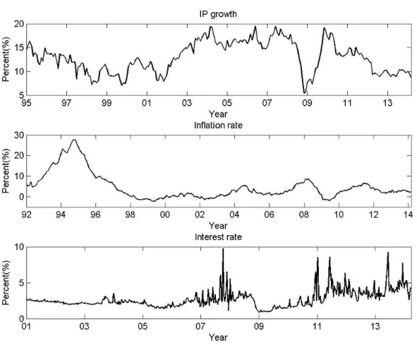
[Figure 1. Plot of the three macroeconomic variables]

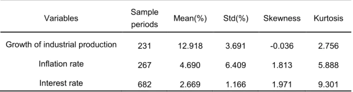
Table 1 presents the simple statistics for the three time series. All three time series exhibit high persistence that is easily visualized from the autocorrelation functions in Figure 2, where the autocorrelations slowly decay. This feature indicates that either the series possess relatively long memory or there are structural changes driving spurious persistence.

The interest-rate series presents clustering of volatility and jumps in the dynamics that imply changing volatility in innovation. This evidence provides the justification for our application of an adaptive approach that features a globally changing, locally stationary data-generating process.

[Table 1. Statistics of the three macroeconomic variables]

[Figure 2. Autocorrelation functions of the three variables]

3.2 LAR forecast procedure

Due to data availability, the three macroeconomic time series have different sample periods and frequencies. Thus for each time t estimation and its out-of-sample forecast, we set the maximum length of interval I_t^(K) to 120 +h periods for all variables (h denotes the forecast horizon). To reduce the computational burden when identifying the homogenous interval at timet, we use a universal set of sub-samples withK = 20 andM = 6 at each time point, starting with the shortest sub-sample covering the most recent six lag periods, setting the interval between two adjacent sub-samples to six periods, and ending with the longest sub-sample of 120 +h periods. Once an optimal sub-sample is selected against the next longer sub-sample, the parameter change is understood to have taken place sometime within the six periods in between. In doing so, we trade off precision in break identification for computational efficiency. Precise identification of the breaking point is not a major concern, however, since our primary goal is to estimate from the identified sample with relatively

(10)

homogeneous parameters. Also, as many changes occur smoothly, point identification of breaks need not be precise or even necessary.

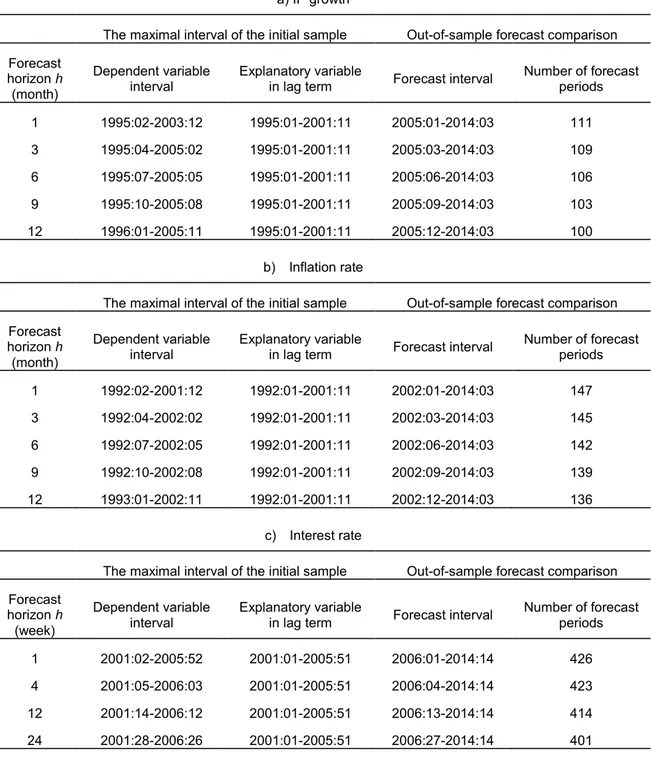
The resulting initial samples for a specific forecast horizon and the forecast comparison periods are summarized in Table 2. For monthly data of inflation and IP growth, we make out-of-sample 1-, 3-, 6-, 9- and 12-month ahead forecasts, and then move forward one month at a time to forecast at these five horizons until we reach the end of the full sample. For the weekly 7-day interbank offered rate, the first sample for estimation uses data up to end 2005 for 1-, 4-, 12-, and 24-week ahead forecasts. Then we move forward one week at a time to forecast at these four horizons until we reach the end of the full sample.

[Table 2. Initial samples of estimation and periods of forecast comparison]

3.3 Alternative models for comparison

For comparison, we choose popular forecast models for each macroeconomic variable. The choice of regression windows follow rule of thumb, either using a rolling window of 60 or 120 periods, or using a recursive window incorporating an increasing number of past observations as the forecast moves forward. A recursive window approach is preferred if the sample has no changing parameters and the extended sample length increases information efficiency. A rolling window approach addresses the balance of information efficiency versus possible breaks and resulting parameter uncertainty. In both cases, however, the choice of window length is predetermined and not selected in a systematic, data-driven manner.

Using the direct forecast approach as for the h-step ahead forecast of LAR(1) in equation (3), we also specify the alternative models forh-step ahead forecast as a generalized 1-step ahead forecast by lagging the predetermined dependent variablesh-step backward.

In addition to model comparison, we also use the CMRC Langrun survey forecast as an alternative. The predictive power of the Langrun survey forecast is reputed to be unbeatable as it combines the outlooks of forecast institutions in possession of rich information and using sophisticated forecast methods. The Langrun survey was initiated in July 2005 by the China Center for Economic Research (CCER) of Peking University. After the official release of the previous quarter’s data, the CMRC invites about two dozen institutions to predict the major macroeconomic variables for the next quarter, including GDP growth, CPI, industrial production growth, interest rates and exchange rates. The resulting CMRC Langrun forecast provides two measures: a simple average of institutional forecasts and a weighted average based on the historical forecast accuracy of each participating institution.

We assess how our LAR(1) model performs compared to the alternative models with various predetermined window length strategies and the Langrun forecast. We denote IP

(11)

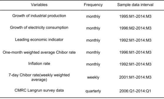
growth, CPI inflation rate and the 7-day Chibor at timetasy_t,π_tandr_t, respectively. The involved data in the alternative models, as will be mentioned in the following, are summarized in Table 3. Due to data availability, the intervals of data varies. This occasionally binds our choices of alternative window length selection in forecast comparison.

[Table 3. Summary of involved data in alternative models]

3.3.1 Alternative forecasts for IP growth

1. Time-series model of AR(1). Using a direct forecast approach as in the h-step ahead forecast of LAR(1) in equation (3), the AR(1) model for h-step ahead IP growth forecast is

yt=θ₀+θ₁yt−h+εt, εt∼N(0, σ_t²), (4) and its corresponding time-tforecast is

yb_t+h/t=θb₀+θb₁y_t. (5)

2. Real-activity-related model (RA). AsShiu and Lam(2004);Chen et al.(2007);Narayan et al.(2008) note, there is a strong correlation between real economic growth and real activity variables such as electricity consumption. In such models, in addition to lagged industrial production, a variable correlated with the real economy, X_t, is included,

yt=θ0+θ1yt−h+θ2Xt−h+εt, εt∼N(0, σ²_t). (6) We choose two alternatives forXt, either the electricity consumption or a leading economic indicator constructed by National Bureau of Statistics of China, both retrieved from the CEIC database. We denote these two versions of RA models as RA1 and RA2.

3. Interest-rate term-structure model (TS). Based on the RA model, the nominal risk- free rate, represented by the one-month weighted average national interbank offered rate of the People’s Bank of China, rt, is included. This short-term interest rate is an important monetary policy instrument. It is closely linked to the business cycle and carries useful information for forecasting performance of the real economy in the short to medium run. While it would be useful to consider the term spread (the difference between long-term and short-term interest rates) as it may be more effective in predicting business cycles, we limit our term-structure information to the short rate.

(12)

China has only had an active treasury bond market producing a meaningful yield curve since 2006. The TS model is thus written as

yt=θ0+θ1yt−h+θ2Xt−h+θ3rt−h+εt, εt∼N(0, σ²_t). (7) Here, the TS model with electricity consumption growth as additional related real activityXt−h is denoted as TS1, with the leading indicator as Xt−h denoted as TS2, and with both variables in Xt−h denoted as TS3.

4. Random walk (RW) model.

yt=yt−h+εt, εt∼N(0, σ_t²). (8)

yˆ_t+h/t = ˆyt. (9)

5. Langrun survey forecast.

The CMRC Langrun survey forecast is a quarterly forecast at the annual frequency for year-on-year growth rate that dates from the third quarter of 2005. Our IP growth data, in contrast, are for monthly year-on-year growth rates. Thus we transform our monthly results for 3-, 6-, 9-, and 12-months ahead forecasts into quarterly year-on- year growth data corresponding to 1-, 2-, 3-, and 4-quarter ahead forecasts with the following equation (10) (Mariano and Murasawa,2003):

y_t= 1

3 y_t−2^∗ +y^∗_t−1+y_t^∗, (10) wherey_tdenotes the transformed quarterly data, andy_t^∗ represents the corresponding monthly data.

For the same underlying realizationyt,we compare the 1- to 4-quarter ahead LAR(1) forecasts (ˆy_t|t−h,h= 1, ...,4) with (quasi) 1-quarter ahead Langrun forecasts (ˆy_t|t−1).

3.3.2 Alternative forecasts for the inflation rate

1. Time-series model AR(1).

πt=θ0+θ1πt−h+εt, εt∼N(0, σ²_t), (11) and its corresponding forecast is

πb_t+h/t=θb0+θb1πt. (12)

(13)

2. Phillips curve model (PC).

In addition to the lagged inflation, a variable proxying real activity, X_t, is also included:

π_t=θ₀+θ₁πt−h+θ₂Xt−h+ε_t, ε_t∼N(0, σ²_t), (13) where we choose two alternatives forX_t, either the IP growth or the leading economic indicator constructed by the National Bureau of Statistics of China. We denote these two versions as PC1 and PC2, respectively.

3. Interest-rate term-structure model (TS).

Based on the PC model, the nominal risk-free rate, represented by the one-month Chibor,rt−h, is included to provide potential information closely linked to the business cycle.

π_t=θ₀+θ₁πt−h+θ₂Xt−h+θ₃rt−h+ε_t, ε_t∼N(0, σ_t²). (14) The TS model with IP growth as Xt−h is here denoted as TS1, with the leading indicator asXt−h denoted as TS2, and with both IP growth and the leading indicator asXt−h denoted as TS3.

4. Random walk model (RW).

πt=πt−h+εt, εt∼N(0, σ²_t). (15)

ˆπ_t+h/t = ˆπ_t. (16)

5. Langrun survey forecast.

As with the IP growth forecast, the CMRC Langrun survey forecast for inflation is also a quarterly forecast for year-on-year inflation from the third quarter of 2005 onwards, while our CPI inflation is a monthly year-on-year inflation rate. We thus transform our monthly forecasting results for 3-, 6-, 9-, and 12-month horizons into quarterly year-on-year growth data corresponding to 1-, 2-, 3-, and 4-quarter horizons with the following equation (17)(Mariano and Murasawa,2003):

πt= 1

3 π_t−2^∗ +π_t−1^∗ +π_t^∗, (17) where πt denotes the transformed quarterly inflation data, and π^∗_t represents the corresponding monthly inflation data.

For the same underlying realizationπ_t,we compare the 1- to 4-quarter horizon LAR(1) forecasts (ˆπt|t−h,h= 1, ...,4) with (quasi) 1-quarter horizon Langrun forecasts (ˆπt|t−1).

(14)

3.3.3 Alternative models for key interest rate

1. Time-series model AR(1).

r_t=θ₀+θ₁rt−h+ε_t, ε_t∼N(0, σ²_t), (18) and its corresponding forecast is

rb_t+h/t=θ^b0+θ^b1rt (19)

2. Random walk (RW) model.

rt=rt−h+εt, εt∼N(0, σ²_t). (20)

rˆ_t+h/t = ˆrt. (21)

3.4 Measures of forecast comparison

We use three measures as indicators of forecast precision, the forecast root mean squared error (RMSE), the mean absolute error (MAE) and the mean error (ME). We also com- pute the standard deviation of absolute errors (Std(AE)) and standard deviation of errors (Std(Err)) to evaluate the forecast variation.

• Root mean squared error, RMSE.

RM SE = v u u t

1 Ti

Ti

X

t=1

(x_t−x_b_t)². (22)

• Mean absolute error, MAE, and standard deviation of absolute errors, Std(AE).

M AE = 1 Ti

Ti

X

t=1

|x_t−x_bt|, (23) Std(AE) = std(|x_t−x_b_t|), (24) whereTi is the forecasting interval, x_bt is the estimator for time t.

• Mean error, ME, and standard deviation of errors, Std(Err).

M E = 1

T_i

Ti

X

t=1

(xt−x_bt), (25)

Std(Err) = std(xt−x_bt). (26)

(15)

4 Forecast results

This section discusses comparison of forecasts, the potential monitoring function of the LAR approach on identifying shifts occurring as part of the economic transition, as well as robustness with respect to the forecast period.

4.1 LAR model performance compared to alternative forecasts

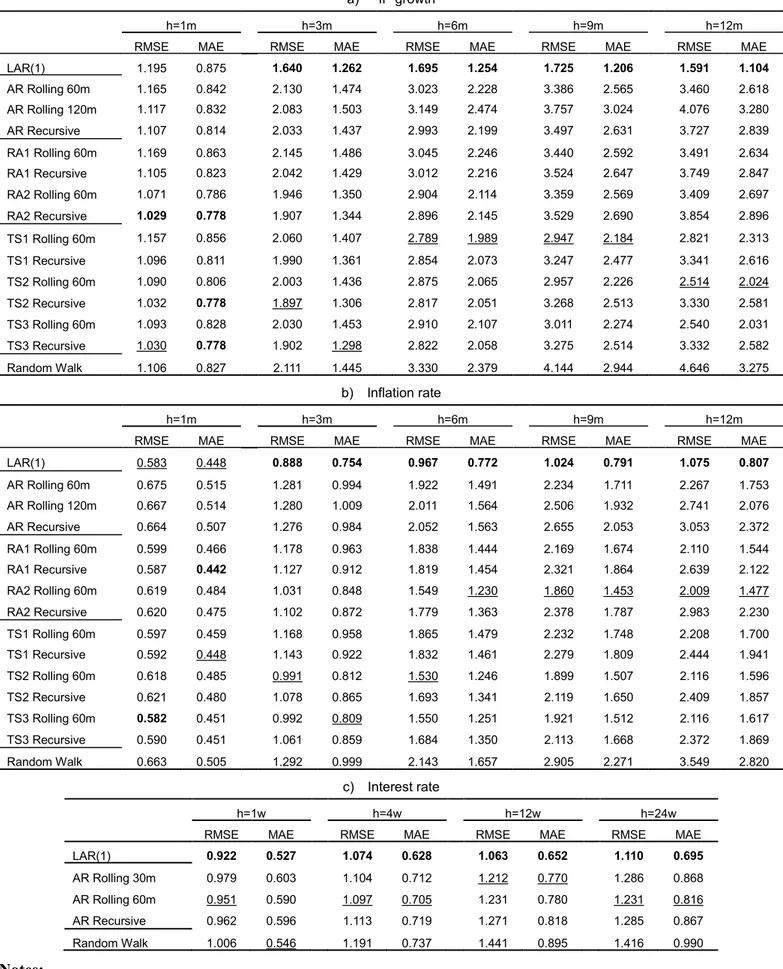
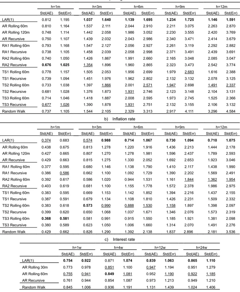
Table 4 reports the forecast RMSE and MAE, while Table 5 reports Std(AE) and Std(Err) for the macroeconomic variables with the selected forecast horizons.

For IP growth and the inflation rate, we compare the out-of-sample forecast performance for the LAR(1) model and the following alternative models and sample selection strategies:

(1) The autoregressive time-series model with three window-length strategies: 60- and 120-month rolling windows of fixed sample lengths, as well as a recursive window with expanding sample length.

(2) Other models with additional macroeconomic variables, including the real activity model (RA1, RA2) for IP growth and Phillips curve model (PC1, PC2) for inflation rate (both incorporating electricity or a leading indicator), and models incorporating the interest rate term structure (TS1, TS2, TS3) for IP growth and inflation. These models all have two alternative sample length strategies: a 60-month rolling window with fixed length and a recursive window with expanding sample length.

(3) The random walk model.

For the weekly interest rate Chibor, we presents the results of LAR(1), AR(1) with 130-week (2.5 year) and 260-week (5-year) rolling windows and a recursive window with expanding length, and the random walk.

In each column, the best forecast is indicated in bold across the forecast measure/horizon.

The second-best forecast is underlined.

[Table 4. Forecast comparison of the three macroeconomic variables: RMSE and MAE]

[Table 5. Forecast comparison of the three macroeconomic variables: Std(AE) and Std(Err)]

Table 4 demonstrates that the LAR(1) model for the three macroeconomic variables always outperforms alternative models in 3- to 12-month ahead forecasts. Moreover, the advantage increases with the length of the forecast horizon. With respect to IP growth and inflation, the RMSE and the MAE for 6- to 12-month ahead forecasts with the LAR model achieve a nearly 40–50 % reduction compared to the second-best forecast. The superior

(16)

performance of the LAR model over the alternatives is similar for the interest-rate forecast measured by RMSE and MAE, where both are the smallest for LAR in each forecast horizon.

Table 5 shows the LAR model outperforming the alternatives in 3- to 12-month ahead forecasts when forecast variance is considered in terms of standard deviation of mean absolute error and mean error. For IP growth, the reduction of standard errors tends to range between 10–40 % as the forecast horizon increases from 3 months to 12 months. A similar pattern is found for the inflation-rate forecast.

Overall, the LAR model outperforms alternative models except at the very short end (1-week and 1-month ahead forecasts). The superior performance of 3- to 12-month ahead forecasts for IP growth and inflation rate, as well as 4- to 24-week ahead forecasts for the interest rate, are robust with respect to measures of RMSE, MAE and standard deviations of forecast errors.

In Figure 3, we plot forecast comparison between the LAR and TS2 recursive forecast for IP growth, TS3 rolling 60m forecast for inflation rate, and AR 60m rolling forecast for interest rate. The first two rows present the forecast of IP growth and inflation rate for 1-, 6-, 9- and 12-month ahead forecasts, and the last row for 1-, 4-, 12- and 24-week ahead interest-rate forecasts. The realized data are displayed with solid lines, LAR forecasts are displayed with dashed lines, while the alternative forecasts have dot-dashed lines.

Because they are so close, it can be difficult to distinguish between the three series for the 1-period ahead forecast. Nevertheless, as the forecast horizon increases, it is clear that the dashed line of the LAR forecast tracks the dynamics of actual data more closely than the alternatives. In particular, the LAR 6-month, 9-month and 12-month ahead forecasts promptly capture sharp falls in IP growth and the inflation rate for the large swings during the financial crisis in the period 2007–2010.

[Figure 3. Plots of the realized data with forecasts of LAR and representative comparing models]

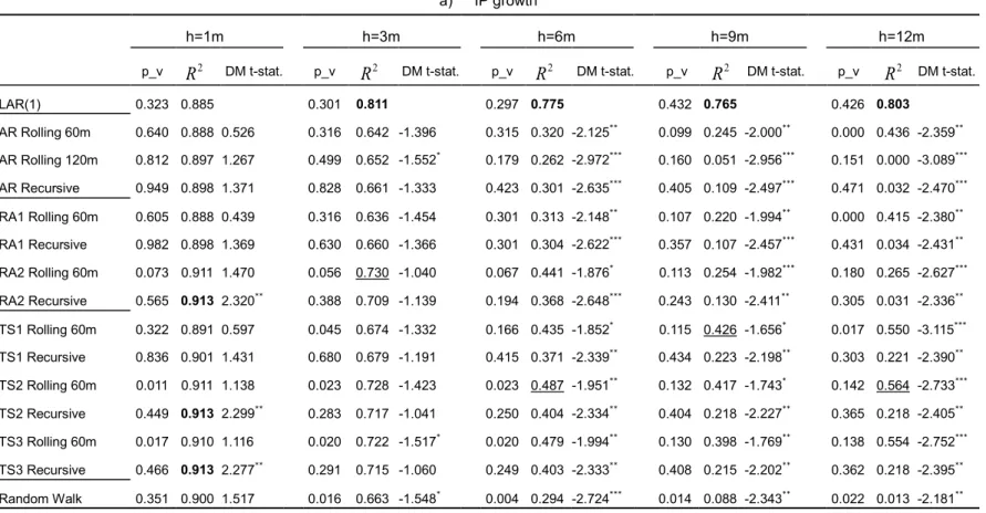
In Table 6, we report theR² in the Mincer-Zarnowitz regressions (Mincer and Zarnowitz, 1969) and the Diebold-Mariano test statistics (Diebold and Mariano, 1995) to compare the LAR versus alternative model forecasts. In the Mincer-Zarnowitz (MZ) regression, we regress the observed actual data on the corresponding forecasts of modeli:

y_t=α+βyˆ_t,i+ε_t, (27)

and take the determination coefficient R² as an indicator of forecast fit. Bold numbers indicate the highest R², the best forecast fit among the LAR and all alternatives. In the

(17)

Diebold-Mariano (DM) test, we conduct a pairwise test on the equality of the mean squared forecast errors by regressing the difference between the squared forecast errors of the LAR model and the alternative model i, e²_t,LAR−e²_t,i = µ+ε_t. The null hypothesis of equal performance is that H₀ :µ = 0. We focus on the t-statistics of parameter µ, denoted as DM t-stat, which favors the LAR if it is significantly negative (significance level marked by asterisks).

Table 6 shows that although the advantage of the LAR is insignificant for the 1-month ahead forecast for IP growth and inflation. However, it outperforms all alternative models in the 3- to 12-month ahead forecasts with the largest R² and significantly negative DM test statistics. Similar patterns hold for the interest-rate forecast across horizons.

[Table 6. Forecast comparison between the LAR and alternative models: MZ regression and DM test]

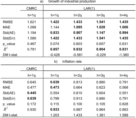
In Table 7, we compare the forecast performance of the LAR model against the CMRC Langrun survey: IP growth in panel a), and inflation rate in panel b). For comparison with the quarterly survey forecast, we transform our 3-, 6-, 9- and 12-month ahead forecast data into 1-, 2-, 3- and 4-quarter ahead year-on-year forecast data with equation (10) and (17). To match the same forecast period of inflation and IP growth, and in view of the incompleteness of the involved forecast institutes at the initial stage of CMRC survey, we discard the first two forecasts of the CMRC survey and conduct forecast comparison for both variables over the period 2006:Q1–2014:Q1. The CMRC column presents the 1-quarter ahead survey forecast. For the same targeted forecast period, we present 1- to 4-quarter ahead predictions of the LAR. We first report the measures of RMSE, MAE and standard deviations of errors. At the bottom of each panel, we provide two additional measures: the R² of MZ regression and the DM test statistics.

In panel a), the LAR outperforms the CMRC survey for IP growth on most measures, including smaller values for RMSE and standard deviation of errors and higherR²in the MZ regression in the case of the 1-quarter ahead prediction. Even in the 2-, 3- and 4-quarter ahead forecasts, the LAR model produces precision comparable to the 1-quarter horizon forecast and with higherR² in the MZ regressions and negative (even if not significant) DM t-statistics. In panel b), the performance of the LAR model matches that of the CMRC survey 1-quarter ahead inflation-rate forecast. The LAR model, however, produces overall satisfactory results compared to the survey forecast and delivers more timely prediction of forecast events than the CMRC survey.

[Table 7. Forecast Comparison between the LAR and CMRC survey]

(18)

In Figure 4, we plot the LAR and CMRC survey forecasts for the IP growth rate and inflation rate 1-quarter ahead in the first row. The actual data are indicated with solid lines, LAR forecast with dashed lines and survey forecast with dot-dashed lines. The figure shows that the LAR and CMRC survey forecasts match the actual data both very well, but the LAR better forecasts the economic downturn in 2008. The second row presents the actual data with solid lines, together with the LAR forecasts 2-, 3- and 4-quarter ahead marked as dashed lines, dotted lines and dot-dashed lines, respectively. Even for the 2- to 4-quarter ahead predictions, the LAR model captures the realized data without showing the dramatic rising prediction errors that typically accompany longer horizon forecasts.

[Figure 4. Plots of the realized data with LAR and CMRC forecasts]

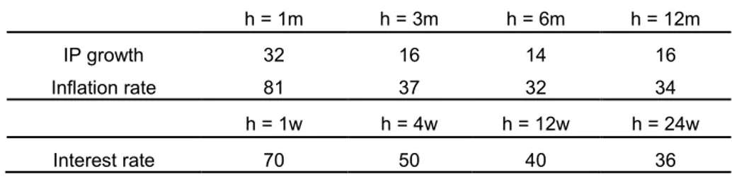
4.2 Lengths of stable sub-samples

Table 8 summarizes the average lengths for detected homogenous intervals of the three variables in each forecast horizon. The average sample length is relatively low with a mean value 19 months for IP growth. The average range of homogenous interval is 32–80 months for inflation and 36–70 weeks for interest rates. These average stable lengths are much shorter than the traditionally used sample lengths of, say, 5 years, 10 years or even longer in rolling and recursive window forecasts.

[Table 8. Average lengths of homogeneous intervals detected by LAR]

Figure 5 presents the parameter evolution in the LAR model for a 1-period ahead forecast with the three variables. We see here that the estimated parameters change over time with abrupt breaks and gradual changes that indicate regime shifts. The financial crisis dramatically drags down the persistence of inflation and interest rate, and pushes up standard deviations for all variables to historical highs.

[Figure 5. Parameter evolution in the LAR model]

4.3 Patterns of implied breaks and policy changes

Having shown our LAR model predicts selected Chinese macroeconomic variables better than traditional alternatives, we now consider if there might be other benefits from the model’s adaptive feature. Is useful information hidden in the detected breaks and parameter

(19)

shifts that drives good predictive ability of the model? Understanding the time-varying features of state dynamics in real time, after all, could be valuable not just for forecasting, but for real-time diagnosis of the macroeconomy and policy making.

Figure 6 plots the detected stable sub-samples and breaks along the vertical time axis for each macroeconomic variable. We report the results of the 1-step ahead forecast of the LAR(1) model. The vertical axis denotes the time when the forecast is made. At each point of time, an optimal sub-sample is detected. This is shown as a light solid line along the horizontal time axis. At the end of the line, a dark dotted line indicates the period, in this case six months for IP growth and inflation rate and six weeks for interest rate, during which the most recent break happens such that the hypothesis of homogenous interval no longer holds. When these (dark blue) dotted lines are stacked along the forecast time, common areas of detected breaks become evident.

[Figure 6. Detected sub-samples of homogeneity]

Observing Figure 6, we find that the stable sub-samples of the inflation rate are relatively longer than those of IP growth and interest rate as illustrated by the average sample lengths in Table 8. The real variable, IP growth, has fewer clear cut breaks with short homogeneous intervals, suggesting gradual and smooth changes in the data-generating process.

This finding echoes the gradual transition strategy of China and the diffusion of growth factors such as technology innovation, human capital development and the implementation of gradual institutional reforms. In contrast, the nominal variables for inflation rate and interest rate have several commonly identified ending periods of the homogeneous intervals, that is abrupt breaks in late 1994, early 2005 and early 2009 for inflation, and early 2004 and early 2008 for interest rates.

Nominal variables are prone to impacts of monetary policy and regime changes. Although break identification is purely data driven and a by-product of testing homogenous intervals for local estimation, commonly identified break periods in the nominal variables are quite in line with major policy changes. For instance, 1994 marks the official response to the economic overheating that began in 1992. At that time, the People’s Bank of China (PBoC) embraced monetary policies that have ever since kept inflation below 10 %.

Over our common samples of interest rate and inflation between 2001 to 2014, the LAR identifies two break periods for each variable. The breaks for interest rate (early 2004 and early 2008) leads the breaks for inflation (early 2005 and early 2009) by about a year. This is consistent with the stickiness of price and sensitivity of interest rate to policy changes.

However, what policy changes might have caused such substantial dynamic changes in the nominal variables?

(20)

First, there was the launch of marketization of interest rates in China in January 1, 2004.

The PBoC allowed commercial bank lending rates to float between 0.9 to 2 times the official lending rate. As a result, interest-rate formation became partly determined by the market and bank interest rates began to vary in response to supply and demand. There were also preparations for a change in exchange rate regime from a fixed to managed float in July 2005. A period of stable inflation ended as inflationary pressure began to build in mid-2005 in anticipation of yuan appreciation and large inflows of international capital.

Second, there was an abrupt change in monetary policy stance in the first half of 2008. At that time. the PBoC increased bank reserve requirements four times, eventually reaching 16.5%, the highest level since 1985. The reserve ratio averaged about 10% between 1985 and 2007. This tightened monetary policy ended some of the overheating in credit markets and altered interest-rate dynamics. However, with global financial crisis depressing Chinese exports and economic growth, the drop in inflationary pressure turned into a deflation nightmare in 2009, and ending another period of stable inflation.

Overall, our LAR method is useful in monitoring structural breaks of the economic process, showing gradual and smooth transition in the real economic variable, and abrupt changes in nominal variables which are largely in line with major monetary policy shifts.

4.4 Stability and robustness of the LAR forecast performance

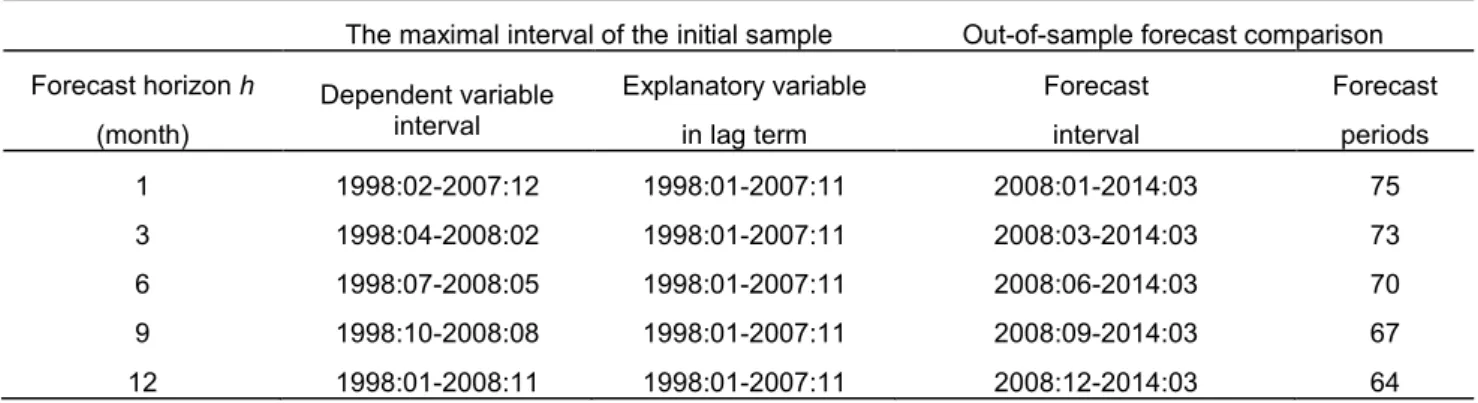
The LAR model demonstrates outstanding forecast performance for the three key macroeconomic variables. Is the performance restricted to the above-specified sample periods? The extreme large swings before 1997 may favor the LAR due to its quick detection and shedding off the initial period for the later forecast. Thus, the LAR may enjoy specific advantage in forecasting the IP growth and inflation rate compared to rolling window or recursive forecast of alternative models. To test the stability and robustness of the LAR forecast performance, we select the period of 1998:1 to 2007:12 as the initial sample to estimate and forecast the period of 2008:1 to 2014:3, a period that includes the global financial crisis.

We use similar procedures to those described above, including the same set of alternative models and similar forecast comparison measures.

The results are summarized in Table 9. Panel a) reports the concrete estimation time spans and forecast intervals for each forecast horizon. Panels b) and c) provide the forecast comparison in terms of RMSE, MAE and standard deviations of errors. In each column, the first best is bolded and the second best underlined. Results in panel b) and c) yet again show that the LAR outperforms alternative models for 3- to 12-month ahead forecasts for both IP growth and inflation. The reduction in RMSE, MAE and standard deviations of errors remains in the range of 10–50 % with respect to the second-best model. Again, the advantage increases with the forecast horizon. Panel d) provides the comparison with

(21)

MZ regression and DM test, where the advantage of LAR begins to dominate alternative models starting from 3-month ahead forecast horizons with significant p-values, the highest R-square and significant negative DM statistics. This robustness check demonstrates that the advantage of the LAR in 3- to 12-month ahead forecasts of real activity and inflation is maintained across sample periods.

[Table 9. Robustness check with sub-sample forecast for IP growth and inflation rate]

5 Conclusion

This study demonstrates how a LAR model may be applied to forecasting three key macroeconomic variables for China in a way that captures the features of its transition economy.

Our proposed method is shown to outperform popular models and window selection methods in predicting real and nominal out-of-sample variables, as well as display remarkable real-time monitoring power in detecting structural changes in the underlying economy. An ability to make timely, precise predictions can serve market participants and policymakers in assessing and monitoring economic dynamics.

Extension of the proposed LAR to forecasting other economic variables should be fairly straightforward. Future studies could also extend application of a LAR with exogenous variables (LARX) to improve forecasts and model-averaging based on an adaptive method.

(22)

References

Ahumada HA, Garegnani ML. 2012. Forecasting a monetary aggregate under instability:

Argentina after 2001. International Journal of Forecasting 28: 412–427.

Ang A, Bekaert G, Wei M. 2007. Do macro variables, asset markets, or surveys forecast inflation better? Journal of Monetary Economics 54: 1163–1212.

Bai J, Ng S. 2002. Determining the number of factors in approximate factor models.Econo- metrica 70: 191–221.

Bai J, Ng S. 2008. Forecasting economic time series using targeted predictors. Journal of Econometrics 146: 304–317.

Banerjee A, Marcellino M, Masten I. 2008. Forecasting macroeconomic variables using diffusion indexes in short samples with structural change, volume 3. Emerald Group Publishing Limited.

Belmonte M, Koop G. 2014. Model Switching and Model Averaging in Time-Varying Pa- rameter Regression Models. Bayesian Model Comparison 34: 45–69.

Bräuning F, Koopman SJ. 2013. Forecasting macroeconomic variables using collapsed dynamic factor analysis. International Journal of Forecasting .

Castle JL, Clements MP, Hendry DF. 2013. Forecasting by factors, by variables, by both or neither? Journal of Econometrics 177: 305–319.

Chen ST, Kuo HI, Chen CC. 2007. The relationship between GDP and electricity consumption in 10 Asian countries. Energy Policy 35: 2611–2621.

Chen Y, Härdle WK, Pigorsch U. 2010. Localized realized volatility modeling. Journal of the American Statistical Association 105: 1376–1393.

Chen Y, Niu L. 2014. Adaptive dynamic Nelson–Siegel term structure model with applications. Journal of Econometrics 180: 98–115.

Chow GC. 2015. China’s Economic Transformation. Wiley-Blackwell, third edition.

Clark TE, McCracken MW. 2010. Averaging forecasts from VARs with uncertain instabilities. Journal of Applied Econometrics 25: 5–29.

Clements MP, Hendry DF. 1996. Intercept Corrections and Structural Change. Journal of Applied Econometrics 11: 475–494.

(23)

Clements MP, Hendry DF. 2008. Economic forecasting in a changing world. Capitalism and Society 3.

D’Agostino A, Gambetti L, Giannone D. 2013. Macroeconomic forecasting and structural change. Journal of Applied Econometrics 28: 82–101.

De Gooijer JG, Hyndman RJ. 2006. 25 years of time series forecasting. International Journal of Forecasting 22: 443–473.

Diebold FX, Mariano RS. 1995. Comparing predictive accuracy. Journal of Business and Economic Statistics 20: 253–263.

Forni M, Hallin M, Lippi M, Reichlin L. 2000. The generalized dynamic-factor model:

identification and estimation. Review of Economics and Statistics 82: 540–554.

Forni M, Hallin M, Lippi M, Reichlin L. 2003. Do financial variables help forecasting inflation and real activity in the EURO area? Journal of Monetary Economics 50: 1243–1255.

Geweke J, Jiang Y. 2011. Inference and prediction in a multiple-structural-break model.

Journal of Econometrics 163: 172–185.

Härdle WK, Hautsch N, Mihoci A. 2014a. Local adaptive multiplicative error models for high-frequency forecasts. Journal of Applied Econometrics .

Härdle WK, Mihoci A, Ting CHA. 2014b. Adaptive order flow forecasting with multiplicative error models. Technical report, Sonderforschungsbereich 649, Humboldt University, Berlin, Germany.

Krkoska L, Teksoz U. 2007. Accuracy of GDP growth forecasts for transition countries:

Ten years of forecasting assessed. International Journal of Forecasting 23: 29–45.

Lin JY. 2013. Demystifying the Chinese Economy. Australian Economic Review 46: 259–

268.

Mariano RS, Murasawa Y. 2003. A new coincident index of business cycles based on monthly and quarterly series. Journal of Applied Econometrics 18: 427–443.

Mincer JA, Zarnowitz V. 1969. The evaluation of economic forecasts. InEconomic Forecasts and Expectations: Analysis of Forecasting Behavior and Performance. NBER, 1–46.

Narayan PK, Narayan S, Prasad A. 2008. A structural VAR analysis of electricity consumption and real GDP: evidence from the G7 countries. Energy Policy 36: 2765–2769.

Naughton B. 2007. The Chinese economy: transitions and growth. MIT press.

(24)

Rossi B, Sekhposyan T. 2010. Have economic models’ forecasting performance for US output growth and inflation changed over time, and when? International Journal of Forecasting 26: 808–835.

Shiu A, Lam PL. 2004. Electricity consumption and economic growth in China. Energy policy 32: 47–54.

Stock J, Watson M. 2009. Forecasting in dynamic factor models subject to structural instability. The Methodology and Practice of Econometrics. A Festschrift in Honour of David F. Hendry : 173–205.

Stock JH, Watson MW. 1999. Forecasting inflation. Journal of Monetary Economics 44:

293–335.

Stock JH, Watson MW. 2002a. Forecasting using principal components from a large number of predictors. Journal of the American Statistical Association 97: 1167–1179.

Stock JH, Watson MW. 2002b. Macroeconomic forecasting using diffusion indexes. Journal of Business and Economic Statistics 20: 147–162.

Stock JH, Watson MW. 2007. Why has US inflation become harder to forecast? Journal of Money, Credit and Banking 39: 3–33.

Stock JH, Watson MW. 2008. Phillips curve inflation forecasts. Technical report, National Bureau of Economic Research.

(25)

Table 1. Statistics of the three macroeconomic variables

Variables Sample

periods Mean(%) Std(%) Skewness Kurtosis Growth of industrial production 231 12.918 3.691 -0.036 2.756

Inflation rate 267 4.690 6.409 1.813 5.888

Interest rate 682 2.669 1.166 1.971 9.301

Notes:

The first row is monthly data of the growth rate of industrial production from 1995:1 to 2014:3; the second row is the monthly CPI inflation rate from 1992:1 to 2014:3; the third row is the selected interest rate, the weekly 7-day Chibor (China Interbank Offered Rate), taken from the weighted average closing rate of the last trading day of a week, from January 2001 to March 2014. All data are from CEIC China Economic and Industry Database.

(26)

Table 2. Initial samples of estimation and periods of forecast comparison

a) IP growth

The maximal interval of the initial sample Out-of-sample forecast comparison Forecast

horizon h (month)

Dependent variable

interval Explanatory variable

in lag term Forecast interval Number of forecast periods

1 1995:02-2003:12 1995:01-2001:11 2005:01-2014:03 111

3 1995:04-2005:02 1995:01-2001:11 2005:03-2014:03 109

6 1995:07-2005:05 1995:01-2001:11 2005:06-2014:03 106

9 1995:10-2005:08 1995:01-2001:11 2005:09-2014:03 103

12 1996:01-2005:11 1995:01-2001:11 2005:12-2014:03 100

b) Inflation rate

horizon h (month)

Dependent variable

1 1992:02-2001:12 1992:01-2001:11 2002:01-2014:03 147

3 1992:04-2002:02 1992:01-2001:11 2002:03-2014:03 145

6 1992:07-2002:05 1992:01-2001:11 2002:06-2014:03 142

9 1992:10-2002:08 1992:01-2001:11 2002:09-2014:03 139

12 1993:01-2002:11 1992:01-2001:11 2002:12-2014:03 136

c) Interest rate

horizon h (week)

Dependent variable

1 2001:02-2005:52 2001:01-2005:51 2006:01-2014:14 426

4 2001:05-2006:03 2001:01-2005:51 2006:04-2014:14 423

12 2001:14-2006:12 2001:01-2005:51 2006:13-2014:14 414

24 2001:28-2006:26 2001:01-2005:51 2006:27-2014:14 401

(27)

Table 3. Summary of involved data in alternative models

Variables Frequency Sample data interval

Growth of industrial production monthly 1995:M1-2014:M3 Growth of electricity consumption monthly 1996:M2-2014:M3 Leading economic indicator monthly 1992:M1-2014:M3

One-month weighted average Chibor rate monthly 1996:M1-2014:M3

Inflation rate monthly 1992:M1-2014:M3

7-day Chibor rate(weekly weighted

average) weekly 2001:M1-2014:M3

CMRC Langrun survey data quarterly 2006:Q1-2014:Q1