Forecasting Swiss exports using Bayesian forecast reconciliation

Research Collection

Journal Article

Forecasting Swiss exports using Bayesian forecast reconciliation

Author(s):

Eckert, Florian; Hyndman, Rob J.; Panagiotelis, Anastasios Publication Date:

2021-06-01 Permanent Link:

https://doi.org/10.3929/ethz-b-000456815

Originally published in:

European Journal of Operational Research 291(2), http://doi.org/10.1016/j.ejor.2020.09.046

Rights / License:

Creative Commons Attribution-NonCommercial-NoDerivatives 4.0 International

This page was generated automatically upon download from the ETH Zurich Research Collection. For more information please consult the Terms of use.

ETH Library

ContentslistsavailableatScienceDirect

European Journal of Operational Research

journalhomepage:www.elsevier.com/locate/ejor

Production, Manufacturing, Transportation and Logistics

Forecasting Swiss exports using Bayesian forecast reconciliation ^R

Florian Eckert

^a,∗

, Rob J. Hyndman

^b

, Anastasios Panagiotelis

^c

aKOF Swiss Economic Institute, ETH Zurich, Leonhardstrasse 21, Zürich 8092, Switzerland

bDepartment of Econometrics and Business Statistics, Monash University

cDiscipline of Business Analytics, University of Sydney, Australia

a r t i c l e i n f o

Article history:

Received 9 April 2020 Accepted 28 September 2020 Available online 3 October 2020 Keywords:

Forecasting

Hierarchical reconciliation Optimal combination Decision-making

a b s t r a c t

Thispaperproposes anovelforecast reconciliationframework using Bayesian state-spacemethods. It allowsforthejoint reconciliationatallforecasthorizons andusespredictivedistributionsrather than pastvariation offorecast errors.Informative priors areusedto assignweights tospecific predictions, whichmakesitpossibletoreconcileforecastssuchthattheyaccommodatespecificjudgmentalpredic- tionsormanagerialdecisions.Thereconciledforecastsadheretohierarchicalconstraints,whichfacilitates communicationandsupportsaligneddecision-makingatalllevelsofcomplexhierarchicalstructures.An extensiveforecastingstudyisconductedonalargecollectionof13,118timeseriesthatmeasure Swiss merchandiseexports,groupedhierarchicallybyexportdestinationandproductcategory.Wefindstrong evidence thatin addition toproducing coherent forecasts, reconciliationalso leadsto substantial im- provementsinforecast accuracy.The useofstate-spacemethods isparticularly promisingfor optimal decision-makingunderconditionswithincreasedmodeluncertaintyanddatavolatility.

© 2020TheAuthors.PublishedbyElsevierB.V.

ThisisanopenaccessarticleundertheCCBY-NC-NDlicense (http://creativecommons.org/licenses/by-nc-nd/4.0/)

1. Introduction

Forecastsare essentialtothe decision-makingprocessinbusi- ness analytics and macroeconomics. At an aggregate level, they are often strategic and, therefore, subject to judgmental adjust- ments andmanagerialdecisions.Atmoredisaggregateoperational levels, forecasts usually rely onstatistical methods. Ifthe datais subject to linear hierarchical constraints, predictions generated from different methods and informationsets are usually not co- herent. Insome instances, incoherentpredictionsare problematic because they may lead to contradictory conclusions and non- aligned decision-making. Furthermore, incoherent forecasts are oftendifficulttocommunicate.Anexpostadjustmentofforecasts to ensure coherence resolves these issues and has been shown to lead to substantial improvements in forecast accuracy (see Wickramasuriya, Athanasopoulos, andHyndman, 2019,and refer- ences therein). This paper proposes a novel approach to jointly reconcile all forecastingperiodsusingBayesian state-spacemeth- ods.Itallowsfortheidentificationandshrinkageofcoherenceer- rors,whichmeansspecificpredictionscanbe assignedweights in

R Hyndman and Panagiotelis are grateful for support from the ARC Centre of Ex- cellence for Mathematical & Statistical Frontiers.

∗Corresponding author.

E-mail address: eckert@kof.ethz.ch (F. Eckert).

theprocessofreconciliation. Itmayoccur,forinstance,thatman- agerialdecisionsarereflectedinscenarioforecastsatthestrategic level,butnotinforecastsattheoperationallevel.Iftheprediction atthestrategiclevelisbelievedtobemoreaccurate,theproposed methodallowsthereconciliationofincoherentforecastssuchthat the entire hierarchy is consistent with the initial prediction for the strategic level. This supports aligned decision-making across alloperationalunitswhilemaintainingahighdegreeofflexibility.

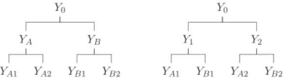
Hierarchicaldatacanbestructuredaccordingtovariouscharac- teristics such asgeographical,organizational,societal ortemporal features (Kourentzes& Athanasopoulos,2019). Swissmerchandise exports,forexample,canbedisaggregatedgeographicallyintodes- tinationregions, such asWestern Europe,North Americaor Aus- tralia. These regional aggregates can then be divided further by country.Totalexportscanalsobedisaggregatedintoproductcate- gories,suchasprecisioninstruments,textilesorvehiclesandthen further intosubcategories, such asroad, rail,air andwater vehi- cles.As aresult,thedatahasthestructureofaso-calledgrouped hierarchy(seeWickramasuriyaetal.,2019,andreferencestherein).

Fig.1givesasimpleexampleofgroupedstructurewithk=3lev- els,m=9seriesintotalandq=4seriesatthemostdisaggregate or‘bottom’level.

Since it is known that all future realizations of the data will adhereto the constraints implied by theaggregation structure, a desirableproperty ofanyforecastsis thatthey alsorespectthese

https://doi.org/10.1016/j.ejor.2020.09.046

0377-2217/© 2020 The Authors. Published by Elsevier B.V. This is an open access article under the CC BY-NC-ND license ( http://creativecommons.org/licenses/by-nc-nd/4.0/ )

Fig. 1. Simple Example of a Grouped Hierarchy . The data is structured into k = 3 levels, m = 9 time series in total and q = 4 time series at the bottom level.

constraints.Suchforecastsarereferredtoas‘coherent’.Earlierlit- erature reducedthe issueof producing coherentforecaststo one of predicting only a specific level of the hierarchy. For example, the‘bottom-up’approach(Gross&Sohl,1990)achievescoherence by producingonly forecasts forthe bottom-level series andthen summingtheseupaccordingtothehierarchicalstructure.Amajor shortcomingofthisapproachisthatdisaggregateseriestendtobe noisyandthereis ahighrisk ofmodelmisspecification. Features such asseasonalitymaybe impossibletoidentify inthebottom- level data, despite being clearly present in the aggregate series.

Toaddressthisshortcoming, a‘top-down’approachwasproposed (see Athanasopoulos,Ahmed,andHyndman,2009,andreferences therein), wherethepredictedtop levelseriesisdisaggregatedac- cording to historical or forecasted proportions of lower levels. A compromiseisgivenbythe‘middle-out’approach,wherethefore- casts atan intermediate levelofthehierarchyaresummed upto get thehigherlevelsanddisaggregatedtoobtain lower-levelpre- dictions.A weaknessofthesesingle-level methodsis information loss becausethetimeseriescharacteristicsatotherlevels arenot takenintoaccount.

In responseto theseshortcomings,therehas beena tendency over thepastdecadetowards producingforecastsforall seriesin thehierarchyratherthanonlyatasinglelevel.Thesearereferred toas‘base’forecastsandtheygenerallydonotadheretoaggrega- tion constraints.Forecast reconciliation, introduced by Hyndman, Ahmed, Athanasopoulos, and Shang (2011), performs an ex post adjustmenttobaseforecastsinordertoproduceanewsetofco- herent forecasts. Thisadjustmenteffectivelycombinespredictions fromalllevelsandindoingso‘hedges’againstmisspecificationer- ror acrosstheentirehierarchy.Ithasbeenshownrepeatedlythat linearcombinationsofpredictionmodelsleadto betterandmore robustforecasts(see,forinstance,Conflitti,Mol,&Giannone,2015;

Stock & Watson, 2006). There is now substantial theoretical and empiricalevidencethatforecastreconciliationcansignificantlyim- prove forecast accuracyforhierarchicaldata (seeWickramasuriya etal.,2019,andreferencestherein).

Inordertoencodetheaggregationconstraintsinahierarchy,y_t isdefinedtobeanm-vectorthatstacksobservationsattimetfrom allseries,b_t tobeasubvectorofy_t containingonlytheqbottom- level seriesattimet andSto bean m×qaggregation matrix.In thesimplegroupedhierarchyshowninFig.1,thesearegivenby

y_t (m×1)=

⎡

⎢ ⎢

⎢ ⎢

⎢ ⎢

⎢ ⎢

⎢ ⎣

Y0

Y_A YB

Y1

Y₂ YA1

YA2

Y_B1 YB2

⎤

⎥ ⎥

⎥ ⎥

⎥ ⎥

⎥ ⎥

⎥ ⎦

(mS×q)=

⎡

⎢ ⎢

⎢ ⎢

⎢ ⎢

⎢ ⎢

⎢ ⎣

1 1 1 1

1 1 0 0

0 0 1 1

1 0 1 0

0 1 0 1

1 0 0 0

0 1 0 0

0 0 1 0

0 0 0 1

⎤

⎥ ⎥

⎥ ⎥

⎥ ⎥

⎥ ⎥

⎥ ⎦

bt (q×1)=

⎡

⎢ ⎣

YA1

YA2

YB1

YB2

⎤

⎥ ⎦

^.

Here and in general, the matrix S is defined such that y_t= Sbt holds forall realized data. Toreconcile these base forecasts, Hyndmanetal.(2011)andlaterauthorsassumedthefollowingre- gressionstructure:

y_t

(

^h

)

=S

β

h+et

(

^h

)

, (1)

where y_t

(

^h

)

^{is an m-vector containing the h}-periods-ahead base forecastsattime tforeach levelinthehierarchy. Theerrorterm et

(

^h

)

^{hasmeanzeroandcovariancematrix}

h,and

β

hrepresents the unknown mean of the bottom-level series which combines informationaboutforecastsatalllevels.Itcanbe estimatedusing theregressionequation

β

h=

SW⁻_h¹S ⁻¹SW⁻_h¹y_t

(

^h

)

. (2)

A vector of reconciled forecasts is then given by S

β

h and will adhere to the aggregation constraints by construction. There are several potential choicesfor W_h. Letting W_h=Im corresponds to an ordinary leastsquares estimate, inthe following alsoreferred to asa ‘noscaling’ estimate. Alternatively, a highdegree of het- eroskedasticity in the error terms motivates a diagonal W_h or weightedleast squares approach (Hyndman, Lee, & Wang,2016).

Underso-called‘variancescaling’,weightsarethevariancesofin- sampleh-stepaheadforecastvariances,andforecastswithlessac- curate historical performance are down-played in reconciliation.

Another alternative is the ‘structural scaling’ approach suggested byAthanasopoulos,Hyndman,Kourentzes,andPetropoulos(2017), wherebyweightsarebasedonthenumberofseriesaggregatedat each node. Morerecently, the ‘MinT’approach wasdeveloped by Wickramasuriyaetal.(2019)to allowforaW_h thatisnot diago- nalandexploits thecovariancesbetweentheh-step-aheadrecon- ciledforecast errors.Thenomenclaturereferstothefact thatthis approachminimizesthetraceofthecovariancematrixofreconcil- iationerrors. Thesemethods reconcile each forecast period inde- pendentlyandsometimesuseascaledversionofW₁foreachhto simplifycomputations.

This paper contributes to the literature on forecast reconcil- iation and aligned decision-making in various ways. First, it in- troducesan explicitidentificationofthe reconciliationerrorsand provides arepresentationin state-spaceform. Thisallows forthe jointreconciliationofallforecast horizonsforcrosssectionaland grouped hierarchies, thereby extending the established literature (see, forexample, Wickramasuriyaet al., 2019) whereeach hori- zon isreconciled independently andthe reconciliationbiases are treatedaspartoftheerrorterm. Second, incontrastto thevari- ance scaling (Athanasopouloset al., 2017) orMinT approach, the weights used in the reconciliation are derived from the predic- tivedistributionratherthanpastvariationofthebaseforecaster- rors.Ourinnovation is, therefore,particularlypromising forfore- castingmodelsthatallowforconditionalheteroskedasticity.Third, we introduce an efficient Bayesian estimation algorithm that en- ables the inclusion of prior information. We exploit informative priors to shrink the influence of particular series irrespective of past forecasting performance. This is valuable ifforecasters have strong judgmental reasons for believing that a particular model willworkwellinthefuturewhileotherbaseforecastswillbeless reliable.Theproposed framework,therefore,alsoexploresweight- ing options thatmay not necessarilyincrease predictive accuracy butcanbeveryusefulinoperationalforecasting.Theuseofinfor- mative prior distributions also allows the occurrenceof negative reconciled forecastsand singularforecast errorcovariance matri- ces tobe addressed. Whilethe recentworkof Corani,Azzimonti, andZaffalon(2019)andBenTaiebandKoo(2019)respectivelytake aBayesianapproachandemployshrinkageinreconciliation,these considerationsarenottakenintoaccountintheirframeworksand they donotreconcileall forecast horizonsjointly.Lastly,thepro- posed model and existing methods are evaluated using a com- prehensive grouped hierarchy of Swiss merchandise trade. Apart from the comparative analysis, this application provides insights forpublicauthoritiesaswellasexportingfirms.Merchandisefore- castsoftenserveasinputsintoprojectionsofotherquantitiessuch assales,inventories,currencyreservesandproductioncapacity.

The remainder of the paper is structured as follows.

Section 2introduces ournovelBayesian state-spacereconciliation framework andan efficientestimationalgorithm. Section3 intro- ducesindetailthedataon exportsofSwissgoods,usingmodern techniques for exploring and visualizing high-dimensional time series. Section 4 conducts an extensive forecast evaluation that compares ourproposed methodwithexisting reconciliationtech- niques. In addition, it highlights the usefulnessof bias shrinkage forapplicationsinoperationalforecasting.Section5concludes.

2. ReconciliationusingBayesianstate-spacemethods

This section proposes a novel approach to forecast reconcilia- tion. Weshow how toexplicitly identifythereconciliationerrors andestimatethemaslatentstatesthatevolveovertheforecasting horizon. Our method involves the use of predictive distributions instead ofhistorical forecast errorsanduses prior informationto addressseveralissuesintheliterature.

2.1. Model

An integrated reconciliation of all forecasted periods has the advantage of combining information across the entire forecast- ing horizon. If a base forecast in any given forecasted period is revised downwards as a result of the reconciliation, it is likely to be revised downwards as well in the next period. This de- pendency can be taken into account using state-space methods, which could further improve forecasting accuracy. Pennings and van Dalen (2017) pioneered their use in order to integrate the reconciliationofincoherentinformationacrosstime periods.They assume the bottom-level series to be the underlying states and use elaborate state equations to capture their stochastic proper- ties. While thistakes the intertemporal dependencies nicelyinto account,itrequirestheestimationofinitialstatesandrestrictsthe number ofusablemodels for thebase forecasts. We proposethe explicit identification ofstate-dependent reconciliationerrors

α

h, which leaves the coherent bottom-level forecasts

β

h completely freeofanyassumptionsorrestrictions:

E[y_T+h]=S

β

h=E[y_T

(

^h

)

^]−

α

h (3) The expected h-step-ahead reconciled forecastsare givenby S

β

h. Them-dimensionalvector

α

h=E[y_T

(

^h

)

^]−S

β

hcontainstherecon- ciliationbiases.Itcanbeinterpretedasafixedeffectthatisunique toeachforecastedvariable.Sisasummationmatrixoforderm×q andtheq-vector

β

hestimatestheunknownmeanofthereconciled bottom-level forecasts. The measurement equation is then given as

yT

(

^h

)

=

α

h+S

β

h+eT

(

^h

)

, eT

(

^h

)

∼N

(

⁰,

h

)

. (4) The m-vector e_T(h) consists of h-step ahead base forecast er- rors that follow a normal distribution with mean zero and co- variance matrix

h. It can be estimated by taking a sample of n prediction errors eˆ_T

(

^h

)

^{from the predictive} distribution of y_T(h).Samplingfromthepredictivedistributionallowsalsotoob- tain an estimate for the mean of the incoherent base forecasts E[y_T

(

^h

)

^]=yˆ_T

(

^h

)

^{. These draws may originate fromposterior pre-} dictive distributions resulting from Bayesian forecasting models (Amisano&Geweke, 2017),bootstrapaggregating(Bergmeir,Hyn- dman,&Benítez,2016),modelpooling(Kapetanios,Mitchell,Price,

& Fawcett, 2015; Timmermann, 2006), or sampling froma fitted model(Hyndman&Athanasopoulos,2018).

Inordertoreconcileallforecastinghorizonsjointly,thecoher- ence errors

α

h are modeled to be state-dependent. They are as- sumed to follow a random walk, which is very common in the literature ontime-varyingparameters (see,forinstance,Primiceri, 2005,andreferencestherein).Thisimpliesthat thebestguessfor

acoherenceerrorinanygivenforecastingperiodistheerrorinthe precedingperiod.Thestateequationis,therefore,specifiedas

α

h=

α

h−1+v_h, v_h∼N

(

⁰,

)

. (5) The initialstate

α

0 isthe coherenceerror inthelast observation y_T,whichisconvenientlyknownto bezero.Itishoweverneces- sarytoimpose somerestrictions inordertoidentifytheparame- ters,whichisa resultofmulticollinearity inEq.(3).This isquite intuitivesincethereismorethanoneuniquewaytoreconcilein- coherentforecasts.Toshow thisformally,thecoherenceerrors

α

h

can be expressed equivalentlyby concentrating out

β

h using the projectionmatrixP_h=S

(

^S

⁻h¹S

)

^−1S

⁻h¹.Thisleadstothefollow- ing identity:

(

^Im−P_h

) α

h=

(

^Im−P_h

)

^yˆT

(

^h

)

. It is useful to define theidempotent residual makerM_h=Im−P_h.Since M_h isnot in- vertibleduetothepresenceofmulticollinearity,theidentity can- notbesolvedfor

α

h.Ouridentifyingassumptionisthat

α

h liesin thespanofM_h,inwhichcaseM

α

h=

α

h.Thissolvestheidentifi- cation problemandleavesthe reconciliationbiases asa function ofthedataandtheresidualmakerM_h.Thisresultisalsointuitive sincethe reconciliationbiasesare theresiduals fromaregression ofthebaseforecastsontheaggregationmatrix.¹

2.2. Estimation

The latent states are sampled jointly using the efficient state smoothing and simulation algorithm proposed by Chan and Jeli- azkov(2009).Wegetthemarginaldistributionsbyapproximating thejointposteriordistributionviaGibbssamplingfromthecondi- tionaldistributions(Ando&Zellner,2010).Convergenceisachieved veryquickly,irrespectiveofthestartingvalues.We takeasample ofsize 1000 fromthe joint posteriordistribution after a burn-in of100draws.ThemeasurementEq.(4)isstackedovertheHfore- castingperiodsinorderto reconcileallreconciliationerrorstates jointly.

y=X

α

+Z

β

+e, e∼N

(

⁰,

)

, (6) wheretheparametersofinterestaregivenby

((H+1

α

)m×1)=

⎡

⎣ α

⁰

..

α

.H

⎤

⎦

,

β

(Hq×1)=

⎡

⎣ β

1

..

β

.H

⎤

⎦

,

(^Hm

×Hm)=

⎡

⎣

^{1 .}..

H

⎤

⎦

.

Theunreconciledbase forecastmeans ˆyT

(

^h

)

,thesummation ma- tricesandsomefurtheridentitiesarestackedaccordinglyinto

(Hmy×1)=

⎡

⎣

ˆ y_T

(

¹

)

.. . ˆ y_T

(

^H

)

⎤

⎦

, X (^Hm×(^H+1)^m)=

⎡

⎣

Im

0 ... Im

⎤

⎦

,

(HmZ×Hq)=

⎡

⎣

S ...

S

⎤

⎦

.

ThestateEq.(5)needstobewrittencorrespondinglyas

F

α

=v, v∼N

(

⁰,Q

)

⁽⁷⁾

where

(^Hm×(F^H+1)^m)=

⎡

⎢ ⎢

⎣

Im

−Im Im

... ...

−Im Im

⎤

⎥ ⎥

⎦

^,

1See Appendix A.1 for a detailed derivation.

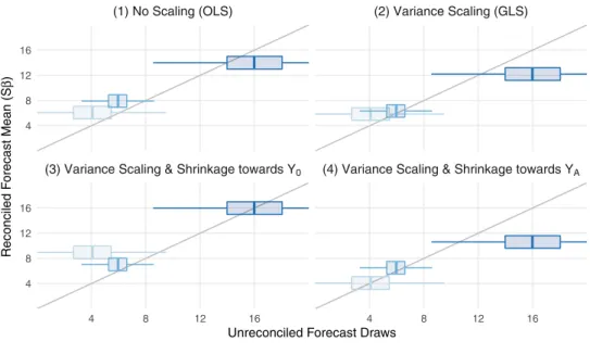
Fig. 2. Prior Weighting Schemes . The 45 ^◦line indicates where the unreconciled base forecasts on the x-axis are equal to reconciled forecast means on the ordinate.

(HmG×Hm)=

⎡

⎢ ⎢

⎣

0

...

⎤

⎥ ⎥

⎦

^.

Theinitialstate

α

0isknowntobezerosinceitcorrespondstothe coherenceerrorinthelastobservationy_T.Itissufficienttochoose

0 very small in order shrink the initial state

α

0 towards zero.

Furthermore,thestackedresidualmakercanthenbecalculatedas M=I_Hm−Z

(

^Z

^−1Z

)

^−1Z

^{−1.Usingthe}identificationdescribedin Section 2,it is then straightforward to rewrite the stacked mea- surementEq. (6)as

My=X

α

+e, e∼N

(

⁰,

)

. (8) FollowingChanandJeliazkov(2009),theconditionalposteriordis- tributionof

α

^{isthengivenby}

α

^∼N

(

^a1,A₁

)

^{where A}1=

(

^FG−1F+X

^−1X

)

⁻¹ a1=A1

(

^X

^−1My

)

.

This algorithm is computationally very efficient if block-banded matrices and sparse matrix algorithms are used. Following Chan and Jeliazkov (2009), it is even faster to compute the banded CholeskyfactorofA₁ andsolvefora₁ byforward-andbackward substitution.Thebottom-levelmeans

β

^{areretrievedfrom}

β

∼N

(

^b1,B1

)

^{where B}1=

Z

^−1Z+B⁻₀^{1 −1} b₁=B₁

Z

⁻¹

(

^y−X

α )

+B⁻₀¹b₀ . The priorsb₀ andB₀ should bechosen tobeasuninformativeas possible.Aninconvenienteffectofmostreconciliationmethodsis the occurrenceofnegativereconciled bottom-levelforecasts. This might be a concernsince manyapplications such assales orex- ports do not allow for negative observations. Using a truncated normalprior,thisissuecanberesolved inanuncomplicatedfash- ionby simplydiscardingdrawsof

β

^{thatcontain negativeentries}

duringthesamplingprocess.

The covariance matrix of the state equation errors

^{is cho-} sen to bediagonal because thereconciliationerrors are assumed tobe uniqueforeachbaseforecastmodel.Thediagonalelements

ω

1,...,

ω

mcanberetrievedfromaninverse-gammadistribution:

ω

i∼IG

(

^c1/2,d1/2

)

, where c1=c0+H

d1=d0+

( α

h,i−

α

h−1,i

)

( α

h,i−

α

h−1,i

)

where

α

h,idenotes thereconciliationerrorofseries i∈

{

¹,...,m

}

atforecastingperiodh∈

{

¹,...,H

}

^{.Wechoose aweaklyinforma-}

tiveproperpriordistributionwithc₀=3andd₀=0.01inorderto restrictthemovementofthereconciliationbiasesslightly.

Thecovariancematrixofthebaseforecasterrors

hisassumed tobediagonalaswellsinceitcanbeverycumbersometoestimate inlargehierarchiesandforlongerforecastinghorizons.The diag- onalelements

σ

1,h,...,

σ

m,hare,therefore,drawnfromaninverse- gammadistributionaccordingto

σ

i,h∼IG

(

^k1/2,l1/2

)

, where k1=k0+n

l1=l0+eˆi,T

(

^h

)

^eˆi,T

(

^h

)

.

The n-dimensional vector eˆ_i,T

(

^h

)

^{represents the ex-ante known} predictionerrors forvariable i∈

{

¹,...,m

}

, which havebeenob- tainedfromthepredictivedistributionofthebaseforecasts.While thisparsimoniousapproachhasadvantageswhenitcomestocom- putational speed and more accurate forecasts at lower levels of the hierarchy, it is possible to estimate the full covariance ma- trix of historical base forecast prediction errors in the spirit of Wickramasuriyaetal.(2019)orbyorderingthedrawsfromthein- dependentpredictivedistributionsfollowingJeon,Panagiotelis,and Petropoulos(2019).Bothapproacheswouldthen requiresampling fromaninverse-Wishart distributionandarelikely torequiread- ditionalshrinkagepriors.Forourparsimoniousapproachusingan inverse-gammadistribution,wechooseaweaklyinformativeprior distributionwithk₀=3 andl₀=1.Thishasnegligible impacton theposteriordistribution,butensuresthat

hisnonsingularinthe casewhereabaseforecasthasnovariation.

2.3. Biasshrinkage

Inordertoaligndecisionswithaspecificbaseforecast,itmay be of interest to selectivelyshrink some reconciliationbiases to- wardszero.Thisisespeciallyusefulwhenthereexistssome prior

knowledgethataparticularbaseforecastcontainsadditionalinfor- mation thatisnot reflectedinother levelsofthehierarchy.Since thecovariancematrixofthepredictionerrorsentersthemodelas aweightingmatrix,itcanbeusefultoimposepriorrestrictionson

h.Thiscanbeachievedusingatime-invariantdiagonalmatrix

withmweights onitsdiagonal.Fortheconjugateinverse-gamma prior describedin Section2.2,this impliesaparameter choice of k₀=nand l₀=

(

^eˆi,T

(

^h

)

^eˆi,T

(

^h

)) λ

i, where

λ

i is the weight of the ithvariableaccordingtothecorrespondingentryin

^.Thiscanbe interpretedasanempiricalBayespriorbecauseitisdefinedusing the knownbaseforecast errors.In ordertoshrink thereconcilia- tionbiastowardszero,thecorrespondingweight

^hastobeless thanone.Atthesametime,itisnecessarytoincreasetheremain- ingelementsaboveonesuchthattheyareabletoaccountforthe higher reconciliationbiasesattheir levelofthe hierarchy.Thisis achievedbyconstructingtheweightssuchthattheproductofthe diagonalelementsof

^{remains constantatunity.Asaresult,the} determinantandthereforethegeneralizedvarianceof

h

^re- mainsthesameforeach

^{(Mustonen,1997).}

Fig. 2 demonstrates the impact ofdifferent prior assumptions on theestimatedreconciliationbiases.It featuresidenticalunrec- onciled forecastsof a simple hierarchy with m=3 series, where Y_A+Y_B=Y₀. Foreach series a sampleis drawn from the predic- tive forecastsdensity, assumed to be N

(

⁴,2

)

^{for Y}A,N

(

⁶,1

)

^for Y_B,andN

(

¹⁶,3

)

^forY0.Thehorizontalaxisshowsdrawsfromthe unreconciledbaseforecasts,whichareclearlyincoherent.Thever- tical axis,onthe other hand, showsthemeans of thereconciled forecasts.Thediagonallineshowsvalueswherethemeansofbase and reconciled forecastsare equal. Forboxes above thisdiagonal line,reconciliationadjustsforecastsupwards.Forboxesbelowthe diagonalline,forecastsareadjusteddownwards.

Eachpanelcorrespondstoadifferentpriorchoicefor

h.Sub- figure (1) shows that the forecast biases for each margin are treated equally in an ordinary least squares regression, conse- quently the means ofY_A andY_B are adjusted upwards whilethe mean ofY₀ isadjusted downwards.Subfigure(2)showsreconcil- iation biases that are weighted with the inverse of their corre- spondingforecast variances.Thisleadstoa smalleradjustmentin YB (the reconciled andbase means are close) relative the others since it is more accurate. Subfigures (3) and (4) shrink the rec- onciled forecastsofY₀ andY_A towards theirbaseforecasts. There mayexistpriorinformationonthereliabilityofcertainmodelsor therequirementtofixsomeforecastsatspecificvalues.Thiscould be dueto betterdataavailability,highersuitabilityofaparticular modelorsubjectivejudgmentoftheforecaster.

Besides the shrinkage ofspecific reconciliation biasestowards zero, there are several other weighting methods conceivable.

Section4.4providesempiricalapplicationsandhighlightstheuse- fulnessofshrinkagereconciliationinoperationalforecasting.

3. Data

We use a comprehensive dataset containing exports of Swiss goods, collectedbytheSwissFederal CustomsAdministration.All timeseriescoveraperiodfrom1988to2018inmonthlyfrequency and are denominated in Swiss francs. They are not adjusted for seasonalitiesorcalendareffectsanddatarevisionsareusuallyvery insignificant. The data can be groupedby export destination and product category. The geographichierarchy consists of8 regions, aggregated from 245 countries and dependent territories. The categorical hierarchy follows a national nomenclature covering 12 main economic groups and 48 subgroups. This leads to a grouped hierarchywithm=13,118seriescontainingatleastone nonzero entryofwhich q=9,483 seriesare atthebottom level.

Table 1 provides summary statistics on the series at each level.

Furthervisualizationsonthechangeincompositionandadetailed

statementofallcategoricalandgeographicalclassificationscanbe foundinAppendixA.3.

All values shown refer to the invoiced price of the goods in Swiss francs, including transport and insurance costs as well as other expenditure up to the Swiss border. If the invoice is in a foreign currency, the invoiced amounts are converted using the previous day’sexchange rate. As aresult, the figures are affected by exchange rate fluctuations. However, prices respondin a way thatmitigatestheinfluenceofexchangeratefluctuations,duetoa quickexchangeratepass-through,documentedbyBonadio,Fischer, andSauré (2020)forimportsaswellasexports.

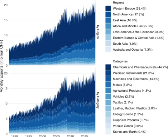
Fig.3showsthehistoricaldevelopmentoftheregionalandcat- egoricalhierarchies.Asaresultofitsstatusasasmallopenecon- omy ina rapidlyglobalizing world,Swiss exports haveincreased significantlysincethelate1980s.Accountingformorethanhalfof totalexports,WesternEuropeisakeymarketforSwissgoods.In- creasinglylarger shares of exports alsogo to North Americaand East Asia, with around 17% each in 2018. Exports to Africa and the Middle East, Latin America and the Caribbean, Central Asia andEasternEurope,SouthAsia,AustraliaandOceaniaaccountonly forabout10%combined.Thehierarchicalgroupingbycategoriesis moreevenly distributed,buthas beensubjecttogreater shiftsin itscomposition.Themostimportantcategoriesare‘Chemicalsand Pharmaceuticals’, ‘PrecisionInstruments’ and‘Machines andElec- tronics’.Thetwohierarchicalgroupingsarequitedifferent.Thege- ographichierarchywidenstowardsthebottom,butwithamajor- ityoftheexport volumegoing toEuropean countriesitis never- thelesshighlyconcentrated.Thecategoricalhierarchy,ontheother hand,hasfewersubgroupsandthereforeremains narrowtowards thebottom.Comparedtotheregionalhierarchy,theexportvolume ishowevermoreevenlydistributed.

Acommonassumptionisthat seriesatthetoplevelofahier- archyareeasiertoforecast.Duetotheaggregationinvolved,they areusually lessnoisyandexhibitmorepredictable characteristics suchasthestrengthofseasonality,trend,spectralentropy,andse- rial correlation.Kang, Hyndman,andSmith-Miles(2017) measure thisbyextractinganumberoftime seriesfeaturesfromthedata thatarecommonlyassociatedwithbetterpredictability.Theythen constructameasureofpredictabilityforeach timeseriesbyesti- matingprincipalcomponents fromthesefeatures. Figure4shows the first principal component, which accounts for a large share ofthe variation inthese predictabilityfeatures. It isevident that thereexistsastrongcorrelationbetweenpredictabilityandexport volume.

4. Reconciliationofexportforecasts

This section provides empirical evidence for the benefits of forecast reconciliation. It compares the performance of different reconciliation methods and explores which data characteristics profitinparticularfromhierarchicalcombination.Thesetupofour comprehensivepseudo-realtimeforecastingexerciseisdescribedin thefollowing.

A large hierarchy of Swiss goods exports is used to test the Bayesian reconciliation framework and various competing meth- ods. Ineach month from1995to 2015, forecastsfor all seriesin the hierarchyare calculated forthe next 36 months. Foreach of the13,118series,weuseafewunivariatebenchmarkmodelstoget thebase forecasts. It shouldbe noted thatthis isnot necessarily the bestmodel choice since we donot take intoaccount impor- tant explanatory variables such as exchange rates, relative prices or global economic developments. Our focus is to show the ad- vantagesofreconciliationforforecastingaccuracy,whichwedoby comparing reconciled predictions to unreconciled base forecasts.

Therefore,themethodusedto createthebaseforecastis notour primary consideration.We use an autoregressive integratedmov-

Table 1

Summary statistics for hierarchical levels.

Levels No. of Series Mean Std. Dev. Min Max IQR

Geographical Categorical

World Total 1 12,129 – - – –

World Category 12 1011 1340 66 4292 1023

World Subcategory 48 253 619 0 3844 137

Region Total 8 1516 2493 136 7498 1384

Region Category 96 126 344 0 2571 60

Region Subcategory 377 32 146 0 2271 9

Country Total 245 50 212 0 2527 14

Country Category 2848 4 29 0 683 0

Country Subcategory 9483 1 13 0 567 0

Notes: Summary statistics refer to the average monthly export volume in million Swiss francs of each series between 1988 and 2018.

Fig. 3. Contribution to Swiss Merchandise Exports of Goods . Monthly Swiss merchandise exports, denominated in billion Swiss francs, not adjusted for seasonalities or calendar effects. Average export shares of the year 2018 in parentheses.

ing averagemodel(ARIMA),an exponentialsmoothingstate-space model (ETS), and a seasonal random walk model (RW). As de- scribed in Hyndman and Khandakar (2008), the model for each series is parameterized automatically based on the Akaike Infor- mationCriterion.Inordertogetsamplesfromthepredictiveden- sities,n=1000samplepathsaresimulatedfromeachfittedmodel using Gaussian errors. With the exception of the volatile period during the Great Recession,the ARIMA and ETSapproaches out- performtherandomwalkonaverageforseriesateveryleveland forecasting horizon. All results in the following subsection will, therefore,relyonARIMAforecasts.²

Theseincoherentforecastsarethenreconciledusingseveralba- sicsingle-levelandoptimalcombinationmethods.Thesingle-level techniques include bottom-up, top-down and middle-out meth- ods. Thelattertwocanonly beusedfornon-groupedtime series

2A detailed description of the methodology and comparisons of forecasting methods, horizons and accuracy measures can be found in Appendix A.2 .

and are, therefore,tested on the regional and categorical hierar- chiesseparately.Thecombinationmethodsusedareordinaryleast squares (no scaling), weighted least squares with variance scal- ing, weighted least sqared with structural scaling, MinT and the Bayesianstate-spacereconciliationframework(BSR).Ifaggregation ofthepredictionerrorsisnecessary,they areweightedwiththeir respective export share. The reconciled forecasts are then com- paredtothecorrespondingunreconciledpredictionsusinglogrela- tiverootmeansquaredforecasterrors(Hyndman&Koehler,2006).

4.1. Comparisonofreconciliationmethods

Fig.5showstheaccuracyofallforecasts, definedasthelogof therootmeansquaredforecastingerrorofthe baseforecastsrel- ative to the mean squared errors of the coherent forecastsfrom eachmethod.Valuesabove zeroindicate,therefore,a betterfore- cast performance. It is worth noting that reconciliation meth- ods andbottom-up forecasts are the only techniques that allow

Fig. 4. Predictability of Different Levels in a Hierarchy . Predictability is defined as the first principal component of a large number of time series features described in Kang et al. (2017) .

Fig. 5. Relative Accuracy of Reconciliation Methods . Values above zero indicate higher forecast accuracy relative to the unreconciled case. Forecast accuracy is given by the log of the root mean squared forecast errors of the unreconciled forecasts relative to the reconciled forecasts. Average of all forecast dates and horizons.

for coherence across all levels ofa groupedhierarchy. Top-down and middle-out reconciliations are not applicable in the case of groupedtimeseries.

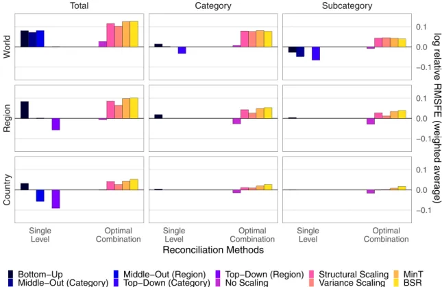
Fig.6 showsthat some forecastsdo notbenefitfromreconcil- iation. Especially for the bottom-level series, combination meth- ods appear to decrease forecastingperformance. Variance scaling and BSR are less affected by this deterioration of forecast accu- racy at lower levels, probably as a result of their parsimonious parameter choice. Inorder todemonstrate thebenefits ofhierar- chical combination, Fig. 6 shows average log relative RMSFEs by

weighting the prediction errors at intermediate and lower levels usingthecorrespondingshareintotalexportvolume.Itisevident that single-level methodsdo notconsistently improveforecasting accuracy.Thebottom-up andmiddleout methodsfarereasonably well forthe top level series,butfail to outperform the unrecon- ciledforecastsatlowerlevelsandaresometimesevensignificantly worse. Optimal combination,on theother hand, tendsto outper- form the baseforecasts especially for top and intermediate-level series.Especiallyvariance scaling,MinT andBSR workwell at all levels.

Fig. 6. Average Relative Accuracy of Reconciliation Methods . Values above zero indicate higher forecast accuracy relative to the unreconciled case. Forecast accuracy is given by the log of the root mean squared forecast errors of the unreconciled forecasts relative to the reconciled forecasts. Errors at intermediate and lower levels are weighted using their corresponding share in total export volume. Average of all forecast dates and horizons.

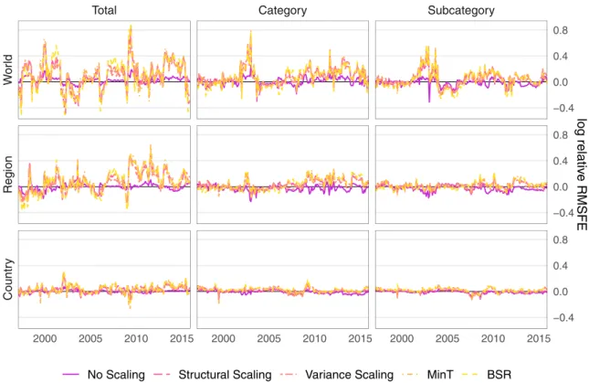
It isalsoinstructivetolookatthedevelopmentoftherelative forecasting accuracyover time in Fig.7. Eventhough thecombi- nation methods are moreaccurate on average, they do not con- sistently outperform theunreconciledforecasts. Whilethecombi- nationusingnoscalingdoesnotbeattheunreconciledbenchmark, theremainingmethodsperformbetterandfairlysimilarovertime.

Forthetoplevelseries,thebenefitsofreconciliationaccruemostly duringtimesofglobaleconomicdistressandcorrespondingappre- ciations of the Swiss franc.This is dueto the fact that the sim- plermodelsatlowerlevelsprovidestabilityattimeswhenthetop level model is biased. The biggest gains can be observed during theearly2000srecessionfollowingtheburstofthedot-combub- ble,theglobalfinancialcrisisandthefollowingsovereigndebtcri- sisinEurope,andthesuddenappreciationoftheSwissfrancafter the Swiss NationalBank stopped supporting the currency pegto theEuroinearly2015.Interestingistheforecastingaccuracyafter January2002,whenelectricalenergywasreclassifiedasagoodin- steadofaservice. Thestructuralbreakinthetimeseriesleadsto misspecifiedmodels,buttherigidstructureimposedbythehierar- chyincreasesforecastaccuracysubstantiallyrelativetotheunrec- onciledcase.

4.2. Comparisonofforecastinghorizons

Inordertocheck whetherthe accuracyimprovementsaresig- nificant, we test for equalityof the mean squared errors of rec- onciled and unreconciled forecasts. Since it is not possible to get unreconciledforecastsby constrainingtheparameter spaceof the reconciliationprocedure, thecomparison involvesnon-nested models. FollowingClark andMcCracken (2013),we thereforerely on theteststatisticproposed byDieboldandMariano(1995),us- ing the variance correction suggestedby Harvey, Leybourne, and Newbold (1997). It accounts for serialcorrelation in the squared errorloss whiletestingforsignificanceinthedifference between

twosquaredforecasterrorsatvariousforecastinghorizons.Table2 showsthe p-values for the one-sided test, where the alternative hypothesisisthattheaccuracyofreconciliationmethodsisgreater.

Withthe exception of themiddle-out approaches, single-level methodsarenotsignificantlymoreaccuratethantheunreconciled forecastsatallhorizons.Optimalcombinationsareassociatedwith lowerp-values,inparticularfortheperiodofincreasedeconomic volatility after the Great Recession. Parsimonious approaches, in particular no scaling or variance scaling, appearto perform best evenatlongerforecastinghorizons.Thereishowevernoevidence thattheuseofpredictivedistributionsandstate-dependentrecon- ciliationerrorsleadstosignificantgains.

4.3. Comparisonofhierarchicallevels

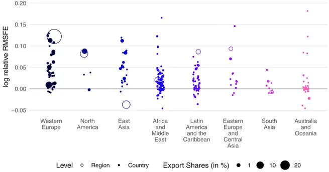
Anotherwaytodissecttheresultsistoidentifywhichtimese- riessee thegreatestgains inforecast accuracyfromusingrecon- ciliation. Fig. 8 provides an overview of the relative forecast ac- curacy bygeographicclassification, usingthe Bayesianreconcilia- tionframework.Itisagainobviousthatreconciledforecastsareon average more accurate than in the unreconciled case, but not in everyinstance.It appearsthatserieswithalarger exportvolume benefitmostfromreconciliation.Forecastsofexportstocountries inEurope,North AmericaandEastAsia arealmostentirelybetter off thaninthe unreconciledcase, whereasforecastsofexports to countrieswithalowershare,suchastheislands inOceania,tend tobeworseoff.Inaddition,atop-leveltimeseriesdoesnotneces- sarilybenefitmorefromreconciliationthanatimeseriesatlower levels.Thesameresultsalsoholdtruefortherelativeforecastac- curacybycategories,asshowninFig.9.Becausetheexportshares inthe categoricalhierarchyare more evenlydistributed, thepat- ternofsmallerexportvolumesbeingworse off duetoreconcilia- tionislesspronounced.Resultsforothervariancescalingmethods suchasweightedleastsquaresandMinTaresimilar.

Fig. 7. Relative Accuracy of Combination Methods over Time . Values above zero indicate higher forecast accuracy relative to the unreconciled case. Forecast accuracy is given by the log of the root mean squared forecast errors of the unreconciled forecasts relative to the reconciled forecasts. Errors at intermediate and lower levels are weighted using their corresponding share in total export volume. Average of all forecast horizons.

Table 2

Tests for predictive accuracy.

Entire Sample Moderate Period Crisis and Recovery

1998–2018 1998–2006 2007–2018

12 24 36 12 24 36 12 24 36

Single-Level

Bottom Up 0.49 0.28 0.29 0.84 0.86 0.67 0.10 0.12 0.14

Middle Out (Category) 0.14 0.05 ^∗ 0.17 0.28 0.13 0.09 0.19 0.16 0.33 Middle Out (Region) 0.02 ^∗ 0.04 ^∗ 0.01 ^∗ 0.08 0.15 0.05 0.08 0.10 0.02 ^∗ Top Down (Category) 0.11 0.14 0.13 0.16 0.15 0.14 0.16 0.14 0.08 Top Down (Region) 0.14 0.14 0.84 0.07 0.15 0.16 0.14 0.12 0.92 Optimal Combination

No Scaling 0.00 ^∗∗ 0.00 ^∗∗ 0.01 ^∗ 0.05 0.08 0.03 ^∗ 0.01 ^∗ 0.01 ^∗∗ 0.02 ^∗ Structural Scaling 0.05 ^∗ 0.04 ^∗ 0.09 0.37 0.40 0.19 0.00 ^∗∗ 0.02 ^∗ 0.06 Variance Scaling 0.02 ^∗ 0.01 ^∗ 0.05 ^∗ 0.22 0.15 0.07 0.00 ^∗∗ 0.01 ^∗∗ 0.05 ^∗ MinT 0.03 ^∗ 0.01 ^∗∗ 0.08 0.14 0.10 0.13 0.04 ^∗ 0.03 ^∗ 0.11

BSR 0.14 0.08 0.12 0.57 0.62 0.25 0.01 ^∗∗ 0.04 ^∗ 0.09

Notes: Table shows p -values of one-sided Diebold Mariano tests. They are retrieved by testing differences be- tween reconciled and unreconciled forecast errors, using the top level series and forecasting horizons of 12, 24 and 36 months. Significance indicated by ^∗∗∗p < 0.001, ^∗∗p < 0.01 and ^∗p < 0.05.

4.4. Benefitsforaligneddecision-making

Reconciliation techniques are useful for complex operational structures becausebaseforecastscan begeneratedindependently atallhierarchicallevels.However,itisusuallycostlytoincorporate specificadjustmentsintoallbaseforecastsastheyrelyondifferent methodsandinformationsets.Forinstance,somepredictionsmay contain managerialdecisions that aredifficult toincorporateinto models at other levels of the hierarchy. Because reconciliation procedures minimize the distance between coherent and inco- herent forecasts, it oftenoccurs that thejudgmental adjustments to a specific forecast are diluted because they are not reflected in other base forecasts. The reconciled forecasts allow then for aligned decision-making, but do not fully reflect the judgmental

adjustmentsto afew specific baseforecasts. Anadvantage ofthe generalized weighting scheme proposed in Section 2.3 is that the reconciliationerrors can be targeteddirectly. This allows the forecastertoshrinkcertainreconciledforecaststowardstheirbase forecast.

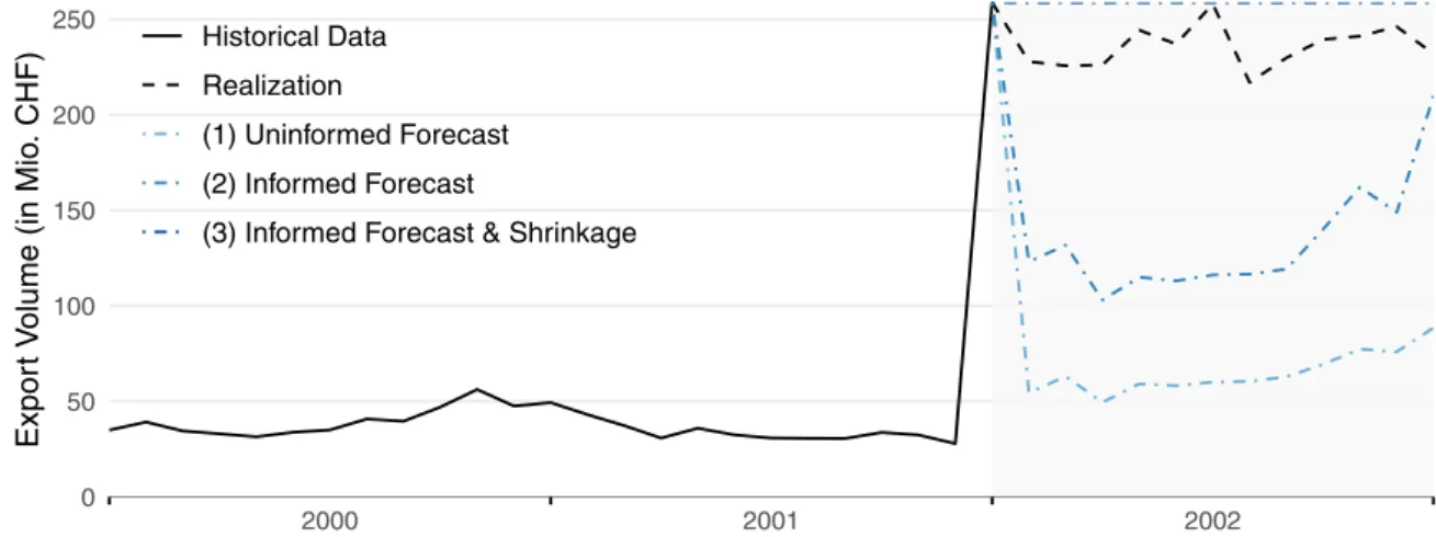
An example for the usefulness of shrinkage reconciliation is given by the reclassification of electricity as a good instead of a service in foreign trade statistics (see also Section 4.1). Starting in early 2002,this change inaccounting standardsincreased the share of energysources fromalmost 0% to more than 2% of to- talmerchandiseexports.Fig.10showsvariousforecastingscenar- ios forexports of energy sources. All predictions are based on a trainingsamplethatincludes historicaldata upthe firstobserva- tionwiththenewaccountingstandard.

Fig. 8. Relative Accuracy of Reconciliation Methods by Regions. Values above zero indicate higher forecast accuracy relative to the unreconciled case. Forecast accuracy is given by the log of the root mean squared forecast errors of the unreconciled forecasts relative to the reconciled forecasts. Average of all forecast dates and horizons.

Reconciliation using unweighted Bayesian state-space reconciliation.

Fig. 9. Relative Accuracy of Reconciliation Methods by Categories. Values above zero indicate higher forecast accuracy relative to the unreconciled case. Forecast accuracy is given by the log of the root mean squared forecast errors of the unreconciled forecasts relative to the reconciled forecasts. Average of all forecast dates and horizons.

Reconciliation using unweighted Bayesian state-space reconciliation.

Scenario (1) shows theforecast forexports ofenergy sources usingthesamemodelasbeforethestructuralchange.Itisevident thatitfailstocapturethestructuralbreakandadjustsveryslowly asmoreobservations pourin.Scenario(2) assumesajudgmental decisiontousearandomwalkforecastafterobservingtheincrease inexportvolumesinJanuary.Eventhoughtheforecasterhasprior knowledge thatarandomwalkforecast isappropriate forthisse- ries,the modelsatotherlevels assumethestructuralbreaktobe an outlier.Theydominateanyinformationfromtherandomwalk forecastanditisshifteddownwardsduringthereconciliationpro- cedure.Theonlysolutionwouldbeanadjustmentofthebasefore- castsforall otherseries,whichiscumbersomegiventhecomplex

categoricalandgeographicaldatastructure.Scenario(3)reliesona randomwalkforecastaswell, butusesshrinkagereconciliationto putmoreweightonthisparticularforecast.Thisforcestherecon- ciledpredictiontostayclosetoitsbaseforecast,whichprovidesa reasonableprojectionforexportsofenergysourcesin2002.

Sincethereconciliationproceduredistributesthecoherencyer- rorsacross the entirehierarchy, thisalso leadsto some accuracy gainsatotherlevels.Moreimportantly,itallowsmanagerstoalign their decisionswithother unitswithout sacrificingforecast accu- racy.Shrinkagereconciliationthusimprovesalignmentofdecisions across complex hierarchies by allocating more weight to predic- tionsinwhichmanagershavemoreconfidence.

Fig. 10. Forecasting Scenarios for Exports of Energy Sources. Monthly exports of energy sources from 20 0 0 to 20 02 in million Swiss francs. The structural break in January 2002 is caused by the reclassification of electrical energy as a good instead of a service.

Table 3

Deviations from base forecasts.

Target Level Evaluation Level Appropriate Methods Benchmark

Top-Down Bottom-Up Shrinkage

Top Level Total/World 0 0 0.6

Total/Region 37.2 2.4 1.0

Category/World 17.4 2.8 1.1

Category/Region – 3.0 11.6

Bottom Level Total/World 2.5 2.5 0.6

Total/Region 2.8 2.8 1.0

Category/World 3.6 3.6 1.1

Category/Region 0 0 11.6

Notes: Deviations from the base forecast are measured using mean absolute percentage errors. Predictions are gener- ated from ARIMA forecasts with a horizon of 12 months for each month from 1998 to 2018. Results from state-space reconciliation without shrinkage serve as benchmark.

Besides the shrinkage ofspecific reconciliation biasestowards zero,severalotherweightingmethodsareconceivable.Possibleap- proachesincludetheweightingofeachseriesbyitslevelinthehi- erarchyorbythe numberofseriesateachnode inthehierarchy.

This allows forthe emulation of the ‘structural scaling’,‘bottom- up’, ‘middle-out’ and ‘top-down’ approaches. This is particularly relevant for judgmental adjustments of forecastsin complex op- erationalstructures.Animportantexampleisthecasewherefore- castsatthetoplevelareassumedtobecorrectbecausetheycon- tain information on managerialdecisions that is not available to forecastersatlowerunits.Asaresult,allremainingbaseforecasts should bereconciled such thatthey arecoherentwiththeaggre- gateforecastatthestrategiclevel.Anothercommonexampleisthe casewhereforecastsatthemostdisaggregate,operationallevelare trustedmoreandpredictionsareaggregatedfromthebottomlevel.

Weillustratethesetwocasesbyreconcilingasetofpredictions usingtheappropriatesingle-level methods,namelytop-down and bottom-up reconciliation, and the Bayesian shrinkage approach.

Table3showsthedeviationsfromthebaseforecastsinmeanab- solute percentageerrorsforeachofthethreemethods.Deviations betweenbaseforecastsandstate-spacereconciliationswithoutany shrinkageserveascomparison.

Table 3 highlights a key contribution of the proposed frame- work, namelythat it can gearthe reconciledpredictions towards anydesiredbaseforecast.Itreplicatesallresultsfromthe‘bottom- up’ approach, which is intuitive given that the upper levels are aggregated from the bottom-level base forecasts. The shrinkage approach extends the scope of the ‘middle-out’ and ‘top-down’

methods because they cannot be used for grouped hierarchies.

Table3alsoshowsthatlowerreconciliationbiasesforsome fore-

casts comes at the cost of reconciled predictions being further awayfromtheirbaseforecastsatotherlevels.

5. Conclusion

Thispaperextendstheliterature onhierarchicalforecastcom- bination and aligned decision-making by introducing an explicit definitionofstate-dependentreconciliationbiases. Thisallowsfor the joint reconciliation of all forecast periods and combines in- formation on the coherence errors across the entire forecasting horizon. Furthermore, the Bayesian framework allows for the in- corporationofpriorinformationontheparameters,whichenables theforecastertointroducesubjectivejudgmentintothereconcili- ation.Inaddition,informativepriorsavoidsomeissuessuchasthe occurrence of negative reconciled forecasts and singularforecast errorcovariance matrices. The useof predictive densities instead of past forecast errors allows forgreater flexibility in the choice ofthe baseforecast models, taking, forinstance,conditional het- eroskedasticity intoaccount when weighting the forecastsatdif- ferent horizons. However, the approach tends to be slower than establishedreconciliationtechniquesbecauseitrequiressimulation ofthejointposteriordistributionusingGibbssampling.

Usinga comprehensivehierarchicaldatasetofSwissgoodsex- ports,wedemonstratethatoptimalcombinationmethodsimprove the forecasting accuracy significantly compared to the unrecon- ciledcaseandsimplerreconciliationmethods.Whilethe‘MinT’ap- proachshowsthelargestimprovements ataggregatelevels, more parsimonious approaches such as variance scaling or Bayesian state-space reconciliationimprovethe accuracyalso atmore dis- aggregatelevels.Eventhoughreconciledforecastsaresignificantly

more accurate on average, no reconciliation method consistently outperforms the unreconciled forecasts across the hierarchy or overtime.Forecastsataggregate levelstendtobenefitmorefrom reconciliationthannoisyseriesatthebottomofahierarchy.Atthe samelevel,forecaststhataccountforalargershareofthetotalare onaveragemoreaccurateafterreconciliation.Optimalcombination methods are shownto be particularlyuseful inthe case ofmis- specified modelsandduringperiodsofhighvolatilityinthetime series.Inaddition,state-spacemethodsincreasetherobustnessof forecastsattheoperationallevel,thusincreasingtheusefulnessof bottom-levelforecastsfordecision-making.

The proposed methodis usefulforoperationalforecasting. In- steadofusingpredictiveaccuracyastheonlyobjective,itenables thepractitionertointroducejudgmentaladjustmentsintotherec- onciliationprocedure.Thisallows,forinstance,moreweighttobe assigned to forecasts for which managers have more confidence.

Furthermore, the shrinkage approach alsoworks for complex hi- erarchical datastructures whichare commoninoperational fore- casting.Itprovides,forexample,coherentpredictionsforsalesdata thatcanbeaggregatedaccordingtoproductcategory,marketseg- ment, sales outlet, trade markand other characteristics. Possible applications extend,of course,beyonddemandforecastingto any hierarchicaldatathatorganizationsbasetheirdecisionson.

AppendixA

A1. IdentificationoftheReconciliationErrors

The regression in Eq. (3) is essentially an ill-posed problem since the predictor variables are multicollinear design matrices constructed fromonesandzeros. Itis thereforenecessaryto im- poseadditionalrestrictionsonthereconciliationbiases

α

hinorder toachieveidentification.

Following Farebrother (1978), the regression is partitioned in orderto separatetheparameters that causemulticollinearity.The conditional distribution of

α

h can be expressed equivalently by

concentratingout

β

hinthefollowingreconciliationidentity.

α

h=yˆT

(

^h

)

−S

β

h. (9) In orderto eliminate

β

h from Eq. (9), both sidesare multiplied by the standard generalized leastsquares projection matrix P_h= S

(

^S

⁻¹h S

)

^−1S

⁻¹h ,whichresultsin

Ph

α

h=PhyˆT

(

^h

)

−S

β

h. (10) Thisimpliesanorthogonal projectiononto thecoherentsubspace subjecttothe weightingmatrix

h.The resultingtermsare then subtractedfrombothsidesofEq.(9),whichgetsridof

β

h:

(

^Im−Ph

) α

h=

(

^Im−Ph

)

^yˆT

(

^h

)

^{. (11)}

ItisusefultodefinetheidempotentresidualmakerM_h=Im−P_h. SinceM_hisnotinvertibleduetothepresenceofmulticollinearity, Eq. (11) cannot be solved for

α

h. Our identifying assumption is that

α

hliesinthespanofM_hinwhichcaseM_h

α

h=

α

h.Thissolves theidentificationproblemandleavesthereconciliationbiasesasa functionofthedataandtheresidualmakerM_h:

α

h=MyˆT

(

^h

)

. (12)

Thisresultisagainintuitivesincethereconciliationbiasesarethe residualsfromaregressionofthebaseforecastsontheaggregation matrix.

A2. Robustness

This section provides additional robustness checks and con- traststheresultsfoundinthemainpartwiththeresultsobtained fromdifferentbaseforecastingmodelsandotherforecast metrics, assuggestedinHyndmanandKoehler(2006).

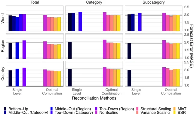
Fig.11showsthemeanabsolutescaledforecast errors(MASE) for all methods, averaged across all forecast dates and horizons.

It mirrors several results obtained from relative RMSFEs seen in the main part. For instance, optimal combinationmethods seem to have, on average, lower forecast errors than the unreconciled

Fig. 11. Mean Absolute Scaled Error of Reconciliation Methods. Lower bars indicate more accurate forecasts. Horizontal lines show the mean absolute scaled error of unreconciled predictions. Errors at intermediate and bottom levels are weighted using their corresponding share in total export volume. Average of all forecast dates and horizons.

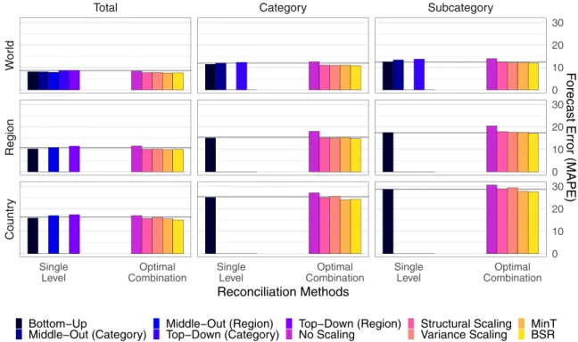
Fig. 12. Mean Absolute Percentage Error of Reconciliation Methods. Lower bars indicate more accurate forecasts. Horizontal lines show the mean absolute percentage error of unreconciled predictions. Errors at intermediate and bottom levels are weighted using their corresponding share in total export volume. Average of all forecast dates and horizons.

Fig. 13. Accuracy of Forecasting Methods at the Top Level. Figure provides several measures of forecast accuracy for the top-level series from 1995 to 2015. Average of all forecast horizons.

benchmark,indicatedby thehorizontalline.Thisholdstrueespe- ciallyforhigherlevels.Single-levelmethodsareoftenlessaccurate thanthebenchmark.Inaddition,top-downandmiddle-outmeth- ods are not able toreconcile grouped hierarchies.At the bottom level, optimalcombinationmethods are,on average,not asaccu- rateastheunreconciledforecastswhenusingtheMASEasamet- ricforforecastingaccuracy.Thisstandsincontrastwiththeresults obtainedfromthe RMSFE, wheremostcombinationmethods im- prove upon the accuracy of unreconciledforecasts at the lowest level.

Fig.12evaluatesthemeanabsolutepercentageerror(MAPE)of reconciledforecastsandcomparesthe resultstotheunreconciled benchmark,againhighlightedusingahorizontalline.Whilethere- sultsareherelessobviousthanintheRMSFEorMASEcase, they stillpointtowardsthesameconclusions:Single-levelmethods,on average, do not outperform the accuracy ofunreconciled predic- tions. Combinationmethods on theother hand,and inparticular MintandBSR,havelowerforecasterrors.

As the forecasting exercises in Section 4 rely on base fore- casts from ARIMA models, it is necessary to also consider

Fig. 14. Accuracy of Forecasting Methods at the Bottom Level. Figure provides several measures of forecast accuracy for the bottom-level series from 1995 to 2015. Average of all forecast horizons. Prediction errors are weighted using their corresponding export shares.

Fig. 15. Composition of Swiss Goods Exports. Treemap shows hierarchical composition of Swiss exports by category and destination in 1988 and 2018.

alternative forecasting methods. However, as the focus of this paper is on the advantages of reconciliation rather than export forecasts, the quality of the underlying base forecasts is not our primary consideration. However, for robustness we consider results from alternative established methods implemented in the ‘hts’ and ’forecast’ packages for R (Hyndman et al., 2011;

Hyndman&Khandakar,2008).

Fig.13showstheforecastaccuracyofARIMAmodelscompared to exponential smoothing state-space models (ETS) andseasonal

random walk models (RW). It shows the average accuracy at eachforecastedperiodfrom1995to2015forthetoplevelseries, measured using all previously established metrics. While there are some differences in the accuracy of the different forecasting methods, the accuracy measures show a very similar picture.

The random walk forecast is very volatile and generally doesn’t outperform the ARIMA and ETS predictions, with the notable exception of the period during the Great Recession. ARIMA and ETSperformverysimilarly.