Impact of Intraseasonal Waves on Angolan Warm and Cold Events

1. Introduction

The Angolan upwelling system as part of the tropical eastern boundary upwelling system, is a highly pro- ductive ecosystem (Binet et al., 2001; Jarre et al., 2015). The warm Angola Current connects the equatorial Atlantic with the Angolan and Benguela upwelling systems by transporting warm tropical waters southward (Rouault, 2012; Tchipalanga et al., 2018) which can be linked to coastal extreme warm events the so-called Benguela Niños (Imbol Koungue et al., 2017, 2019; Mercier et al., 2003; Rouault et al., 2007, 2018; Shan- non et al., 1986). Benguela Niñas are the opposite of Benguela Niños (Imbol Koungue et al., 2017, 2019).

These extreme coastal warm and cold events usually peak in late austral summer between March and April (Florenchie et al., 2003, 2004; Imbol Koungue et al., 2017, 2019; Lübbecke et al., 2010; Rouault et al., 2007).

They are of great socioeconomic importance for the countries of Southern Africa due to their impacts on the marine ecosystem, biological productivity, and fisheries as they modulate the upwelling intensity and upper-ocean mixing thereby setting the upward supply of nutrients (Blamey et al., 2015; Boyer et al., 2001).

They also affect the regional climate and rainfall (Hansingo & Reason, 2009; Koseki & Imbol Koungue, 2021;

Rouault et al., 2003) causing flooding or drought in the neighboring countries. There might be an impact of

Abstract

The intraseasonal variability of the tropical eastern boundary upwelling region in the Atlantic Ocean is investigated using multiyear mooring and satellite data. Pronounced oscillations of alongshore velocity and sea level off Angola at periods of about 90 and 120 days are observed. Similar spectral peaks are detected along the equator suggesting an equatorial forcing via equatorial and coastally trapped waves. Equatorial variability at 90 days is enhanced only in the eastern Atlantic likely forced by local zonal wind fluctuations. Variability at 120 days is generally stronger and linked to a second equatorial basin mode covering the whole equatorial basin. Besides forcing of the 120-day variability by equatorial zonal winds, additional forcing of the resonant basin mode likely originates in the central and western tropical North Atlantic. The coastally trapped waves generated at the eastern boundary by the impinging equatorial Kelvin waves that are detected through their variations in sea level anomaly are associated with corresponding sea surface temperature anomalies delayed by about 14 days. Off Angola, those intraseasonal waves interfere with major coastal warm and cold events that occur every few years by either enhancing them as for the Benguela Niño in 1995 or damping them as for the warm event in 2001.

Plain Language Summary

The tropical Angolan upwelling system hosts a highly productive ecosystem which plays a key socioeconomic role for societal development and fisheries in Angola. The eastern boundary circulation off Angola is dominated by the warm poleward-flowing Angola Current.

During austral summer, the Angola Current transports warm tropical waters into the Benguela upwelling system. Such a transport is often linked to extreme coastal warm events the so-called Benguela Niños.

The opposite of Benguela Niños are Benguela Niñas, both affecting the marine ecosystem and climate on multiyear time scale. At intraseasonal time scale, the Angola Current variability is dominated at periods of 90 and 120 days emanating from equatorial forcing. The 120-day variability in the equatorial basin resembles a resonance of east- and westward-propagating waves. This resonant basin mode transmits part of its energy poleward as coastally trapped waves forcing the variability along the Angolan coast and at the northern boundary of the Gulf of Guinea. The impact of these intraseasonal waves on the development of the extreme coastal warm or cold events can be shown by the relation between sea level and sea surface temperature anomalies in Southern Angola: maximum sea level is leading maximum sea surface temperature by about 14 days.

© 2021. The Authors.

This is an open access article under the terms of the Creative Commons Attribution License, which permits use, distribution and reproduction in any medium, provided the original work is properly cited.

Impact of Intraseasonal Waves on Angolan Warm and Cold Events

Rodrigue Anicet Imbol Koungue¹ and Peter Brandt^1,2

1GEOMAR Helmholtz Centre for Ocean Research Kiel, Kiel, Germany, ²Christian-Albrechts-Universität zu Kiel, Kiel, Germany

Key Points:

• Intraseasonal variability of the Angola Current is linked to equatorial ocean dynamics and interfere with Benguela Niños and Niñas

• Coastally trapped waves off Angola at 120-day period are associated with equatorial basin-mode resonance

• Intraseasonal coastally trapped waves impact sea surface temperature off Angola and in the Gulf of Guinea via thermocline feedback

Supporting Information:

Supporting Information may be found in the online version of this article.

Correspondence to:

R. A. Imbol Koungue, rodrigueanicet@gmail.com

Citation:

Imbol Koungue, R. A., & Brandt, P.

(2021). Impact of intraseasonal waves on Angolan warm and cold events.

Journal of Geophysical Research:

Oceans, 126, e2020JC017088. https://

doi.org/10.1029/2020JC017088 Received 15 DEC 2020 Accepted 30 MAR 2021

10.1029/2020JC017088

RESEARCH ARTICLE

climate warming or multidecadal variability on Benguela Niños as well. Recently, in the Atlantic Ocean, it was shown that the variability of the sea surface temperature (SST) along the equator (in May–June–July, Prigent, Lübbecke, et al., 2020) and in the southeast Atlantic Ocean (in March–April–May, Prigent, Imbol Koungue, et al., 2020) has undergone a reduction by more than 30% at interannual time scale in the post- 2000 period compared to 1982–1999.

The Angola Current variability is mostly controlled by coastally trapped waves (CTWs) either remotely forced by equatorial Kelvin waves (EKWs) impinging at the eastern boundary or locally by the alongshore wind (Bachèlery et al., 2016, 2020; Illig & Bachèlery, 2019; Illig et al., 2018; Kopte et al., 2017; Ostrowski et al., 2009; Rouault, 2012). Polo et al. (2008) studied the propagation of intraseasonal waves with periods ranging from 25 to 95 days along the equatorial and coastal wave guides using altimetric sea level data. They found part of the wave energy to be phase-locked to the seasonal cycle (their Figure 6a) with downwelling wave passage observed in September and December and upwelling wave passage during November and January. Also, Kopte et al. (2018) identified distinct peaks of variability at intraseasonal time scale (about 90, 100, and 120 days) in moored velocity data off Angola. Likely, they detected elevated energy at 120 days in the zonal velocities at 23°W at the equator and suggested a resonance of either the gravest equatorial basin mode of the first baroclinic mode or the second equatorial basin mode of the second baroclinic mode.

According to Cane & Moore (1981), an equatorial basin mode is defined as low-frequency standing equato- rial wave mode which is solely constituted of an eastward-propagating EKW and a westward-propagating long equatorial Rossby wave (ERW) of a specific baroclinic mode covering the whole equatorial basin. The condition for resonance is defined as

,  4

m n n

T L

(1)mc

where T is the resonance period, L is the basin width (5.8 × 10⁶ m), m represents the rank of the equatori- al basin mode (for instance m = 1 is the gravest basin mode), and cⁿ is the gravity phase speed of the nth baroclinic mode (Fu, 2007; Han et al., 2011; Kopte et al., 2018). The equatorial basin mode is not a normal mode as it leaks energy toward higher latitudes by means of CTWs (e.g., Han et al., 2011). In the equatorial Atlantic, the gravest equatorial basin mode has been mostly studied (Brandt et al., 2016; Ding et al., 2009;

Greatbatch et al., 2012; Thierry et al., 2004) with only few indications of the existence of higher order basin modes (Kopte et al., 2018). According to Cane and Sarachik (1981) and Cane & Moore (1981), the interfer- ence pattern resulting from the superposition of an EKW and its eastern boundary-reflected Rossby wave (RW) is characterized by maxima of zonal velocity at

 



   2 1 4 ⁿ

e c

x x k

(2)

where x^e is the longitude of the eastern boundary and k 0,1, 2, is a positive integer (see Cane & Sara- chik, 1981; Han et al., 2011). Note that under resonant conditions given by Equation 1 for m = 1, Equation 2 yields a maximum of zonal velocity amplitude in midbasin, i.e. at x x eL/ 2.

Hughes et al. (2016) have identified an off-equatorial basin-mode resonance at 120-day period in the Car- ibbean Sea basin excited by baroclinic instability of the Caribbean Current. This basin mode is composed of westward-propagating RWs and reflected CTWs propagating eastward along the southern boundary. It is likely that the Caribbean Sea basin mode leaks energy through CTWs reaching the equator and via propa- gation along the equatorial and eastern boundary coastal wave guides impacts the eastern boundary circu- lation off Angola and in the Gulf of Guinea (Hughes et al., 2019).

The present paper aims at studying the superposition of intraseasonal waves on lower-frequency varia- bility and their impact on the SST off Angola. It is structured as follows: Section 2 describes the data and methods used for the analyses. Section 3 presents the main results from the description of the intraseasonal variability at 11°S to its impact on the SST in the Angola-Benguela upwelling system. Section 4 will provide discussion of the analyses and conclusion.

Journal of Geophysical Research: Oceans

2. Data and Methods

2.1. Data

2.1.1. Moored Velocities

The observed Angola Current velocities are obtained from a current meter mooring deployed off Angola (13°00′E; 10°50′S) since July 23, 2013 (Kopte et al., 2017). The mooring is located at around 77 km away from the coast at around 1,200-m depth on the continental slope. On the mooring cable, at 500-m depth, an upward-looking 75-kHz Long Ranger acoustic Doppler current profiler (ADCP) is mounted to measure the velocity of the Angola Current up to 45 m below the sea surface with a 16-m bin size as vertical resolution.

The mooring has come accidentally to the surface in July 2019 and was redeployed in September 2019.

Current velocities from the moored ADCP are rotated by −34° against North to derive alongshore and cross- shore velocities (positive on-shore) according to the local coastal orientation.

We also use ocean current velocities from equatorial moorings located at 35°W, 23°W, 10°W, and 0°E. For each of these four moorings, details about the length of their time series in the upper 500 m are represented in Figure 1. At 35°W, 0°N, there is a moored ADCP covering the upper 550-m depth recording velocities between August 2004 and June 2006 (Hormann & Brandt, 2009). The equatorial zonal current measure- ments at 23°W, 0°N are given by a combination of two moored ADCPs which are recording the velocities in the upper 600–900 m between 2004 and 2019. Details about this equatorial mooring could be found in Brandt et al. (2016). Regarding the current velocity measurements at 10°W, 0°N, we have used data from the PIRATA (Prediction and Research Moored Array in the Tropical Atlantic; Bourlès et al., 2008, 2019;

Johns et al., 2014; Servain et al., 1998) program consisting of a moored ADCP data sampling in the upper 300 m between 2006 and 2019. Since 2016, a moored ADCP located at 0°E, 0°N from the PIRATA program is sampling the equatorial current velocities in the upper 300 m. More details about the PIRATA moorings could be found in Bourlès et al. (2019).

2.1.2. Optimum Interpolation SST Version 2

The daily Optimum Interpolation SST version 2 (OI-SST v2; Reynolds et al., 2007) available at 0.25° hori- zontal resolution from September 1981 onward is used. Data can be downloaded from the NOAA website (https://www.esrl.noaa.gov/psd/data/gridded/). The data are derived from daily merged in situ and remote sensed data.

2.1.3. Altimetry

The gridded products of sea level anomaly (SLA), absolute dynamic topography, and the near-surface ab- solute geostrophic current velocities from the delayed-time multimission (all-sat-merged) are distributed by the EU Copernicus Marine Service Information (http://marine.copernicus.eu/) on a daily temporal resolution and available on a 0.25° horizontal resolution from January 1993 to May 2019. Refer to Pujol et al. (2016) for more details on the mapping algorithm procedures. To complement the moored velocity time series, absolute geostrophic current velocities are extracted from the data point (13°07.5′E; 10°52.5′S) closest to the mooring position as in Kopte et al. (2018).

2.2. Methods

The equatorial zonal geostrophic velocity (Ueg) was estimated by fitting a second-order polynomial func- tion in latitude to the daily absolute dynamic topography data between 1°S and 1°N and evaluating equato- rial geostrophy as in Brandt et al. (2011). Part of the velocity variability found at the equator is related to ba- sin-mode oscillations (see e.g., Brandt et al., 2016; Kopte et al., 2018) and these basin-mode oscillations are typically well described by harmonic oscillations (Cane & Moore, 1981; Claus et al., 2016). For that reason, in this study, a harmonic analysis is used for specific periods to highlight the possible basin-mode character of the variability at 90 and 120 days. The 90- and 120-day harmonic fits (H90 and H120, respectively) are applied to parameters (e.g., Ueg and SLA between 1993 and 2018) using a linear regression model in a least squares sense given by

   

     

   cos  sin

d g I t t

(3) 10.1029/2020JC017088

where dm is the fitted data set;  a column vector constituted of scalar model factors _1, _{2, and} ₃; g represents the linear regression model ma- trix used in the harmonic fits which is composed of three columns: The identity matrix (I), the cosine and sine of t with t the time vector and  the angular frequency ( 2

T ) with T the corresponding period of the harmonic fit. The amplitude, a, and the phase, , of the harmonic oscilla- tion are defined by a ₂²₃² and ^{ }atan2



^{ }3 2,



.

The corresponding error matrix (_Δ) associated with the harmonic cal- culations is then derived using the formula:

  ^{   }



  

 

1

Δ

T T

m m

g g d d d d

(4)n k

where n is the number of degrees of freedom calculated by dividing the length of the time series by a quarter of the period used for the fit;

k represents the number of dependent model factors, here assumed to be 2. In Equation 4, d is the original data set. In this case, the diagonal elements of _Δ give the standard errors of the elements of . The final amplitude errors are then derived using linear error propagation. The same method was used in Brandt et al. (2011). Standard errors of the amplitude and phase of the H120 performed using 3-year running win- dow to SLA (22°W–12°W; 1°S–1°N) and Ueg (5°W–0°E) are estimated by the standard deviations of the amplitudes and phases divided by the square root of 8 (the number of independent values). To investigate the intraseasonal variability in the SLA and SST, we apply a band pass But- terworth filter of sixth order between 75 and 135 days. Also, the wind components (zonal, meridional) and the derived wind stress curl are regressed onto SLA for the Southern Angola region (10°S–15°S, from the coast to 1° offshore). Prior to the regressions, derived SLA time series are band pass filtered between 81–99 days and 108–132 days to closely investigate the equatorial versus eastern boundary forcing of the corresponding intraseasonal waves. A Hilbert empirical orthogonal func- tion (HEOF) is derived from the SLA time series for the eastern tropical Atlantic (0°–20°E; 15°S–5°N) that was band pass filtered between 75 and 135 days to illustrate the intraseasonal CTW propagations between 1993 and 2018.

3. Results

3.1. Intraseasonal Variability in the Angola Current

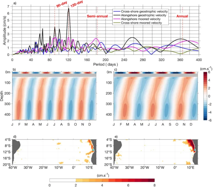
To identify the dominant periods of variability in the direct velocity measurements from the mooring at 11°S and in the corresponding absolute geostrophic surface velocities, harmonic fits are applied (Equa- tion 3). Derived periodograms of moored velocities at each depth level (between 45 and 450 m) are then vertically averaged and shown together with the periodogram of the absolute geostrophic surface velocities (Figure 2a). As already identified in Kopte et al. (2018) for the alongshore flow from the mooring off Angola, peaks of variability are observed at about the annual (∼2 cm/s), semiannual (∼2.3 cm/s), and at intrasea- sonal time scale (period <150 days) with prevailing periods of 90 and 120 days and amplitudes of about 2.5 cm/s each. Those peaks of variability are also present in the absolute alongshore geostrophic surface velocity from altimetry with higher amplitudes, whereas they are absent in the cross-shore components (altimetry and mooring). The remaining of the paper will be dedicated to the description of the variability at 90- and 120-day periods.

The vertical structure in the alongshore velocity for the 90-day (120-day) variability is shown in Figure 2b (2c). Interestingly, the 120-day variability has a higher baroclinicity than the 90-day one, which can be iden- tified by the stronger inclination with depth of the velocity signal. The higher baroclinicity in the 120-day Figure 1. Length of available time series of zonal velocities as function

of depth for equatorial moorings at 35°W (green), 23°W (red), 10°W (black), and 0°E (magenta). Each vertical profile corresponds to a mooring position.

Journal of Geophysical Research: Oceans

variability (Figure 2c) could be identified by the strong change in the amplitude of the alongshore current from near the surface to subsurface, meaning that the 120-day variability is likely associated with higher baroclinic mode waves than the 90-day variability. Large amplitudes (>4 cm/s) of the H90 and of the H120 (>7 cm/s) of the absolute meridional geostrophic surface velocities from altimetry south of the equator are found along the southwest African coast north of Angola-Benguela frontal zone (Figures 2d and 2e), which is located between 15°S and 18°S (Lass et al., 2000; Shannon et al., 1987; Tchipalanga et al., 2018).

The corresponding phase (not shown) portrays a poleward phase increase corresponding to poleward CTW propagations indicating that part of the intraseasonal variability at 90- and 120-day periods originates in the equatorial Atlantic.

10.1029/2020JC017088

Figure 2. (a) Vertically averaged periodograms of moored velocities (cross-shore and alongshore components) between 45 and 450 m and periodogram of absolute geostrophic surface velocity from altimetry (cross-shore and alongshore components) at the mooring position. (b) H90 of the alongshore velocities (absolute geostrophic velocities at the surface and moored velocities at subsurface) shown for a full year. (c) Same as (b), but for H120. (d) H90 of the meridional absolute geostrophic velocity in the tropical South Atlantic. (e) Same as (d), but for H120. All results are derived for the mooring period from July 22, 2013 to June 14, 2019. The cyan square in (d and e) represents the mooring position.

3.2. Equatorial Variability at 90- and 120-Day Periods

The spatial and temporal structure of the 90- and 120-day harmonic fits (cf., Section 2.2) of Ueg and SLA along the equator as calculated using data from January 1993 to December 2018 is presented in Figure 3.

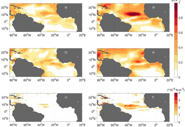
At 90-day period, high amplitude oscillations of SLA (>0.5 cm) and Ueg (>2 cm/s) are collocated in space and time in the eastern equatorial Atlantic (east of about 6°W, Figure 3a). These in phase oscillations, with maximum SLA occurring simultaneously with maximum Ueg, indicate propagating wind-forced equatorial waves. Moreover, the H90 of zonal wind from the Cross-Calibrated Multi-Platform version 2 (CCMPV2, At- las et al., 2011) in the tropical Atlantic (Figure 4a) reveals the presence of enhanced amplitudes (>0.2 m/s) in the eastern equatorial Atlantic. Hence, the equatorial forcing through wind-forced EKW impinging at the eastern boundary and subsequent poleward CTW propagation contributes to generate the 90-day variability in the observed alongshore velocity off Angola. This finding is supported by the recent study from Illig and Bachèlery (2019) highlighting the role played by wind-forced EKW and subsequent poleward CTW of pe- riods less than 120 days along the West African coast. In addition, the H90 amplitude of Ueg in the eastern equatorial Atlantic portrays strong fluctuations. Low amplitude (<2 cm/s) is recorded at around 6°W, while larger amplitudes are observed at around 1°E (>5 cm/s) and at 13°W (>4 cm/s) (Figure 3c). This behavior Figure 3. (a) H90 of Ueg (SLA) in color shading (contours in cm) along the equator shown for a full year; (b) same as (a), but for the H120. (c) Amplitude of the H90 of Ueg (in blue) and SLA (in black) and their associated amplitude errors (cf., Section 2.2) given by the colored shaded areas, respectively. These results are derived from January 1993 to December 2018. A one-degree running mean is applied to the harmonic amplitudes of SLA and Ueg. The colored dots represent the vertically averaged (10–45 m) amplitudes of the H90 of the equatorial zonal velocity measured at the equatorial moorings. Their associated amplitude errors are given by the error bars; (d) same as (c), but for the H120. The equatorial mooring positions are represented by the colored triangles on top of panels (c and d) (35°W in green, 23°W in red, 10°W in black, and 0°E in magenta). The lengths of the mooring time series available to perform the harmonic analysis are represented in Figure 1.

Journal of Geophysical Research: Oceans

is further discussed in Section 4. At 90-day period, a resonant equatorial basin mode covering the whole equatorial basin cannot be observed. To get further evidence of the equatorial velocity variability, the verti- cally averaged (10–45 m) H90 amplitudes of the equatorial zonal velocities measured at different mooring positions along the equator are computed and shown in Figure 3c.

This depth range (10–45 m) is chosen as it allows to stay above the core of the equatorial undercurrent.

The smallest vertically averaged amplitude of the H90 of zonal velocity from the four equatorial moorings is derived at 23°W (1.08 ± 1.60 cm/s), which is consistent with the relatively small H90 amplitudes of Ueg (<2 cm/s) at 23°W (Figure 3a). Larger H90 amplitudes are found in the eastern equatorial Atlantic at 10°W (5.56 ± 2.91 cm/s) and 0°E (2.80 ± 7.48 cm/s), which is in general agreement with the distribution of the H90 amplitude of Ueg. However, contrary to the weak H90 amplitudes of Ueg in the western equatorial Atlantic (Figure 3a), a large H90 amplitude (5.03 ± 2.21 cm/s) is derived from moored velocities at 35°W (Figure 3c). Note that, at 35°W, the mooring data from 10- to 45-m depth are available between August 2004 and June 2006. To test the possibility of interannual variability of the H90 amplitudes, overlapping 3-year periods of Ueg are evaluated. Between 1993 and 2018, the H90 amplitude of the Ueg averaged around the mooring position (between 40°W and 30°W) shows indeed an enhanced amplitude during 2004–2006 of 2.8 cm/s compared to the mean amplitude (1.98 ± 0.31 cm/s) indicating that the mooring deployment at 35°W likely was during a period of an anomalously strong zonal velocity variability at 90-day period.

The 120-day variability of Ueg instead reveals a basin-filling pattern with two amplitude maxima (>6 cm/s) in the western and eastern equatorial Atlantic separated by a minimum (<2 cm/s) in the middle of the basin

10.1029/2020JC017088

Figure 4. Amplitude of H90 between July 2013 and April 2019 of CCMP (a) zonal wind; (b) meridional wind; (c) estimated wind stress curl. (d–f) Same as in (a–c), but for H120.

and small values at the eastern and western boundaries (Figures 3b and 3d). Conversely, the pattern of the 120-day variability of SLA, while also showing a basin-filling pattern, has minima in the western (<0.2 cm) and eastern (<0.6 cm) equatorial Atlantic separated by a maximum (>1 cm) in the middle of the basin as well as large values at the eastern and western boundaries (Figures 3b and 3d). These spatially out phase patterns of maxima and minima in the H120 amplitude of SLA and Ueg (Figures 3b and 3d) resemble that of a second equatorial basin mode previously described for the intraseasonal variability in the Indian Ocean (see e.g., Fu, 2007; Han et al., 2011). The vertically averaged (10–45 m) H120 amplitudes of the equatorial zonal velocities at the mooring positions show larger values (>10 cm/s) in the eastern (0°, 10°W) and small- er values (<6 cm/s) in the western Atlantic (23°W, 35°W, Figure 3d), which indicate only weak correspond- ence between H120 amplitudes of moored velocities and Ueg.

The resonant condition (Equation 1) for the second equatorial basin mode of the second baroclinic mode is just the period of the gravest equatorial basin mode of the second baroclinic mode divided by two (see Brandt et al., 2016, their Table 1 for n = 2) which is around 102 days. Brandt et al. (2016) found a resonance period of 109 days for the gravest equatorial basin mode of the first baroclinic mode. Although the reso- nance period of that basin mode is closer to 120 days, the gravest basin mode could not be identified in the H120 amplitude of Ueg and SLA. Also, at 23°W, the H120 amplitude of moored velocities does not suggest the presence of enhanced first baroclinic mode waves (Kopte et al., 2018). An explanation could be that the forcing at the 120-day period overwhelmingly generates second baroclinic mode waves with first baroclinic mode waves not energetic enough to form a resonant basin mode or too incoherent with respect to the sea- sonal cycle. Unfortunately, direct velocity measurements at other equatorial moorings than 23°W (where the second basin mode is close to its minimum zonal velocity amplitude) do not cover the full depth range (Figure 1) and a dominance of the second baroclinic mode for H120 amplitude of moored velocities cannot be proven at these locations.

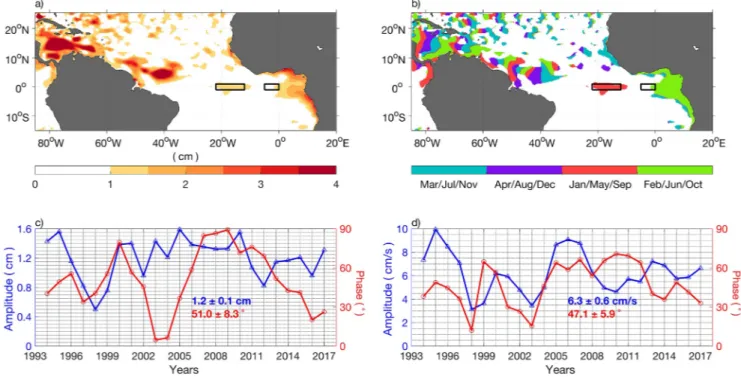
Figure 5. (a) Amplitude and (b) phase of the H120 of SLA between 2003 and 2007. Phase corresponds to the maximum sea level elevation. White areas in the phase map represent areas where the amplitude is less than 1 cm. (c) Evolution of amplitude (blue) and phase (red) of H120 of SLA averaged between 22°W–12°W and 1°S-1°N (big black box marked in (a) and (b)) calculated from 3-year long overlapping time series for the period 1993–2018. (d) Same as in (c), but for Ueg averaged between 5°W and 0°E along the equator (small black box marked in (a) and (b)). Regions used in (c) and (d) are regions of high H120 amplitudes of SLA and Ueg, respectively, identified in Figure 3d. Phases from 0° to 90° correspond to the months January or May or September, respectively (cf., Figure 5b). Details about the calculation of standard errors of the amplitude and phase of the H120 of SLA in (c) and Ueg in (d) are given in Section 2.2.

Journal of Geophysical Research: Oceans

Figure 5a (5b) illustrates the horizontal structure of the amplitude (phase) of the H120 of SLA calculated for the period 2003–2007 in the tropical Atlantic. This period is chosen randomly since the patterns are con- sistent with those derived for other 5-year windows. Patterns of the H120 of SLA along the equator show high amplitudes in the middle of the basin and at the western and eastern boundaries which match well the amplitude distribution shown in Figures 3b and 3d. Furthermore, high H120 amplitudes (>2 cm) of SLA are observed along the West African coast (Figure 5a) and associated with phases ranging between 90°

and 180° which correspond to the months February or June or October (Figure 5b). The high amplitudes (>2 cm) at the eastern boundary are consistent with CTW propagations (poleward away from the equator).

South of the equator, they impact the eastern boundary circulation off Angola as identified in the moored velocity records taken at 11°S (Figure 2a). The radiation of westward-propagating RWs generated at the eastern boundary associated with poleward CTW propagations is only weakly indicated by the westward increase of the phase of the H120 along the West African coast (Figure 5b).

Figures 5c and 5d show the evolution of amplitude and phase of the H120 of SLA and Ueg averaged in the regions of maximum H120 amplitude represented by the two black boxes in Figures 5a and 5b, respectively.

It is interesting to note that the amplitude and phase calculated for overlapping 3-year periods remain rela- tively constant from 1993 to 2018. A constant phase would indicate that the 120-day oscillations are phase- locked to the seasonal cycle. For the 120-day variability of the SLA (Figure 5c), a mean phase of 51 ± 8.3°

corresponds to maximum SLA occurring either January or May or September 17, ±3 days, whereas for the Ueg (Figure 5d), a mean phase of 47.1 ± 5.1° corresponds to maximum Ueg occurring either January or May or September 16, ±2 days. As the 120-day variability is dominated by the second basin mode and the annual and semiannual variability by the gravest basin modes (Brandt et al., 2016), the 120-day variability of SLA and Ueg along the equator is particularly strong in regions, where the annual and semiannual variability of SLA and Ueg is weak.

10.1029/2020JC017088

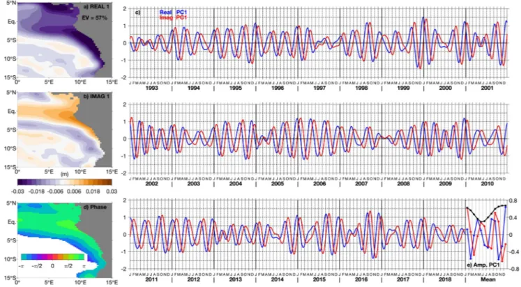
Figure 6. First HEOF mode of the SLA band pass filtered between 75 and 135 days in the eastern tropical Atlantic between 0°E–20°E and 15°S–5°N from 1993 to 2018: (a) real and (b) imaginary spatial patterns; (c) real (blue) and imaginary (red) principal components of the first HEOF (PC1); (d) relative phase associated with the spatial patterns. Note that the phase differences in (d) must be interpreted with regard to the instantaneous oscillation period;

for a dominant period of 120 days, a phase difference of _{/ 2} corresponds to 30 days. (e) Mean seasonal cycles of real (blue) and imaginary (red) principal components of the PC1 and amplitude of the PC1 = 



^{Real PC12ImagPC12}



^{in black.}

The same analyses for SLA and Ueg have been conducted for the 90-day variability along the equator (not shown). Here, we chose the region between 5°W and 5°E, in which the H90 amplitudes of SLA and Ueg are both maximum (Figure 3c). For the 90-day oscillations, maximum SLA is found at a mean phase of 146.51 ± 10.32° corresponding to either February or May or August or November 7, ±3 days and maximum Ueg at 122.33 ± 12.37° corresponding to February or May or August or November 1, ±3 days. The obtained variations of the phases indicate that the 90-day oscillations are less phase-locked to the seasonal cycle along the equator than the 120-day oscillations.

3.3. Impacts on the SST Variability

To identify the dominant intraseasonal variability of SLA, we calculate HEOFs of SLA band pass filtered between 75 and 135 days. The real and imaginary patterns of the first HEOF mode explain 57% of the vari- ance of the SLA data (Figures 6a and 6b). Strong amplitudes (>2 cm) are observed at the eastern boundary and are associated with poleward-increasing phases as can be observed in Figure 6d, mainly north of the Angola-Benguela frontal zone and along the northern boundary of the Gulf of Guinea.

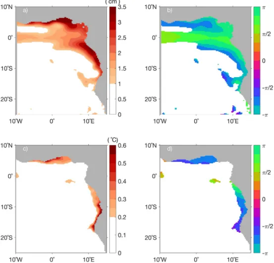
Such phase changes are reminiscent to CTW propagations, whereas positive SLA is associated with down- welling waves and negative SLA with upwelling waves. Figure 6c shows the variations in time of the real and imaginary principal components of the first HEOF mode (PC1). During most years, the PC1 is dominat- Figure 7. (a) Amplitude and (b) phase of intraseasonal oscillations calculated from the real and imaginary linear regression patterns that are derived by regressing the SLA band pass filtered between 75 and 135 days onto the PC of the first HEOF of SLA calculated between 0°E–20°E and 15°S–5°N from 1993 to 2018 (cf., Figure 6c). (c) and (d) Similarly calculated to (a) and (b) but are obtained by regressing SST anomalies.

Journal of Geophysical Research: Oceans

ed by 120-day oscillations (three oscillations per year), however, with remarkable year-to-year variations in the amplitude of the intraseasonal variability. The mean seasonal cycle of the real and imaginary PC1 (blue and red curves respectively in Figure 6e) also displays a dominance of the 120-day oscillations with for in- stance downwelling waves propagating in February, June/July, and October for the real PC1. Furthermore, the mean seasonal cycle of the amplitude of the PC1 (black curve in Figure 6e) depicts minimum amplitude during April–July (particularly including the phase of downwelling wave propagation in June/July) and maximum in November–February.

The identified 120-day oscillations contribute to the seasonal cycle of upwelling and downwelling waves along the Angolan coast. Seasonal variations of the SLA are dominated by a semiannual cycle with down- welling waves occurring in February/March and October/November; the SLA amplitude of the semian- nual cycle is about 5 cm (Rouault, 2012; Zeng et al., 2021, their Figure 1c). The amplitude of the intra- seasonal variability might reach more than 3 cm and substantially contribute to SLA variations during some years. The part of the intraseasonal variability that is phase-locked to the seasonal cycle (Figure 6e) still reach amplitudes of about 1.06 cm and thus contributes up to about 20% to the SLA seasonal cycle. It strengthens the seasonal downwelling in February and October and weakens the upwelling in June/July.

The main upwelling season of Angola is in July–September (Kopte et al., 2017; Ostrowski et al., 2009; Zeng et al., 2021). This upwelling signal is again strengthened in its later phase by the upwelling wave of the phase-locked 120-day oscillations peaking in August/September.

10.1029/2020JC017088

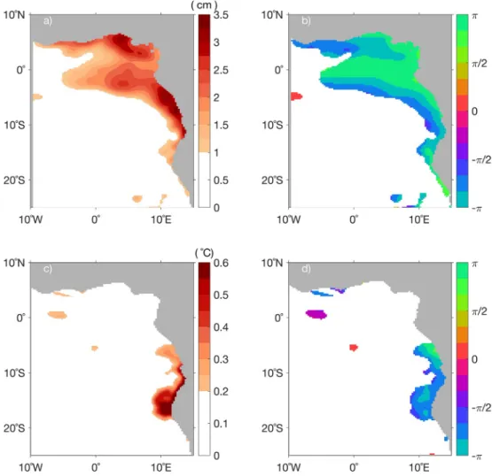
Figure 8. (a) Amplitude and (b) phase of intraseasonal oscillations calculated from the real and imaginary linear regression patterns that are derived by regressing SLA band pass filtered between 75 and 135 days onto the PC of the first HEOF of SLA calculated between 0°E–20°E and 15°S–5°N from 1993 to 2018 (cf., Figure 6c) only for JFM. (c) and (d) Similarly calculated as (a) and (b) but are obtained by regressing the band pass filtered SST anomalies for JFM.

Next, we want to study the impact of the intraseasonal waves on the SST. This is done by calculating regres- sions of SLA and SST anomalies onto the real and imaginary PC of the first HEOF of intraseasonal SLA variability shown in Figure 6c. Figures 7a and 7b show the amplitude and phase of the regressed SLA. Note that the phase shown in Figure 7b is essential the same as shown in Figure 6d.

Regression results show large amplitudes (>3 cm) near the coast north of the Angola-Benguela frontal zone and along the northern boundary of the Gulf of Guinea, which is consistent with the patterns of HEOF analysis of the SLA anomalies shown in Figures 6a and 6b. Phase changes (Figure 7b) indicate poleward CTW propagations along the eastern boundary south of the equator and westward CTW propagations along the northern boundary of the Gulf of Guinea. In comparison to the regression of SLA, Figures 7c and 7d show the regression of SST anomalies onto the same real and imaginary PC of the first HEOF (cf., Fig- ure 6c). The calculated patterns reveal the impact of intraseasonal CTWs with periods ranging between 75 and 135 days on SST. As shown before, this intraseasonal band is dominated by 120-day oscillations (three oscillations per year, cf., Figures 6c and 6e). The intraseasonal CTWs are defined here by their SLA variabili- ty, which can be interpreted as an associated variability in thermocline depth. The impact of these waves on the SST along the African coast can be observed south of the equator between 3°S and 18°S as well as along the northern boundary of the Gulf of Guinea.

The question remains if there is a time difference in the occurrence of maximum SLA and maximum SST associated with the intraseasonal wave propagation. Such a time difference would be indicative of a ther- mocline feedback transferring the signal of a displaced thermocline toward a SST anomaly. Between 10°S and 15°S and from the coast to 1° offshore (Southern Angola region), the mean SLA phase is −173.4° and Figure 9. Same as in Figure 8, but for AMJ.

Journal of Geophysical Research: Oceans

the mean SST phase is −131.0° (cf., Figures 7b and 7d). The resulting phase difference is −42.4°, which corresponds, when assuming a dominance of 120-day variability (three oscillations per year, cf., Figures 6c and 6e), to SLA leading SST by about 14 days. Such a phase lag is at the lower end of the range of phase lags identified in the eastern equatorial Pacific (Zelle et al., 2004; Zhu et al., 2015). It corresponds to a situation with shallow thermocline depths as can be found in general in tropical upwelling regions. The delayed SST response to changes in thermocline depth, i.e. the thermocline feedback, involves atmospherically forced or shear-induced upper-ocean mixing transferring the subsurface signal to the surface. While the link between SLA and SST can be well observed along the Angolan coast and in the northern Gulf of Guinea, it is missing in the northeastern corner of the Gulf of Guinea. This is likely due to the presence of a low-salinity surface layer and correspondingly a stronger near-surface stratification (Berger et al., 2014) that hinders the ther- mocline feedback to be active by damping upper-ocean mixing.

As previous studies showed a dependence of the phase lag between SLA and SST on the background up- per-ocean stratification or the thermocline depth, we expect that the phase lag off Angola varies with the seasonal stratification (Kopte et al., 2017). To study the seasonal variations in the SST response to intrasea- sonal SLA variability, we perform a regression analysis of the band-pass-filtered SST onto the same real and imaginary PC of the first HEOF mode of SLA anomalies, but now for different seasons of the year (Figures 8–11). The band-pass-filtered SST and SLA anomalies are calculated by band pass filtering between 75 and 135 days, subtracting the annual mean of the band-pass-filtered data for the period 1993–2018 and, finally, selecting the different seasons of the year.

10.1029/2020JC017088

Figure 10. Same as in Figure 8, but for JAS.

We find that the most distinct SST propagations associated with CTWs can be observed in January–Febru- ary–March (JFM, Figure 8), which corresponds to the peak period of most Benguela Niño/Niña events (Im- bol Koungue et al., 2019). In JFM (Figure 8), the calculated mean phase difference between SLA and SST in the Southern Angola region is 49.8°. This means that a phase lag of about 17 days for the 120-day variability is estimated when the maximum of SLA (deep thermocline) is leading the maximum of SST. Similarly, the thermocline feedback is active at the northern boundary of the Gulf of Guinea.

Regarding the remaining seasons, the mean phase difference between SLA and SST in the Southern Angola region is 41.52° in April–May–June (AMJ, Figure 9) and 22.86° in July–August–September (JAS, Figure 10) corresponding respectively to around 14 days and around 8 days by which SLA is leading SST. The period JAS corresponds to the upwelling season characterized by a seasonal minimum in thermocline depth off Angola associated with the passage of the seasonal upwelling CTW (Ostrowski et al., 2009; Rouault, 2012).

A comparably large lag of 20 days (mean phase difference between SLA and SST of 60.30°) is found instead in the Southern Angola region for the period October–November–December (OND, Figure 11). During that period, the passage of a seasonal downwelling CTW (Ostrowski et al., 2009; Rouault, 2012) and the presence of low-salinity surface waters (Kopte et al., 2017) is observed that likely explain the delayed response of SST to SLA in comparison to the other seasons.

In a final step, we want to investigate the possible impact of intraseasonal CTWs on the interannual varia- bility off Angola characterized by the presence of extreme warm and cold events, i.e. Benguela Niños/Niñas (Bachèlery et al., 2016, 2020; Imbol Koungue et al., 2017, 2019). A constructive or destructive interference Figure 11. Same as in Figure 8, but for OND.

Journal of Geophysical Research: Oceans

between both processes depends on the amplitude and phase of intraseasonal CTWs and the peak period of Benguela Niño/Niña events. Therefore, the exact timing of the intraseasonal variability might impact the interannual variability or the peaks of the warm/cold events off Southern Angola. The SST response of the intraseasonal waves is estimated as follows: from the mean SLA and SST amplitudes of intraseasonal waves as defined by the regression coefficients given in Figures 7a and 7c, respectively, we can derive an SST response for the Southern Angola region of 0.49°C per 1.92 cm or 0.255°C/cm. This SST response is then multiplied, for different extreme warm and cold events, with the instantaneous SLA value of the in- traseasonal wave (SLA in the Southern Angola region band pass filtered between 75 and 135 days) 2 weeks before the peak of the corresponding event. Table 1 summarizes the impact of intraseasonal CTWs on spe- cific Benguela Niño/Niña events previously identified in Southern Angola by Imbol Koungue et al. (2019, their Table S1) and Lübbecke et al. (2019, for the 2016 warm event). Note that, most of these extreme warm or cold coastal events were previously identified in the recent modeling study of Bachèlery et al. (2020).

The numbers in the fifth column represents the effect of the intraseasonal waves on the specific extreme events. For example, in March 1995, 2 weeks before the peak of the extreme warm event, an intraseasonal downwelling CTW with an amplitude of +2.86 cm is recorded and associated with an increase in the peak SST anomalies of 0.73°C which is around 33% of the peak SST anomaly. The presence of the intraseasonal downwelling wave resulted thus in a strong enhancement of the extreme warm event. Most of the extreme warm or cold events are enhanced by the intraseasonal wave propagation, which seems to be a reasonable result as a damping by intraseasonal waves more likely results in events that are not extreme. However, the 2001 warm event (Rouault et al., 2007) and the 2010 cold event are damped by the presence of intraseasonal waves (cf., Table 1), which suggests that these events would had become more extreme without the presence of intraseasonal waves.

4. Discussion and Conclusions

In this study, the intraseasonal variability of the Angola Current at 11°S and its forcing is analyzed using moored velocity and altimeter sea level data. Enhanced intraseasonal variability (band pass filtered between 75 and 135 days) in alongshore moored velocity data at 11°S are found at 90- and 120-day periods (Fig- ure 2a) with variability at 120-day period dominating (Figure 2e). It is associated with the presence of CTWs propagating poleward along the southwestern African coast north of the Angola-Benguela frontal zone.

10.1029/2020JC017088

Coastal extreme events in Southern

Angola Peak time

(date)

SST anomalies during the peak time (°C)

Band pass filtered SLA anomalies 2 weeks before the

SST peak (cm)

Associated SST anomalies corresponding

to intraseasonal CTWs (°C)

Effects of the intraseasonal

waves

1995 (warm) March 27 +2.23 +2.86 +0.73 Strongly enhanced

1997 (warm) October 28 +1.45 +0.30 +0.08 Enhanced

1998 (warm) June 30 +1.73 +1.45 +0.37 Enhanced

2001 (warm) April 16 +1.73 −0.87 −0.22 Damped

2010 (warm) March 2 +2.05 +1.15 +0.29 Enhanced

2016 (warm) February 20 +1.88 +2.73 +0.70 Enhanced

1997 (cold) April 6 −2.65 −1.49 −0.38 Enhanced

2010 (cold) March 27 −1.57 +0.82 +0.21 Damped

Note. The coastal events were previously identified by Imbol Koungue et al. (2019) except the 2016 warm event, which is described in Lübbecke et al. (2019).

Table 1

Extreme Coastal Warm and Cold Events Which Occurred in the Southern Angola region (10°S–15°S, From the Coast to 1° Offshore) along with the Times of Their Peak SST Anomaly, Their Peak SST Anomaly, the Corresponding SLA Band Pass Filtered Between 75 and 135 Days 2 Weeks Before the SST Peak, the Associated Contributions of Intraseasonal CTWs to the Peak SST Anomalies and the Resulting Effect of the Intraseasonal CTWs During the Coastal Events.

At the 90-day period, the Angola Current variability is mostly linked to equatorial forcing (Figure 4a).

Zonal wind anomalies along the equator east of 20°W force EKW impinging at the eastern boundary of the equatorial Atlantic generating poleward propagating CTW. This scenario agrees with the study of Polo et al. (2008) highlighting continuous and recurrent propagation of EKWs and CTWs at intraseasonal time scale. Also, Illig and Bachèlery (2019) using high-resolution model experiments showed that at subseasonal time scale (∼2–120 days), north of 15°S, CTW modes 1 and 2 dominate the SLA variability (their Figures 2a and 2c). Moreover, 95% statistically significant positive regression coefficients (>15 m/s/m) are derived when the zonal wind fluctuations along the equator lead the SLA anomalies (band pass filtered between 81 and 99 days) averaged in the Southern Angola region by 25 days (Figure S1b). However, forcing at the east- ern boundary associated with alongshore wind fluctuations at 90-day period (Figure 4b) seems not to play a dominant role in the establishment of the 90-day oscillation of the Angola Current as no significant re- gression coefficients were found between the meridional wind anomalies and the band pass filtered SLA off Angola (not shown). Along the equator, the amplitude of the 90-day variability of Ueg (Figures 3a and 3c) shows low amplitude (<2 cm/s) at 6°W and high amplitude (>5 cm/s) at around 13°W and 1°E. Figure 4a also depicts two patches of enhanced H90 amplitude of zonal wind (>0.1 m/s) along the equator (at 20°W and 0°E). We suggest that the phase difference of the equatorial zonal wind forcing at those two locations and then the superposition of directly wind-forced EKWs and ERWs (see Han et al., 2008) could possibly explain the pattern in the 90-day oscillation in the Ueg. At 90-day period, a resonant equatorial basin mode covering the whole equatorial basin as analytically described by Cane & Moore (1981) cannot be observed (Figures 3a and 3c).

Similarly, to the 90-day variability, also at 120-day period, the equatorial forcing contributes to the intra- seasonal variability of the Angola Current. Along the equator, our analyses have shown that intraseasonal CTWs could emanate from the 120-day basin-mode resonance associated with the second equatorial basin mode of the second baroclinic mode. The interference pattern (Equation 2) for the 120-day basin mode fits quite well with results of Figure 3b. Assuming a second baroclinic mode phase speed of 1.32 m/s (Brandt et al., 2016), maximum zonal velocity should occur at 5°W and 36.6°W. About the sources of the 120-day var- iability along the equator, we can only speculate. Figure 5a depicts large H120 amplitudes of SLA (>3.5 cm) in the northwestern tropical Atlantic in two regions: (1) in the Caribbean Sea and (2) the North Equatorial Countercurrent region (around 45°W–30°W; 7°N–9°N). The H120 SLA amplitudes in those two regions are associated with westward-increasing phases (Figure 5b) indicative of the presence of westward-propagating RWs. On the one hand, there is the possibility that the 120-day basin-mode resonance recently identified in the Caribbean Sea basin (Hughes et al., 2016) leaks energy that propagates equatorward as CTWs along the northeast Brazilian coast. It may reach the equator and contribute to the establishment of the 120-day equatorial basin resonance, which finally leaks energy in the form of CTWs and impacts the eastern bound- ary circulation off Angola (see Hughes et al., 2019, their Figure 1). On the other hand, the large amplitude of H120 of SLA (>3.5 cm) observed in the North Equatorial Countercurrent region coincides with an en- hanced H120 amplitude (>2.5 × 10⁻⁸ N/m³) of the wind stress curl (WSC) derived from CCMPV2 winds (Figure 4f) indicating the presence of wind-forced RWs. These long RWs propagate westward reaching the strongly inclined northeast Brazilian coast north of the equator to form CTWs that similarly might reach the equator as described for the leaking energy from the Caribbean Sea basin mode. However, for both process- es, we could not identify a clear signature of CTW propagation along the northeast Brazilian coast. Strong negative regression coefficients (<−0.9 × 10⁻⁶ N/m³/m) are observed in the North Equatorial Countercur- rent region when the WSC anomalies lead the band-pass-filtered SLA anomalies off Southern Angola by 60 days (Figure S1d). This lag of 60 days is a reasonable propagation time for a wind-forced RW in the North Equatorial Countercurrent region to propagate to the western boundary, then as CTW along the northeast Brazilian coast and along the equator as EKW to finally impacting the SLA off Southern Angola through CTW along the southwest African coast. Besides the 120-day equatorial basin resonance and its potential two sources that are not present for the 90-day variability (not shown), the H120 amplitude of the zonal wind (>0.3 m/s) is observed mostly east of 10°W, which highlights a potential contribution from the zonal wind variability at 120-day period in the eastern equatorial Atlantic (Figure 4d). There are also 95% signifi- cant positive regression coefficients (>15 m/s/m) suggesting that zonal wind fluctuations along the equator could trigger EKWs. The EKWs would affect the intraseasonal variability of the SLA off Angola via CTWs when the zonal wind along the equator in the eastern Atlantic is leading by 30 days (Figure S1c). Moreover,

Journal of Geophysical Research: Oceans

the zonal wind forcing in the eastern equatorial Atlantic more directly impacts EKWs and CTWs and is less affected by wave damping as the waveguide for those waves is much shorter than for waves originating in the Caribbean Sea or in the North Equatorial Countercurrent region. Figure 4e also shows enhanced H120 amplitudes of the meridional wind north of 10°S along the southwestern African coast. However, there is no significant regression coefficients observed between the meridional wind anomalies and the band pass filtered SLA off Southern Angola (not shown), indicating that the local forcing at the eastern boundary does not play a dominant role. Note that there is in general a higher amplitude of the wind forcing at 120-day period compared to the 90-day period in the eastern equatorial Atlantic (Figures 4a and 4d) and in the North Equatorial Countercurrent region from WSC (Figures 4c and 4f).

The 120-day equatorial basin resonance shows an east-west asymmetry that is characterized by larger SLA amplitudes in the eastern compared to the western equatorial Atlantic (Figure 3d). A similar east-west asymmetry was previously observed by Han et al. (2011) in the equatorial Indian Ocean for their 90-day second equatorial basin mode of the second baroclinic mode. They explained this asymmetry by the differ- ence in the propagation speeds between the EKW and ERW which leads to a differential mixing with 3 times stronger damping for ERW.

Overall, ocean dynamics at intraseasonal time scale have been evidenced to impact SST variability along the southwestern African coast and in the Gulf of Guinea (Figure 7). The intraseasonal waves are partly phase-locked to the seasonal cycle (Figure 6e, blue and red curves) which is in general agreement with Polo et al. (2008), with downwelling wave passage occurring in Southern Angola in February, June/July, and Oc- tober. Indeed, the mean seasonal cycle of intraseasonal variability off Angola is dominated by the 120-day oscillation (three oscillations per year, Figure 6e (blue and red curves)).

Most of the Benguela Niño/Niña events summarized in Table 1 have their peak almost at the same time as the peak of the intraseasonal CTWs resulting in a predominant enhancement of Benguela Niño/Niña events by intraseasonal CTWs (Table 1). In Southern Angola, we could identify an active thermocline feedback for the 120-day variability with SLA (and thus thermocline depth) of intraseasonal CTW leading SST by around 14 days (cf., Zelle et al., 2004; Zhu et al., 2015). This thermocline feedback, however, is found to be seasonal- ly dependent with slower SST response during austral spring to summer (OND and JFM, deep thermocline seasons) and faster SST response during austral fall to winter (AMJ and JAS, shallow thermocline seasons).

To calculate the impact of intraseasonal waves on Benguela Niño/Niña events, we have assumed that the strength of the SST response to intraseasonal SLA or thermocline anomalies is seasonally independent.

However, it can be expected that the SST response is weaker during periods with deep thermoclines than during periods with shallow thermoclines. Other factors such as the strength of stratification and mixing might play a role as well. A recent modeling study showed that the tidal energy available for mixing at the Angolan shelf is similar throughout the year, albeit the resulting mixing is more efficient during periods of shallow thermocline (Zeng et al., 2021).

Data Availability Statement

The 11°S mooring data set used in this study is publicly available at https://doi.pangaea.de/10.1594/

PANGAEA.909911 and https://doi.pangaea.de/10.1594/PANGAEA.909913 (latest data set is in submis- sion process). The equatorial mooring data at 10°W and 0°E are freely available at https://www.seanoe.

org/data/00404/51557/. The mooring data at 23°W are available at https://doi.pangaea.de/10.1594/PAN- GAEA.924782 and the ones at 35°W at https://doi.pangaea.de/10.1594/PANGAEA.929938. CCMPV2 wind product is available at http://www.remss.com/measurements/ccmp/.

References

Atlas, R., Hoffman, R. N., Ardizzone, J., Leidner, S. M., Jusem, J. C., Smith, D. K., & Gombos, D. (2011). A cross-calibrated, multiplatform ocean surface wind velocity product for meteorological and oceanographic applications. Bulletin of the American Meteorological Society, 92, 157–174. https://doi.org/10.1175/2010BAMS2946.1

Bachèlery, M. L., Illig, S., & Dadou, I. (2016). Interannual variability in the South-East Atlantic Ocean, focusing on the Benguela upwelling system: Remote versus local forcing. Journal of Geophysical Research: Oceans, 121, 284–310. https://doi.org/10.1002/2015JC011168 Bachèlery, M. L., Illig, S., & Rouault, M. (2020). Interannual coastal trapped waves in the Angola-Benguela upwelling system and Benguela

Niño and Niña events. Journal of Marine Systems, 203, 103262. https://doi.org/10.1016/j.jmarsys.2019.103262

10.1029/2020JC017088

Acknowledgments

The research leading to these results received funding from the EU H2020 under grant agreement 817578 TRIAT- LAS project. It was further supported by the German Federal Ministry of Educa- tion and Research as part of the SACUS II (03F0751A), BANINO (03F0795A), and RACE (03F0824C) projects and by the Deutsche Forschungsgemeinschaft as part of the Sonderforschungsbereich 754 Climate–Biogeochemistry Interac- tions in the Tropical Ocean and through several research cruises with RV Maria S. Merian and RV Meteor. We thank the PIRATA project for making the mooring data freely available. We thank the captains, crews, scientists, and technicians involved in several research cruises in the tropical Atlantic who contributed to collecting data used in this study. Open access funding enabled and organized by Projekt DEAL.

Berger, H., Treguier, A. M., Perenne, N., & Talandier, C. (2014). Dynamical contribution to sea surface salinity variations in the eastern Gulf of Guinea based on numerical modelling. Climate Dynamics, 43, 3105–3122. https://doi.org/10.1007/s00382-014-2195-4

Binet, D., Gobert, B., & Maloueki, L. (2001). El Niño-like warm events in the Eastern Atlantic (6°N, 20°S) and fish availability from Congo to Angola (1964–1999). Aquatic Living Resources, 14, 99–113.

Blamey, L. K., Shannon, L. J., Bolton, J. J., Crawford, R. J. M., Dufois, F., Evers-King, H., et al. (2015). Ecosystem change in the southern Benguela and the underlying processes. Journal of Marine Systems, 144, 9–29.

Bourlès, B., Araujo, M., McPhaden, M. J., Brandt, P., Foltz, G. R., Lumpkin, R., et al. (2019). PIRATA: A sustained observing system for tropical Atlantic climate research and forecasting. Earth and Space Science, 6, 577–616. https://doi.org/10.1029/2018EA000428 Bourlès, B., Lumpkin, R., McPhaden, M. J., Hernandez, F., Nobre, P., Campos, E., et al. (2008). The Pirata Program. Bulletin of the American

Meteorological Society, 89(8), 1111–1126. https://doi.org/10.1175/2008BAMS2462.1

Boyer, D. C., Boyer, H. J., Fossen, I., & Kreiner, A. (2001). Changes in abundance of the northern Benguela sardine stock during the decade 1990–2000, with comments on the relative importance of fishing and the environment. South African Journal of Marine Science, 23(1), 67–84. https://doi.org/10.2989/025776101784528854

Brandt, P., Claus, M., Greatbatch, R. J., Kopte, R., Toole, J. M., Johns, W. E., & Böning, C. W. (2016). Annual and semiannual cycle of equatorial Atlantic circulation associated with basin-mode resonance. Journal of Physical Oceanography, 46, 3011–3029. https://doi.

org/10.1175/JPO-D-15-0248.1

Brandt, P., Funk, A., Hormann, V., Dengler, M., Greatbatch, R. J., & Toole, J. M. (2011). Interannual atmospheric variability forced by the deep equatorial Atlantic Ocean. Nature, 473, 497–500. https://doi.org/10.1038/nature10013

Cane, M. A., & Moore, D. W. (1981). A note on low-frequency equatorial basin modes. Journal of Physical Oceanography, 11, 1578–1584.

https://doi.org/10.1175/1520-0485(1981)011<1578:ANOLFE>2.0.CO;2

Cane, M. A., & Sarachik, E. S. (1981). The response of a linear baroclinic equatorial ocean to periodic forcing. Journal of Marine Research, 39, 651–693.

Claus, M., Greatbatch, R. J., Brandt, P., & Toole, J. M. (2016). Forcing of the Atlantic equatorial deep jets derived from observations. Journal of Physical Oceanography, 46, 3549–3562. https://doi.org/10.1175/JPO-D-16-0140.1

Ding, H., Keenlyside, N. S., & Latif, M. (2009). Seasonal cycle in the upper equatorial Atlantic Ocean. Journal of Geophysical Research, 114, C09016. https://doi.org/10.1029/2009JC005418

Florenchie, P., Lutjeharms, J. R., Reason, C. J. C., Masson, S., & Rouault, M. (2003). The source of Benguela Niños in the South Atlantic Ocean. Geophysical Research Letters, 30(10), 1505. https://doi.org/10.1029/2003GL017172

Florenchie, P., Reason, C. J. C., Lutjeharms, J. R. E., Rouault, M., Roy, C., & Masson, S. (2004). Evolution of interannual warm and cold events in the southeast Atlantic Ocean. Journal of Climate, 17(12), 2318–2334. https://doi.org/10.1175/1520-0442(2004)017<2318:EOI WAC>2.0.CO;2

Fu, L.-L. (2007). Intraseasonal variability of the equatorial Indian Ocean observed from sea surface height, wind, and temperature data.

Journal of Physical Oceanography, 37, 188–202. https://doi.org/10.1175/JPO3006.1

Greatbatch, R. J., Brandt, P., Claus, M., Didwischus, S.-H., & Fu, Y. (2012). On the width of the equatorial deep jets. Journal of Physical Oceanography, 42, 1729–1740. https://doi.org/10.1175/JPO-D-11-0238.1

Han, W., McCreary, J. P., Masumoto, Y., Vialard, J., & Duncan, B. (2011). Basin resonances in the equatorial Indian Ocean. Journal of Physical Oceanography, 41, 1252–1270. https://doi.org/10.1175/2011JPO4591.1

Han, W., Webster, P. J., Lin, J.-L., Liu, W. T., Fu, R., Yuan, D., & Hu, A. (2008). Dynamics of intraseasonal sea level and thermocline varia- bility in the equatorial Atlantic during 2002–03. Journal of Physical Oceanography, 38, 945–967. https://doi.org/10.1175/2008JPO3854.1 Hansingo, K., & Reason, C. J. C. (2009). Modelling the atmospheric response over southern Africa to SST forcing in the southeast tropical

Atlantic and southwest subtropical Indian Oceans. International Journal of Climatology, 29(7), 1001–1012. https://doi.org/10.1002/

joc.1919

Hormann, V., & Brandt, P. (2009). Upper equatorial Atlantic variability during 2002 and 2005 associated with equatorial Kelvin waves.

Journal of Geophysical Research, 114, C03007. https://doi.org/10.1029/2008JC005101

Hughes, C. W., Fukumori, I., Griffies, S. M., Huthnance, J. M., Minobe, S., Spence, P., et al. (2019). Sea level and the role of coastal trapped waves in mediating the influence of the open ocean on the coast. Surveys in Geophysics, 40, 1467–1492. https://doi.org/10.1007/

s10712-019-09535-x

Hughes, C. W., Williams, J., Hibbert, A., Boening, C., & Oram, J. (2016). A Rossby whistle: A resonant basin mode observed in the Carib- bean Sea. Geophysical Research Letters, 43, 7036–7043. https://doi.org/10.1002/2016GL069573

Illig, S., & Bachèlery, ML. (2019). Propagation of subseasonal equatorially-forced coastal trapped waves down to the Benguela upwelling system. Scientific Reports, 9, 5306. https://doi.org/10.1038/s41598-019-41847-1

Illig, S., Cadier, E., Bachèlery, M. L., & Kersalé, M. (2018). Subseasonal coastal-trapped wave propagations in the southeastern Pacific and Atlantic Oceans: 1. A new approach to estimate wave amplitude. Journal of Geophysical Research: Oceans, 123, 3915–3941. https://doi.

org/10.1029/2017JC013539

Imbol Koungue, R. A., Illig, S., & Rouault, M. (2017). Role of interannual Kelvin wave propagations in the equatorial Atlantic on the Ango- la Benguela Current system. Journal of Geophysical Research: Oceans, 122, 4685–4703. https://doi.org/10.1002/2016JC012463 Imbol Koungue, R. A., Rouault, M., Illig, S., Brandt, P., & Jouanno, J. (2019). Benguela Niños and Benguela Niñas in forced ocean simula-

tion from 1958 to 2015. Journal of Geophysical Research: Oceans, 124, 5923–5951. https://doi.org/10.1029/2019JC015013

Jarre, A., Hutchings, L., Kirkman, S. P., Kreiner, A., Tchipalanga, P. C. M., Kainge, P., et al. (2015). Synthesis: Climate effects on biodiver- sity, abundance and distribution of marine organisms in the Benguela. Fisheries Oceanography, 24, 122–149. https://doi.org/10.1111/

fog.12086

Johns, W. E., Brandt, P., Bourlès, B., Tantet, A., Papapostolou, A., & Houk, A. (2014). Zonal structure and seasonal variability of the Atlantic Equatorial Undercurrent. Climate Dynamics, 43, 3047–3069. https://doi.org/10.1007/s00382-014-2136-2

Kopte, R., Brandt, P., Claus, M., Greatbatch, R. J., & Dengler, M. (2018). Role of equatorial basin-mode resonance for the seasonal variabil- ity of the Angola Current at 11°S. Journal of Physical Oceanography, 48(2), 261–281. https://doi.org/10.1175/JPO-D-17-0111.1 Kopte, R., Brandt, P., Dengler, M., Tchipalanga, P. C. M., Macuéria, M., & Ostrowski, M. (2017). The Angola Current: Flow and hydrograph-

ic characteristics as observed at 11°S. Journal of Geophysical Research: Oceans, 122, 1177–1189. https://doi.org/10.1002/2016JC012374 Koseki, S., & Imbol Koungue, R. A. (2021). Regional atmospheric response to the Benguela Niñas. International Journal of Climatology, 41,

E1483–E1497. https://doi.org/10.1002/joc.6782

Lass, H. U., Schmidt, M., Mohrholz, V., & Nausch, G. (2000). Hydrographic and current measurements in the area of the Angola-Benguela front. Journal of Physical Oceanography, 30, 2589–2609. https://doi.org/10.1175/1520-0485(2000)030<2589:HACMIT>2.0.CO;2

Journal of Geophysical Research: Oceans

Lübbecke, J. F., Böning, C. W., Keenlyside, N. S., & Xie, S.-P. (2010). On the connection between Benguela and equatorial Atlantic Niños and the role of the South Atlantic Anticyclone. Journal of Geophysical Research, 115, C09015. https://doi.org/10.1029/2009JC005964 Lübbecke, J. F., Brandt, P., Dengler, M., Kopte, R., Lüdke, J., Richter, I., et al. (2019). Causes and evolution of the southeastern tropical

Atlantic warm event in early 2016. Climate Dynamics, 53(1–2), 261–274. https://doi.org/10.1007/s00382-018-4582-8

Mercier, H., Arhan, M., & Lutjeharms, J. R. E. (2003). Upper-layer circulation in the eastern Equatorial and South Atlantic Ocean in January–

March 1995. Deep Sea Research Part I: Oceanographic Research Papers, 50(7), 863–887. https://doi.org/10.1016/S0967-0637(03)00071-2 Ostrowski, M., da Silva, J. C., & Bazik-Sangolay, B. (2009). The response of sound scatterers to El Niño- and La Niña-like oceanographic

regimes in the southeastern Atlantic. ICES Journal of Marine Science, 66(6), 1063–1072. https://doi.org/10.1093/icesjms/fsp102 Polo, I., Lazar, A., Rodriguez-Fonseca, B., & Arnault, S. (2008). Oceanic Kelvin waves and tropical Atlantic intraseasonal variability: 1.

Kelvin wave characterization. Journal of Geophysical Research, 113, C07009. https://doi.org/10.1029/2007JC004495

Prigent, A., Imbol Koungue, R. A., Lübbecke, J. F., Brandt, P., & Latif, M. (2020). Origin of weakened interannual sea surface tem- perature variability in the southeastern tropical Atlantic Ocean. Geophysical Research Letters, 47, e2020GL089348. https://doi.

org/10.1029/2020GL089348

Prigent, A., Lübbecke, J. F., Bayr, T., Latif, M., & Wengel, C. (2020). Weakened SST variability in the tropical Atlantic Ocean since 2000.

Climate Dynamics, 54, 2731–2744. https://doi.org/10.1007/s00382-020-05138-0

Pujol, M.-I., Faugère, Y., Taburet, G., Dupuy, S., Pelloquin, C., Ablain, M., & Picot, N. (2016). DUACS DT2014: The new multi-mission altimeter data set reprocessed over 20 years. Ocean Science, 12, 1067–1090. https://doi.org/10.5194/os-12-1067-2016

Reynolds, R. W., Smith, T. M., Liu, C., Chelton, D. B., Casey, K. S., & Schlax, M. G. (2007). Daily high-resolution-blended analyses for sea surface temperature. Journal of Climate, 20, 5473–5496. https://doi.org/10.1175/2007JCLI1824.1

Rouault, M. (2012). Bi-annual intrusion of tropical water in the northern Benguela upwelling. Geophysical Research Letters, 39, L12606.

https://doi.org/10.1029/2012GL052099

Rouault, M., Florenchie, P., Fauchereau, N., & Reason, C. J. C. (2003). South East tropical Atlantic warm events and southern African rainfall. Geophysical Research Letters, 30(5), 8009. https://doi.org/10.1029/2003GL014840

Rouault, M., Illig, S., Bartholomae, C., Reason, C. J. C., & Bentamy, A. (2007). Propagation and origin of warm anomalies in the Angola Benguela upwelling system in 2001. Journal of Marine Systems, 68, 473–488. https://doi.org/10.1016/j.jmarsys.2006.11.010

Rouault, M., Illig, S., Lübbecke, J., & Imbol Koungue, R. A. (2018). Origin, development and demise of the 2010–2011 Benguela Niño.

Journal of Marine Systems, 188, 39–48. https://doi.org/10.1016/j.jmarsys.2017.07.007

Servain, J., Busalacchi, A. J., McPhaden, M. J., Moura, A. D., Reverdin, G., Vianna, M., & Zebiak, S. E. (1998). A pilot research moored array in the tropical Atlantic (PIRATA). Bulletin of the American Meteorological Society, 79(10), 2019–2031. https://doi.org/10.1175/1520-047 7(1998)079<2019:APRMAI>2.0.CO;2

Shannon, L. V., Agenbag, J. J., & Buys, M. E. L. (1987). Large- and mesoscale features of the Angola-Benguela front. South African Journal of Marine Science, 5, 11–34. https://doi.org/10.2989/025776187784522261

Shannon, L. V., Boyd, A. J., Brundrit, G. B., & Taunton-Clark, J. (1986). On the existence of an El Niño-type phenomenon in the Benguela System. Journal of Marine Research, 44(3), 495–520. https://doi.org/10.1357/002224086788403105

Tchipalanga, P., Dengler, M., Brandt, P., Kopte, R., Macuéria, M., Coelho, P., et al. (2018). Eastern boundary circulation and hydrography off Angola: Building Angolan oceanographic capacities. Bulletin of the American Meteorological Society, 99(8), 1589–1605. https://doi.

org/10.1175/BAMS-D-17-0197.1

Thierry, V., Treguier, A.-M., & Mercier, H. (2004). Numerical study of the annual and semi-annual fluctuations in the deep equatorial Atlantic Ocean. Ocean Modelling, 6, 1–30. https://doi.org/10.1016/S1463-5003(02)00054-9

Zelle, H., Appeldoorn, G., Burgers, G., & van Oldenborgh, G. J. (2004). The relationship between sea surface temperature and thermocline depth in the eastern equatorial Pacific. Journal of Physical Oceanography, 34, 643–655.

Zeng, Z., Brandt, P., Lamb, K. G., Greatbatch, R. J., Dengler, M., Claus, M., & Chen, X. (2021). Three dimensional numerical simula- tions of internal tides in the Angolan upwelling region. Journal of Geophysical Research: Oceans, 126, e2020JC016460. https://doi.

org/10.1029/2020JC016460

Zhu, J., Kumar, A., & Huang, B. (2015). The relationship between thermocline depth and SST anomalies in the eastern equatorial Pacific:

Seasonality and decadal variations. Geophysical Research Letters, 42, 4507–4515. https://doi.org/10.1002/2015GL064220

10.1029/2020JC017088